A Novel Adaptive LMS Algorithm with Genetic Search Capabilities for System Identification of Adaptive FIR and IIR Filters

Abstract

In this paper we introduce a novel adaptation algorithm for adaptive filtering of FIR and IIR digital filters within the context of system identification. The standard LMS algorithm is hybridized with GA (Genetic Algorithm) to obtain a new integrated learning algorithm, namely, LMS-GA. The main aim of the proposed learning tool is to evade local minima, a common problem in standard LMS algorithm and its variants and approaching the global minimum by calculating the optimum parameters of the weights vector when just estimated data are accessible. In the proposed LMS-GA technique, first, it works as the standard LMS algorithm and calculates the optimum filter coefficients that minimize the mean square error, once the standard LMS algorithm gets stuck in local minimum, the LMS-GA switches to GA to update the filter coefficients and explore new region in the search space by applying the cross-over and mutation operators. The proposed LMS-GA is tested under different conditions of the input signal like input signals with colored characteristics, i.e., correlated input signals and investigated on FIR adaptive filter using the power spectral density of the input signal and the Fourier-transform of the input’s correlation matrix. Demonstrations via simulations on system identification of IIR and FIR adaptive digital filters revealed the effectiveness of the proposed LMS-GA under input signals with different characteristics.

1. Introduction

Adaptive filters are systems whose configuration is adaptable or customizable so that its performance enhances via interaction contact with its peripheral. These filters frequently can, in a repeated manner, adjust even with evolving situations, they can be trained to achieve appropriate filtering, and they do not require elaborate synthesis procedures usually needed for nonadaptive systems, other characteristics can be found in [1].

Typically, traditional nonadaptive filters which are utilized for extraction of data from a particular input sequence have the linearity and time-invariance properties. While for the case of the adaptive filters, the limitation of invariance is eliminated by enabling the filter to update its weights as per specific foreordained optimization process. The digital adaptive filter can be classified into adaptive finite impulse response (FIR) filter, or commonly known as an Adaptive Linear Combiner, which is unconditionally stable, and infinite impulse response (IIR) presents a prospective enhancement in the performance and less computation power than corresponding adaptive FIR filter [1]. Typical applications of adaptive filters are noise cancelation, inverse modeling, prediction, jammer suppression [2,3,4], and system identification, which is the main topic of this paper.

Adaptive system identification had a long history of many types of research ranged from the implementation of neural networks [5,6,7,8,9] to swarm optimization algorithms [10,11,12], reaching to the applications of LMS adaptation algorithm on IIR and FIR adaptive filters proposed by [13,14] with different techniques and applications [15,16,17,18,19]. Applications of Genetic Algorithm (GA) in system identification are studied in [20,21]. Standard LMS algorithm with variable step-size are studied in [22,23,24,25] with [22] emphasizing on link noise impact in wireless sensor networks with noise being modeled as a Gaussian distribution, while [25] assumed an impulsive noise in the network. The work in [24] applied the proposed variable step size LMS algorithm on active vibration control study case. Stochastic analysis of the LMS algorithm on colored input signals can be found in [26] and the references therein. To reduce the number of the calculations required to process the input data in LMS algorithm, a block by block manipulation of the noise data based on the fast Fourier-transform (FFT) and the overlap–save method is proposed in [27]. It has been validated by testing its performance for active vehicle interior noise control. Adaptive filtering is also extremely important in model predictive control [28,29], identification of AR latent-variable graphical models is studied in [30].

From the above studies, even though huge investigation has been done to speed up the standard LMS adaptive filtering algorithm on FIR and IIR filters in different applications and recasting the standard LMS algorithm to work perfectly in noisy environments, still the essential limitation of the standard Least Mean Square (LMS) algorithm in system identification based on IIR exists, which can be briefly described as follows. The adaptive IIR digital filter suffers from the multimodality of the error surface versus the filter coefficients. It is natural that the adaptation techniques (e.g., standard LMS algorithm) get stuck at one of the local minima and diverge away from the global optimum solution. The global optimum in the error surface is reached in the LMS algorithm by traveling toward the negative direction of the error gradient. In the case of an error surface with the multimodal situation, the LMS algorithm, like the vast majorities of the learning techniques, may drive the adaptive digital filter into the local minima. Moreover, the initial choice of the filter coefficients and the proper selection of the step size mainly determine the convergence behavior of the LMS algorithm.

An evolutionary algorithm named Genetic Algorithm (GA) is presented for multimodal error surface searching in IIR adaptive filtering. Moreover, GA has the capability to create a wide diversity in its populations through its cross-over and mutation operators. Nevertheless, the high computational complexity and slow convergence are the main drawbacks of utilizing such an algorithm. On the other hand, gradient descent algorithms (e.g., LMS algorithm) can only do well locally, i.e., once it gets stuck at a local minimum rather than the global minimum of the error surface, it cannot leave it, hence, its solution is suboptimal. The main motivation of the proposed work is to override the suboptimal solution of the gradient descent based LMS algorithm and obtain the optimal one (global optimum). Starting with the benefits and deficiencies of the evolutionary algorithm and gradient descent algorithm, we built a novel integrated searching algorithm by combining the standard LMS and GA algorithms, namely, LMS-GA. The proposed algorithm can explore regions in the searching space of the multidimensional error surface might not be visited by the standard LMS algorithm and reaches the global minimum (optimal solution) by finding a new set of chromosomes (filter coefficients) that are very close to the global optimum. The proposed LMS-GA algorithm has the attributes of simple implementation, global searching ability, rapid convergence, and less sensitivity to the parameters selection.

Paper Findings. This paper reviews the implementation of the LMS algorithm in the adaptation of FIR digital filters with an application on system identification discusses the effect of colored input signals on the convergence rate of the adaptation process. Furthermore, developing a new search algorithm, namely, LMS-GA for learning adaptive IIR digital filters coefficients using the gradient descent algorithm integrated with the evolutionary computations. The algorithm is designed in such a way that as soon as the adaptive IIR filter is found to have a sluggish convergence or to be trapped at a local minimum, the adaptive IIR digital filter parameters are updated in a random behavior to move away from the local minimum and possess a higher chance of traveling toward the global optimum solution.

The current paper is structured as follows: The basic structures of FIR and IIR adaptive digital filters together with the application of LMS algorithm on both adaptive FIR and IIR digital filters are given in Section 2. A concise overview of GA is introduced in Section 3. The main results are presented in Section 4, including the discussion of the effect of the colored input signal on the adaptation process and investigating the new LMS-GA learning technique with its application as an adaptive filtering tool. The numerical results and simulations are presented and discussed in Section 5. Finally, the paper is concluded in Section 6.

2. System Identification Using Adaptive FIR and IIR Filtering with LMS Algorithm

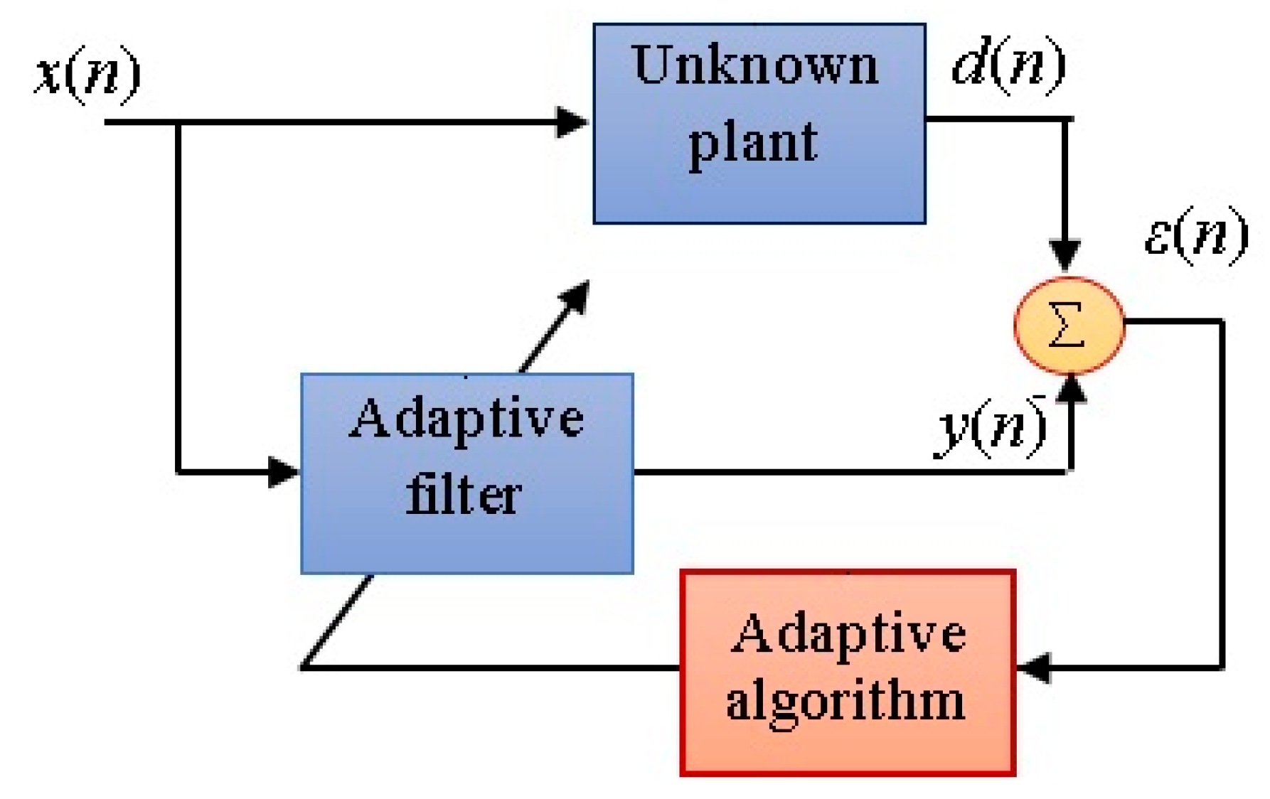
2.1. Preliminaries on Adaptive FIR and IIR Filtering

The FIR filter is shown in Figure 1 in the form of a single input transversal filter. The “adaptation” is that by which the weights are adjusted or adapted in response to a function of the error signal. When the weights are in the adaptation course, they are a function of the input samples and not just the output so that the transversal filter’s output is not characterized a linear in terms of the input.

$$y\left(n\right)={\displaystyle \sum }_{k=0}^{N-1}{w}_k\left(n\right) x\left(n-k\right)$$

(1)

where N is the filter order. In vector notation,

$$y\left(n\right)={\mathit{X}}_N^T\left(n\right) {\mathit{C}}_N\left(n\right)$$

(2)

and the error signal is given as

$$\epsilon \left(n\right)=d\left(n\right)-y\left(n\right)=d\left(n\right)-{\mathit{X}}_N^T\left(n\right) {\mathit{C}}_N\left(n\right)$$

(3)

where $d\left(n\right)$ is the desired signal, $y\left(n\right)$ is the filter output, ${\mathit{X}}_N^T\left(n\right)$ is the input signal vector, ${\mathit{X}}_N^T\left(n\right)=\left[x\left(n\right) x\left(n-1\right)\cdots x\left(n-N+1\right)\right]$, ${\mathit{C}}_N\left(n\right)=\left[C_o\left(n\right) C_1\left(n\right) \cdots C_{N-1}\left(n\right)\right]$ is the coefficient vector, n representing the time index, the superscript T denoting transpose operator, and the subscript N representing the dimension of a vector.

Remark 1: 

To a set of points of the inputs sequence $x\left(n\right)$ and the reference waveform $d\left(n\right)$ there corresponds an optimum coefficient vector or impulse response ${\mathit{C}}_N\left(n\right)$. Given another set of points, there is no guarantee that the resulting optimum vector is related to the first unless the properties of the waveform do not change over different sections. Based on this, we can formulate the following assumption.

Assumption (H1). 

The input sequence $x\left(n\right)$ and the reference waveform $d\left(n\right)$ are stochastic processes. Then the error $\epsilon \left(n\right)$ defined by (3) is also stochastic.

The performance function or the mean-square error $E_{ms}$ is defined as

$$E_{ms}=E\{{\left|\epsilon \left(n\right)\right|}^2\}$$

(4)

Then,

$$E_{ms}=E\{{\left|d\left(n\right)-y\left(n\right)\right|}^2\}$$

(5)

Expanding and using (2) we obtain,

$$E_{ms}=E\{{\left|d\left(n\right)\right|}^2\}-{\mathit{C}}_N^{T}Re\left[E\{d^{*}\left(n\right){\mathit{X}}_N\left(n\right)\}\right]+{\mathit{C}}_N^{T}E\{{\mathit{X}}_N\left(n\right){\mathit{X}}_N^{\prime }\left(n\right)\}{\mathit{C}}_N^{*}$$

(6)

where $\ast$ and ${}^{\prime }$ denote conjugate and conjugate transpose, respectively, and the time index n is omitted from ${\mathit{C}}_N$ for simplicity. If we define the expected value of $d\left(n\right)$ as

$$D_{ms}\stackrel{\Delta }{=}E\{{\left|d\left(n\right)\right|}^2\}$$

(7)

and the ensemble or statistical autocorrelation matrix ${\mathit{R}}_{ms}$ of $x\left(n\right)$ as

$${\mathit{R}}_{ms}\stackrel{\Delta }{=} E\{{\mathit{X}}_N\left(n\right){\mathit{X}}_N^{\prime }\left(n\right)\}$$

(8)

which is a Toeplitz matrix and the ensemble average cross-correlation vector as

$${\mathit{P}}_{ms}\stackrel{\Delta }{=} E\{d^{*}\left(n\right){\mathit{X}}_N\left(n\right)\}$$

(9)

Remark 2: 

The matrix ${\mathit{R}}_{ms}$ is designated as the “input correlation matrix”, while ${\mathit{P}}_{ms}$ is the cross-correlations between the desired response and the input components. The main diagonal terms of The matrix ${\mathit{R}}_{ms}$ are the mean squares of the input components, and the cross terms are the cross-correlations among the input components. The elements of ${\mathit{R}}_{ms}$ are all constant second-order statistics when ${\mathit{X}}_N\left(n\right)$ and are stationary.

Then, $E_{ms}$ can be written as

$$E_{ms}=D_{ms}-2{\mathit{C}}_N^{T}Re\{{\mathit{P}}_{ms}\}+{\mathit{C}}_N^T {\mathit{R}}_{ms}{\mathit{C}}_N^{*}$$

(10)

which shows that $E_{ms}$ has a quadratic form. To find the choice for C_N that minimizes $E_{ms}$, we find the gradient of $E_{ms}$ w.r.t. C_N and find the optimum value of the weights ${\mathit{C}}_{ms}^o$ which sets it to zero. This leads to,

$${\mathit{R}}_{ms}{\mathit{C}}_{ms}^o=Re\{{\mathit{P}}_{ms}\}$$

(11)

The solution is unique if ${\mathit{R}}_{ms}$ is invertible, and then

$${\mathit{C}}_{ms}^o=R_{ms}^{-1}Re\{{\mathit{P}}_{ms}\}$$

(12)

which is the Wiener–Hopf equation in matrix form. Recursive filters, like IIR, with poles as well as zeros would offer the same advantages (resonance, sharper cut off, etc.) that nonrecursive filters offer in time-invariant applications. The recursive filters have two main weakness points, they become unstable if the poles move outside the unit circle and their performance indices are generally nonquadratic and may even have a local minimum. The adaptive IIR filter may be represented in the standard adaptive model as illustrated in Figure 2.

The input–output relationship is expressed as

$$y\left(n\right)={\displaystyle \sum }_{k=0}^M{b}_{k}x\left(n-k\right)+{\displaystyle \sum }_{k=1}^L{a}_{k}y\left(n-k\right)$$

(13)

where $b_k$’s and $a_k$’s are the IIR filter coefficients, and $y\left(n\right)$ and $x\left(n\right)$ are the output and input of the IIR filter, respectively. The IIR filter is characterized by the following transfer function [1].

$$H\left(z\right)=\frac{Y\left(z\right)}{X\left(z\right)}=\frac{b_o+b_1{z}^{-1}+\cdots +b_M{z}^{-1}}{1-a_1{z}^{-1}+\cdots +a_L{z}^{-1}}=\frac{{\sum }_{k=0}^M{b}_k z^{-k}}{1-{\sum }_{k=1}^L{b}_k z^{-k}}$$

(14)

Note that in (13) the current output sample is a function of the past output $y\left(n-k\right)$, as well as the present and past input sample $x\left(n\right)$, and $x\left(n-k\right)$, respectively. The powerfulness of the IIR filter comes from the feedback connection it has where it provides an additional flexibility. Due to this, the IIR filter usually needs less parameters than the FIR filter for the same sets of specifications.

Newton’s and steepest descent methods are used for descending toward the minimum on the performance surface. Both require an estimation of the gradient in each iteration. The gradient estimation method is general because they are based on taking differences between estimated points on the performance surface, that is, the difference between estimates of the error $\mathit{\epsilon }\left(\mathit{n}\right)$. In this subsection, we will use another algorithm for descending on the performance surface, known as Least Mean Square (LMS) algorithm and will be investigated on both FIR and IIR digital filters.

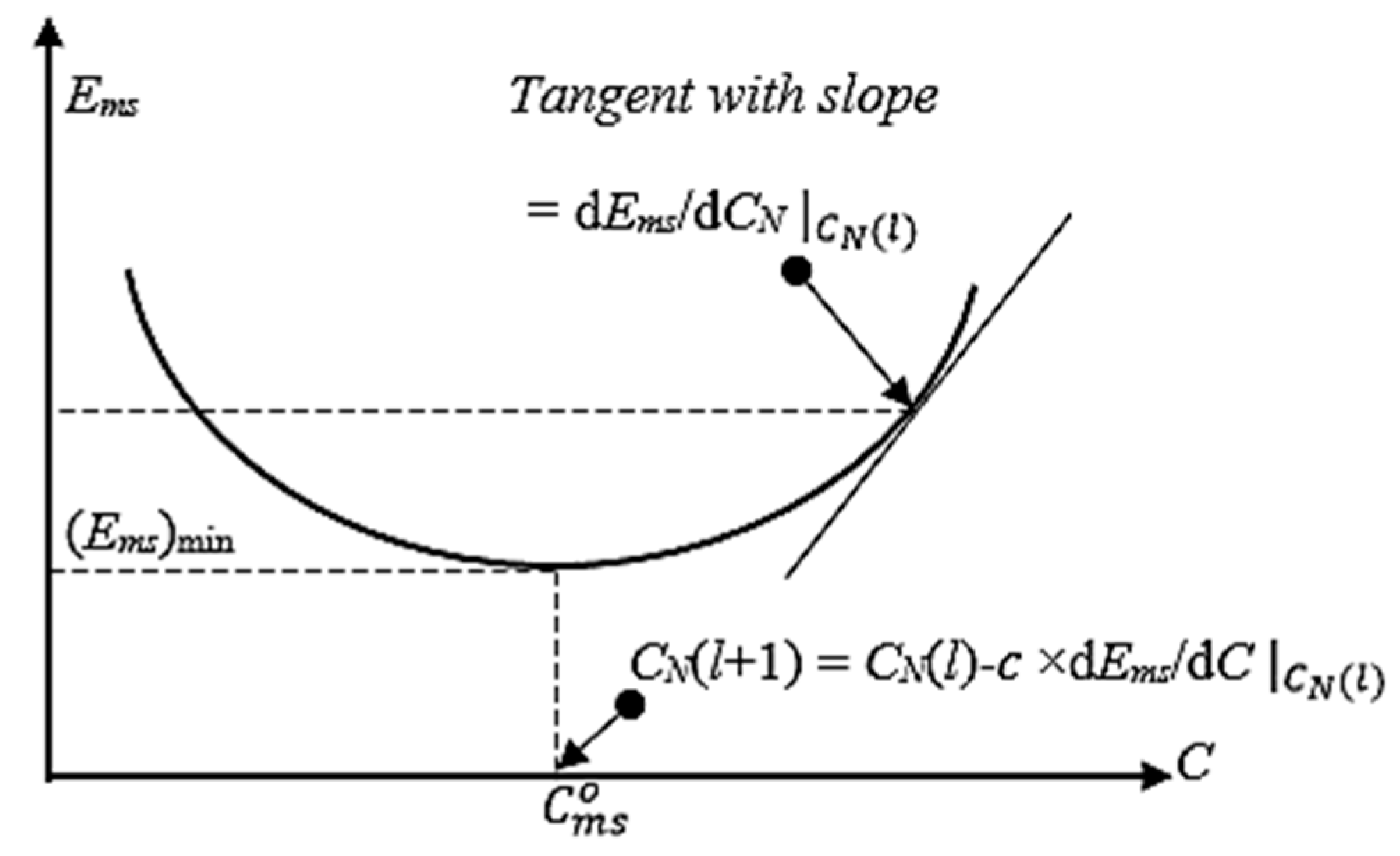
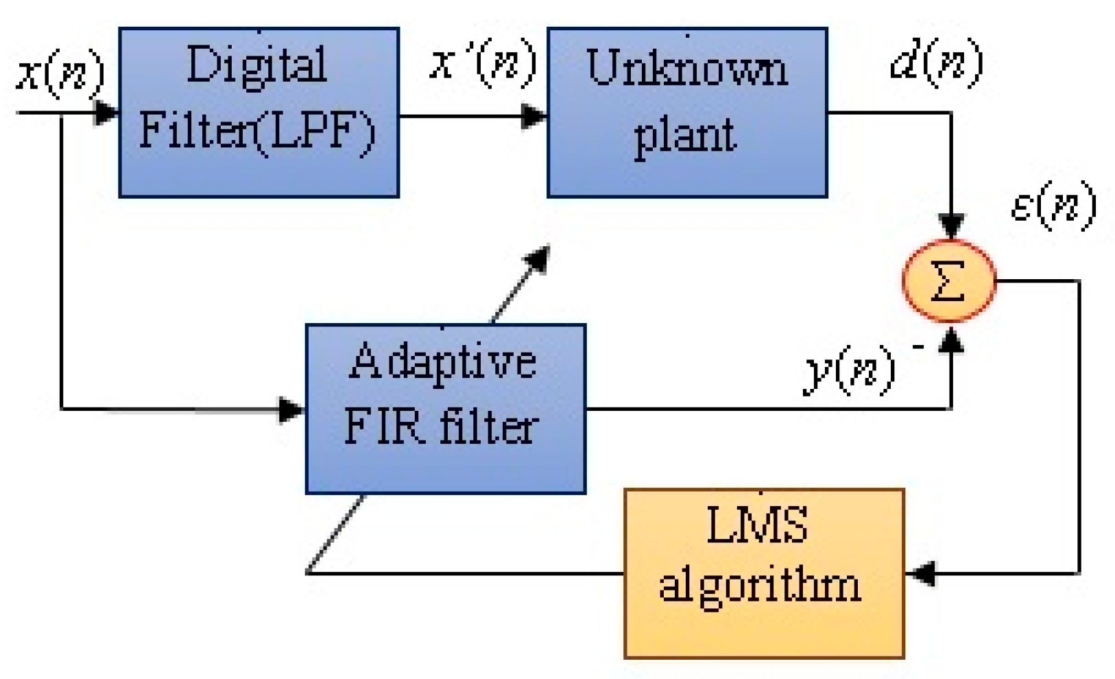
2.2. The LMS Algorithm and Adaptive FIR Filtering

Given a record of data ($x\left(n\right)$, $d\left(n\right)$), one can compute ${\mathit{R}}_{ms}$ and ${\mathit{P}}_{ms}$; ${\mathit{R}}_{ms}$ might not be invertible and, if it is, its inversion requires high numerical precision. A method depending on search techniques has the advantage of being simple to implement but at the expense of some inaccuracy in the final estimate. We use the gradient or steepest descent searching technique to find ${\mathit{C}}_{ms}^o$ iteratively. This technique is applicable to the minimization of the quadratic performance function $E_{ms}$, since it is a convex function of the coefficients C_N, i.e., it possesses a global minimum. A gradient vector is computed as $\partial E_{ms}/\partial {\mathit{C}}_N$, $i=1,\cdots ,N-1$, at this point each tap weight is changed in the direction opposite to its corresponding gradient component and by an amount proportional to the size of that component. Therefore

$${\mathit{C}}_N\left(l+1\right)={\mathit{C}}_N\left(l\right)-\mu {\nabla }_{C_N}{E}_{ms}$$

(15)

where ${\nabla }_C{E}_{ms}$ is the gradient vector, the subscript indicating that the gradient is taken w.r.t. to the components of the filter coefficients vector ${\mathit{C}}_N$, $l$ is the iteration number, and $\mu$ is the convergence factor that regulates the speed and the stability of the adaptation. It is clear from Figure 3 which represents the one-dimensional case, how repeating this procedure leads to the minimum of $E_{ms}$ and hence the optimal value ${\mathit{C}}_{ms}^o$. Approximating the gradient of $E_{ms}$ by the gradient of the instantaneous squared error, i.e.,

$${\nabla }_{C_N}{E}_{ms}={\nabla }_{C_N}E\{{\left|\epsilon \left(n\right)\right|}^2\}\approx {\nabla }_{C_N}{\left|\epsilon \left(n\right)\right|}^2=2\epsilon \left(n\right)·\frac{d\epsilon \left(n\right)}{d C_N}=2\epsilon \left(n\right){\mathit{X}}_N\left(n\right)$$

(16)

We may write ${\mathit{C}}_N\left(l+1\right)$ as

$${\mathit{C}}_N\left(l+1\right)={\mathit{C}}_N\left(l\right)-\mu {\nabla }_{C_N}{\left|\epsilon \left(n\right)\right|}^2={\mathit{C}}_N\left(l\right)+2\mu \epsilon \left(n\right) {\mathit{X}}_N\left(n\right)$$

(17)

Usually, ${\mathit{C}}_N\left(l\right)$ is updated for every sample as is the case when variations are to be tracked in an estimation process. When this is true, $l=n$. The LMS algorithm is summarized as follows

$$\{\begin{array}{c}\begin{array}{c}y\left(n\right)={\mathit{C}}^T\left(n-1\right){\mathit{X}}_N\left(n\right) \\ \epsilon \left(n\right)=d\left(n\right)-y\left(n\right) \\ {\mathit{C}}_N\left(n\right)={\mathit{C}}_N\left(n-1\right)+2\mu \epsilon \left(n\right){\mathit{X}}_N\left(n\right)\end{array}\end{array}$$

(18)

A flowchart for the LMS algorithm is given in Figure 4. A convergence analysis for the LMS algorithm has been done in [1] and concluded that to achieve convergence the value of $\mu$ is found as,

$$0<\mu <\frac{1}{{\lambda }_{max}}$$

(19)

where ${\lambda }_{max}$ is the maximum eigenvalue of ${\mathit{R}}_{ms}$.

2.3. Adaptation of IIR Digital Filter Based on LMS Algorithm

To develop an algorithm for the recursive IIR filter, let us define the time-varying vector ${\mathit{C}}_N\left(n\right)$ and the signal $U\left(n\right)$ as follows

$${\mathit{C}}_N\left(n\right)=\left[b_o\left(n\right) b_1\left(n\right)\cdots \cdots b_M\left(n\right) a_1\left(n\right)\cdots \cdots a_L\left(n\right)\right]$$

(20)

$$\mathit{U}\left(n\right)=\left[x\left(n\right) x\left(n-1\right)\cdots x\left(n-M\right) y\left(n-1\right)\cdots \cdots y\left(n-L\right)\right]$$

(21)

From Figure 2 and Equation (10), we can write

$$\epsilon \left(n\right)=d\left(n\right)-y\left(n\right)=d\left(n\right)-C_N{\left(n\right)}^{T}U\left(n\right)$$

(22)

This is quite similar to the nonrecursive case in (3). The main difference being that $\mathit{U}\left(n\right)$ contains values of $y\left(n\right)$ as well as $x\left(n\right)$. We again use the gradient approximation

$$\begin{array}{ll}{\nabla }_{C_N}{E}_{ms}={\nabla }_{C_N}E& \{{\left|\epsilon \left(n\right)\right|}^2\}\approx \frac{\partial {\epsilon }^2}{\partial {\mathit{C}}_N\left(n\right)}=2\epsilon \frac{\partial \epsilon }{\partial {\mathit{C}}_N\left(n\right)}\\ & =2\epsilon {\left[\frac{\partial \epsilon \left(n\right)}{\partial b_o\left(n\right)}\cdots \frac{\partial \epsilon \left(n\right)}{\partial b_M\left(n\right)}\frac{\partial \epsilon \left(n\right)}{\partial a_1\left(n\right)}\cdots \frac{\partial \epsilon \left(n\right)}{\partial a_L\left(n\right)}\right]}^T\\ & =-2\epsilon \left(n\right){\left[\frac{\partial y\left(n\right)}{\partial b_o\left(n\right)}\cdots \frac{\partial y\left(n\right)}{\partial b_M\left(n\right)}\frac{\partial y\left(n\right)}{\partial a_1\left(n\right)}\cdots \frac{\partial y\left(n\right)}{\partial a_L\left(n\right)}\right]}^T\end{array}$$

(23)

The derivatives in (23) present a special problem because $y\left(n\right)$ is now a recursive function. Using (13) we define

$$\begin{array}{c}{\alpha }_k\left(n\right)\stackrel{\Delta }{=}\frac{\partial y\left(n\right)}{\partial b_k\left(n\right)}=x\left(n-k\right)+{\sum }_{l=1}^L{a}_l\frac{\partial y\left(n-l\right)}{\partial b_k\left(n\right)}=x\left(n-k\right)+{\sum }_{l=1}^L{a}_l{\alpha }_k\left(n-l\right),\\ k=0,1,\cdots ,M\end{array}$$

(24)

$$\begin{array}{c}{\beta }_k\left(n\right) \stackrel{\Delta }{=}\frac{\partial y\left(n\right)}{\partial a_k\left(n\right)}=y\left(n-k\right)+{\sum }_{l=1}^L{a}_l\frac{\partial y\left(n-l\right)}{\partial a_k\left(n\right)}=y\left(n-k\right)+{\sum }_{l=1}^L{a}_l{\beta }_k\left(n-l\right), \\ k=1,\cdots ,L\end{array}$$

(25)

With the derivatives defined in this manner, we have

$${\nabla }_{C_N}{E}_{ms}=-2\epsilon \left(n\right){\left[{\alpha }_o\left(n\right)\cdots {\alpha }_M\left(n\right) {\beta }_1\left(n\right)\cdots {\beta }_L\left(n\right)\right]}^T$$

(26)

Now we write the LMS algorithm as follows

$${\mathit{C}}_N\left(n+1\right)=C_N\left(n\right)-\mu {\nabla }_C{E}_{ms}$$

(27)

With nonquadratic error surface, we now have a convergence parameter $\mu$ for both $a$ and $b$. We may even wish to have this factor vary with time. Using the current values of the $a$’s and in (24) and (25), the LMS algorithm computation for recursive adaptive IIR filter as follows

$$\{\begin{array}{c}y\left(n\right)={\mathit{C}}_N^T\left(n\right)\mathit{U}\left(n\right)\\ {\alpha }_k\left(n\right)=x\left(n-k\right)+{\displaystyle {\displaystyle \sum }_{l=1}^L}{a}_l{\alpha }_k\left(n-l\right) , 0\le k\le M \\ {\beta }_k\left(n\right)=y\left(n-k\right)+{\displaystyle {\displaystyle \sum }_{l=1}^L}{a}_l{\beta }_k\left(n-l\right) , 1\le k\le L\\ {\nabla }_C{E}_{ms}=-2\epsilon \left(n\right){\left[ {\alpha }_o\left(n\right)\cdots {\alpha }_M\left(n\right) {\beta }_1\left(n\right)\cdots {\beta }_L\left(n\right)\right]}^T\\ {\mathit{C}}_N\left(n+1\right)={\mathit{C}}_N\left(n\right)-\mu {\nabla }_{C_N}{E}_{ms}\end{array}$$

(28)

Initialization is the same as in the case adaptive FIR filter except that here, the $\alpha$’s and $\beta$’s should be set initially to zero unless their values are known.

3. Evolutionary Computation: The Genetic Algorithm (GA)

The GA is a global, parallel, robust stochastic search algorithm based on the principle of natural selection and natural genetic process that combines the notion of survival of the fittest, random search, and parallel evaluation of points in the search space. GAs start with the initial strings population (denoted chromosome), which map individuals (candidate solutions) to the optimization problem, and the individuals’ population develops into the better solutions using GA operators described next. Typically, the objective of GA is commonly stated as the maximization of fitness function $F\left(t\right)$ given by [31,32]

$$F\left(t\right)=\frac{1}{1+f\left(t\right)}$$

(29)

where $f\left(t\right)$ is the cost function to be minimized. In adaptive filtering, GA operates on a set of filter parameters (the population of the chromosomes), in which a fitness values are specified to each individual chromosome. The cost function $f\left(t\right)$ in adaptive filtering is taken as the Mean Square Error (MSE) ${\epsilon }_j{}^2$, which is given by

$$f\left(t\right)={\epsilon }_j{}^2=\frac{1}{t_e}{\displaystyle \sum }_{i=1}^{te}{\left[d\left(n\right)-y_j\left(n\right)\right]}^2$$

(30)

where $t_e$ is the size of the window over which the errors will be added and stored, $y_j\left(n\right)$ is the estimated output associated with the j-th set of estimated filter coefficients, and j is the chromosome index.

GA consists of key three stages: (1) selection, (2) cross-over, and (3) mutation. The Selection denotes the procedure of selecting a group of chromosomes from the population that will subsidize to the formation of the offspring for the subsequent generations. The chromosomes having greater fitness values in the population will get a higher probability of being selected for the following generation. Numerous techniques have been proposed for the selection process; for example, see [32]. The evolutionary process usually starts from a randomly generated population; in each generation, the fitness of each individual in the population is evaluated, which is determined by a problem specific fitness function of (30). Then, multiple individuals are randomly selected from the current population based on their fitness, and combined by cross-over operation and/or undergo mutation operation. The mutation operator is another technique of the GA to explore the cost surface, and it can create chromosomes that never occurs in the early populations and maintain the GA from approaching the solution quickly before examining the entire cost error surface [33,34]. The new offsprings (the set of filter coefficients) then form the basis of the next generation. The basic cycle of GA is depicted in Figure 5.

Also, the GA will search within each generation for the minimum of the estimation error ${\epsilon }_{min}=\min ({\epsilon }_j{}^2)$ for every chromosome in the entire population with an attempt of driving ${\epsilon }_{min}$ to an acceptable minimum value or to zero in the subsequent generations. Adopting the standard GA itself in adaptive filtering leads to a slow convergence rate, this is due to the tremendously big searching space of the GA, which makes the mutation (randomization) process wasting time in examining solutions over improper directions.

4. Proposed Adaptive System Identification for FIR and IIR Digital Filters

In this section, the main results of this work will be presented and analyzed with both white and colored signals. The effect of colored input signals on the adaptation process is discussed first followed by the proposed LMS-GA learning tool.

4.1. The Effect of Colored Signal On the Adaptation Process of LMS Algorithm

Suppose that the input signal $x\left(n\right)$ is passed through a digital Low-Pass Filter (LPF), and then the output of the digital filter is applied to the adaptive system as shown in Figure 6. To show the effect of the digital low-pass filter on the adaptation process, let us discuss the difference between the input and the output signals of the digital filter. The input to the digital filter is shown in Figure 7a, where Figure 7b shows the autocorrelation ${\varphi }_{ij} \left(t, n\right)$, where ${\varphi }_{ij} \left(t, n\right)=x_i x_j$, with $x_i$ and $x_j$ are samples of x(n), $i,j=1,2,\cdots \mathrm{are} \mathrm{the} \mathrm{time} \mathrm{indices} \mathrm{of} x\left(n\right)$, and $t=\left|i-j\right|$. We notice from Figure 7 that the input signal $x\left(n\right)$ is an impulse signal at each instant and is correlated with itself only and it is never correlated with other impulses. The output of the digital low-pass filter is also a random signal as shown in Figure 8.

The spectral characteristics of the random signal are obtained by calculating the Fourier-transform for the correlation ${\varphi }_{ij} \left(t, n\right)$ of the input signal $x\left(n\right)$. The power spectral density of the input signal $x\left(n\right)$ is shown in Figure 9, which is flat for all frequencies (White spectrum).

It is seen from the demonstration of the LMS convergence that the algorithm convergence time $\tau$ is determined as

$$\tau =\frac{1}{\mu {\lambda }_{min}}=\frac{1}{2\alpha }\frac{{\lambda }_{max}}{{\lambda }_{min}}$$

(31)

where $\alpha =\mu \frac{{\lambda }_{max}}{2}$, ${\lambda }_{max}$, and ${\lambda }_{min}$ are the minimum and maximum eigenvalues of the autocorrelation matrix ${\mathit{R}}_{ms}$ respectively. The ratio of the maximum to the minimum eigenvalue is called the eigenvalue disparity and determines the speed of convergence. The convergence time depends only on the nature of the input sequence x(n) and not on the desired signal d(n). The matrix ${\mathit{R}}_{ms}$ is given as

$${\mathit{R}}_{ms}=\left[\begin{array}{ccccc}{\varphi }_{00}(0,n)& {\varphi }_{01}(1,n)& {\varphi }_{02}(2,n)& \cdots & {\varphi }_{0 }{}_{N-1}(N-1,n)\\ {\varphi }_{10}(1,n)& {\varphi }_{11}(0,n)& {\varphi }_{12}(1,n)& \cdots & {\varphi }_{1 }{}_{N-1}(N-2,n)\\ {\varphi }_{20}(2,n)& {\varphi }_{21}(1,n)& {\varphi }_{22}(0,n)& \cdots & {\varphi }_{2 }{}_{N-1}(N-3,n)\\ ⋮& ⋮& ⋮& ⋮& ⋮\\ {\varphi }_{N-1 0}(N-1,n)& {\varphi }_{N-1 1}(N-2,n)& {\varphi }_{N-1 2}(N-3,n)& \cdots & {\varphi }_{N-1 N-1}(0,n)\end{array}\right]$$

(32)

where ${\varphi }_{ij} \left(t, n\right)= x_i\left(n\right) x_j\left(n\right)$, with $i,j=1,2,\cdots ,N-1$, $t=\left|i-j\right|$. It is seen from (31) that the convergence time is inversely proportional to $\mu$ and depends only on the nature of the input sequence $x\left(n\right)$. The physical interpretation of the eigenvalues ${\lambda }_i$ of ${\mathit{R}}_{ms}$ can be illustrated by comparing them with the spectrum of the input signal $x\left(n\right)$. It is a classical result of Toeplitz form theory that the eigenvalues are bounded by

$$X{\left(e^{j\omega }\right)}_{min}<{\lambda }_i<X{\left(e^{j\omega }\right)}_{max} , i=0,1,\dots , N-1$$

(33)

where $X\left(e^{j\omega }\right)$ is the power spectral density of the input or the Fourier-transform of the autocorrelation function ${\varphi }_{ij} \left(t, n\right)$ (elements of the ${\mathit{R}}_{ms}$ matrix). As the order of the matrix, N, tends to infinity:

$$\{\begin{array}{c}{\lambda }_{min}\to X{\left(e^{j\omega }\right)}_{min}\\ {\lambda }_{max}\to X{\left(e^{j\omega }\right)}_{max}\end{array}$$

(34)

Given that the convergence time $\tau$ can be expressed as in (31), we infer that the spectra that with the ratio of the maximum to minimum spectrum is large results in sluggish convergence. Spectra with an eigenvalue disparity near unity (i.e., flat spectra) lead to rapid convergence. The conjecture about such results is that large correlation among the input samples is related to a large eigenvalue disparity, which in turn decelerates the convergence of the adaptation process of the FIR filter.

Now, we show the effect of the colored signal $x^{\prime }\left(n\right)$ on the convergence speed of the adaptation process. The autocorrelation function ${{\varphi }^{\prime }}_{ij} \left(t, n\right)$ of the colored signal $x^{\prime }\left(n\right)$ is shown in Figure 10.

From Figure 10, we can verify that the impulse $x^{\prime }\left(0\right)$ is more correlated with itself and less with other impulses. The spectral density of the input signal can be obtained by computing the Fourier-transform of the autocorrelation function (the elements of ${\mathit{R}}_{ms}$ matrix) as shown in Figure 11. So that the eigenvalue disparity ${\lambda }_{max}/{\lambda }_{min}\to X{\left(e^{j\omega }\right)}_{max}/X{\left(e^{j\omega }\right)}_{min}$ will be larger than the white signal. Therefore, the effect of the colored signal will result in slow convergence.

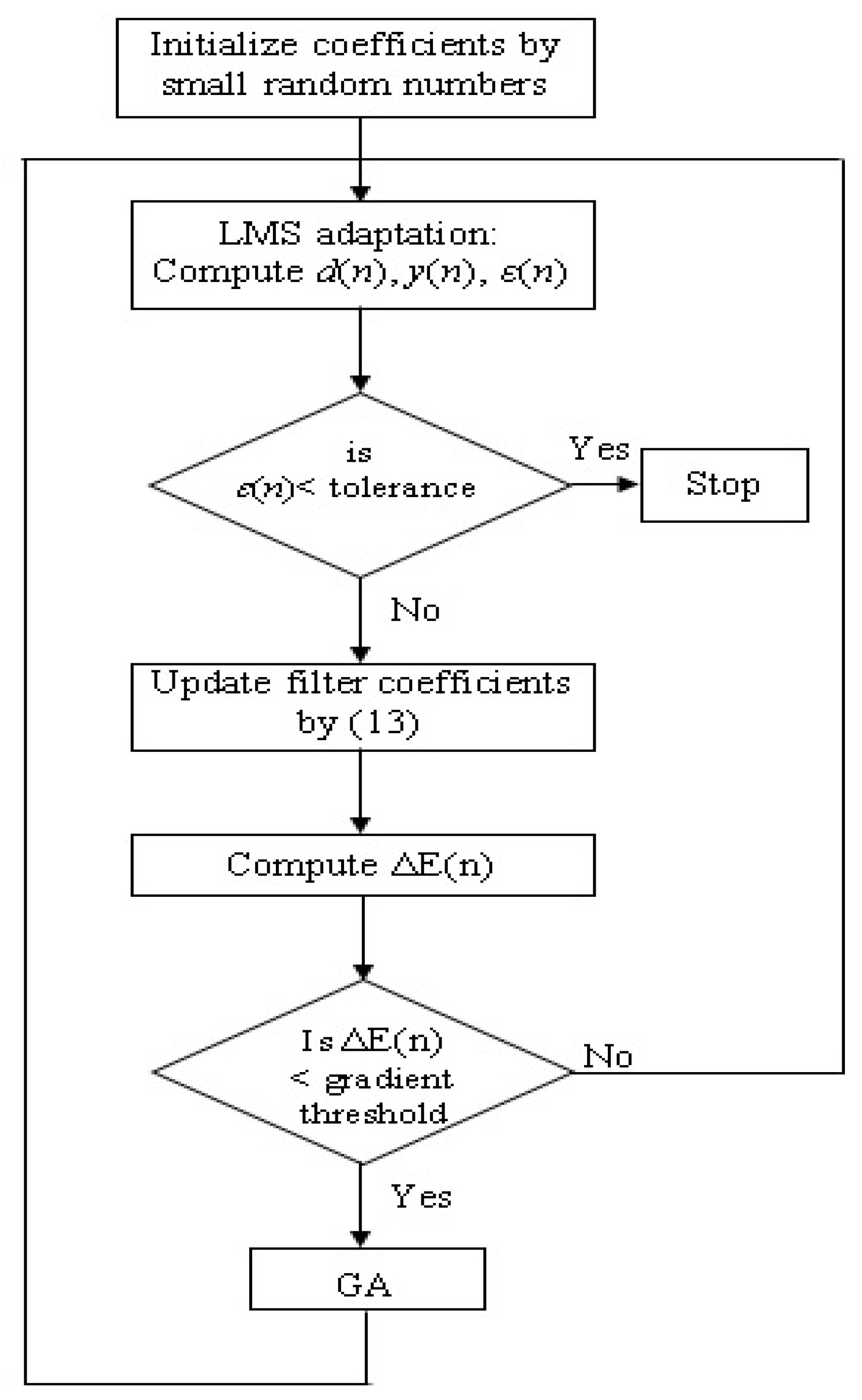
4.2. The Integrated LMS Algorithm with Genetic Search Approach (LMS-GA)

As said earlier, GA is slow for tuning in adaptive filtering; while, the gradient descent techniques behave well in local regions only. To overcome the difficulties of the GA and gradient descent methods, we propose in this section a novel approach for the learning the adaptive FIR and IIR filters that incorporates the quintessence and features of both algorithms.

The essential principle of our novel learning algorithm is to combine the evolutionary idea of GA into the gradient descent technique to give an organized random searching amid the gradient descent calculations. The filter coefficients are represented as a chromosome with a list of real numbers in our proposed technique. The LMS algorithm is embedded in the mutation process of GA to discover the fastest shortcut path in adjusting the optimal solution through the learning process. Each time the LMS learning tool get caught in a local minimum, or the convergence of the LMS algorithm is slow (i.e., the gradient of the error is within a specific range), we begin the GA by arbitrarily varying the estimated filter parameters values to obtain a new set of filter coefficients. The proposed learning algorithm, namely, LMS-GA, chooses the filter among the new filters and the first one with the smallest MSE (best fitness value) as the new candidate to the next evolution. The above process will be done more and more if the convergence speed is detected to be sluggish at uniform intervals or the LMS algorithm stuck in one more local minimum. In the suggested learning technique, the parameters of the filter are varied during each evolution according to

$${\mathrm{\Theta }}_i=\mathrm{\Theta }+{\sigma }_i \mathcal{D} 1\le i\le m$$

(35)

where $\mathcal{D}$ is the permissible offset range for each evolution, m is the offsprings number produced in the evolutions, ${\mathrm{\Theta }}_i$ denotes the i-th offsprings that are produced by the parents filter $\mathrm{\Theta }$, and ${\sigma }_i\in$ [−1, +1] is a random number. To pick the optimum filter to be the next candidate amongst the sets of new offsprings in the course of each evolution, we calculate the MSE for each new filter (${\mathrm{\Theta }}_i$, $1\le i\le m$) by (30) for a block of time $t_e$. The filter with the smallest MSE will be selected as the next candidate for the subsequent phase of the learning process. We represent the behavior of the new proposed LMS-GA by the flowchart shown in Figure 12. The ΔE(n) in the flowchart of Figure 12 is the error gradient and defined as

$$\Delta E\left(n\right)=\frac{e\left(n\right)-e\left(n-\gamma \right)}{\gamma }$$

(36)

where $\gamma$ is the window size for estimation of $\Delta E$. The computational complexity of the LMS algorithm of the FIR filter for the case of the white input signal is found to be (2$N)$ multiplication per iteration, where $N$ is the length of the FIR filter. While the computational complexity required for the IIR filter is equal to $\left(M+L\right)\left(L+2\right)$, where $L$ is the backward length and $M$ is the forward length of the IIR filter for the same order of both FIR and IIR filters (i.e., $N=L+M$). The computational complexity of the LMS algorithm of the FIR filter with colored input signal is given as $N·P+2N$, where $P$ is the length of the digital LPF.

5. Numerical Results and Simulations

Consider the 4-Tap adaptive FIR filter in channel equalization application as a plant model for system identification:

$$H\left(z\right)=0.03+0.24z^{-1}+0.54z^{-2}+0.8z^{-3}$$

(37)

The basic idea of the system identification using adaptive FIR filtering depends on matching the coefficients of the adaptive filter to that of the plant. The convergence factor $\mu$ regulates the adaptation stability and convergence speed. A special class of input signal is generated to train the weights of the adaptive FIR filter, it consists of four level values (−3, −1, +1, and +3) and governed by a uniformly generated random input $R\in \left[0, 1\right]$ as shown in Figure 13, e.g., if the random number is $R_{oo}$, i.e., it is in the range [0, 0.25], then $x\left(n\right)=-3$, the same for other values of $R$.

These four level input values generated using the scheme proposed in Figure 13 are entered repeatedly into the input channel $x\left(n\right)$ of Figure 14 until a convergence is reached or a maximum number of iterations are achieved. The results of applying the standard LMS algorithm on an adaptive FIR filter to identify the parameters of (37) with different values of $\mu$ are shown in

Table 1. Simulation results of FIR adaptation (white signal).

Step Size µ	No. of Iterations	MSE/dB	Adaptive Filter Coefficients
			C1	C2	C3	C4
0.04	399	−167.200	0.03	0.24	0.54	0.8
0.045	130	−166.250	0.03	0.24	0.54	0.8
0.095	1911	−166.278	0.03	0.24	0.54	0.8

. The learning curves for three different values of $\mu$ are shown in Figure 15.

From the above results, we observe that the optimum value of $\mu$ that corresponds to fewer iterations is found to be (0.045). For the case of the colored input signal, the same input produced using the scheme of Figure 13 is applied on the input channel of Figure 6, we conclude that the spectra with the ratio of the maximum to minimum spectrum is large results in sluggish convergence. Spectra with an eigenvalue disparity near unity (i.e., flat spectra) lead to rapid convergence. The digital filter of Figure 6 used in this simulation is of 8-Tap FIR LPF type given as

$$\mathit{h}\left(\mathit{n}\right)=\left[\mathbf{0.0012654}-\mathbf{0.0052341}-\mathbf{0.0019735}-\mathbf{0.0023009} \mathbf{0.022366} \mathbf{0.12833} \mathbf{0.0013} \mathbf{0.0012}\right]$$

The plant dynamics is given in (37). Different $\mu$s have been used in colored input signal case study with the results given in

Table 2. Simulation results of the FIR adaptation (colored signal).

Step Size µ	No. of Iterations	MSE/dB	Adaptive Filter Coefficients
			C1	C2	C3	C4
0.9	2320	−135.591	0.03	0.24	0.54	0.8
3	358	−163.131	0.03	0.24	0.54	0.8
4	362	−173.604	0.03	0.24	0.54	0.8

. We note that the optimum value of $\mu$ that corresponds to the less number of iterations is found to be 3. The learning curves for different values of $\mu$ are illustrated in Figure 16. The best value of $\mu$ is found with MSE of -163.131 dB.

Concerning the adaptive IIR filter, the error surface is generally a multimodal against filter parameters. The adaptation techniques for the case of adaptive IIR filter can easily get stuck at a local minimum and escape away from the global minimum. Some of the adaptive IIR filter coefficients will be matched with that of the plant, and the other will be constant at specific values, which means that these coefficients are stuck at local minima. The following 1st order transfer function $H\left(z\right)$ is used to represent the plant

$$H\left(z\right)=\frac{0.6}{1-0.2z^{-1}}$$

(38)

The results of the system identification using IIR adaptive filtering are shown in

Table 3. Simulation of adaptive IIR filter (white signal).

Step Size µ	No. of Iterations	MSE/dB	Adaptive Filter Coefficients
			a	b
0.04	142	−157.373	−0.2	0.6
0.06	63	−143.939	−0.2	0.6
0.1	134	−174.030	−0.2	0.6

. As can be seen, the best value of $\mu$ was found to be 0.065. The IIR error surface here is a special case as it is an unimodal (local minimum does not exist) and having a global optimum only. However, the practical problem still exists here which is the pole of the adaptive filter may move outside of the unit circle resulting in an unstable system. To solve this problem, we use a certain criterion that states when the magnitude of the pole exceeds unity; we limit its magnitude to be less than one. The learning curves for different values of $\mu$ are shown in Figure 17.

The new LMS-GA learning tool can be applied to the system identification as shown in Figure 14 with FIR adaptive filter instead of an IIR one. Then, we can deduce the learning curve with window size 8 and offsprings m =5 and offset D = 0.02 as shown in Figure 18 and the comparison results with the standard LMS algorithm are listed in

Table 4. Simulation results of both standard LMS and LMS-GA algorithms for the FIR filter.

		Standard LMS Algorithm with Optimum µ	LMS-GA with Optimum µ
No. of Iterations		130	336
MSE (dB)		−166.250	−173.604
Filter Coefficients	C1	0.03	0.03
	C2	0.24	0.24
	C3	0.54	0.54
	C4	0.8	0.8

. One can see that the simple LMS algorithm is faster than the new learning algorithm because the LMS-GA is a random technique which is applied to a multimodal error surface. In the case of unimodal error surface (as the case of FIR adaptive filter), the simple LMS algorithm is a better choice than other algorithms like the LMS-GA learning tool.

The proposed LMS-GA learning tool is exploited to learn an adaptive IIR filter to recover the performance of the gradient descent technique (e.g., the LMS algorithm) with multimodal error surface. To compare the new LMS-GA learning tool with the standard LMS algorithm, we must determine the window size δ the window for estimation of ∆E and the Gradient Threshold (GT). These can be calculated from the learning curve of the simple LMS algorithm as follows, window size τ is calculated as being the number of iterations between the first iteration and the iteration at which the learning curve fluctuate with small variations. GT is calculated by determining the maximum and minimum values of these fluctuations. Now, GT can be determined as GT = (max.swing − min.swing)/δ. If these two parameters are calculated, we can apply the procedure of the new learning algorithm of Figure 12 on an adaptive IIR filter of a unimodal error surface as in (39). We conclude that the new learning algorithm will converge to the same MSE (the same MSE the pure LMS reached to it) but with a fewer number of iterations as shown in Figure 19.

6. Conclusions

In this work, adaptive algorithms are utilized to learn the parameters of the digital FIR and IIR filters such that the error signal is minimized. These algorithms are the standard LMS algorithm and the LMS-GA one. The numerical instabilities inherent in other adaptive techniques do not exist in the conventional LMS algorithm. Moreover, prior information of the signal statistics is not required, i.e., the autocorrelation and cross-correlation matrices. The LMS algorithm produces only estimated adaptive filter coefficients. These estimated coefficients match that of the plant progressively through time as the parameters are changed and the adaptive filter learns the signal characteristics, and then identifies the underlying plant. Due to the multimodality of the error surface of adaptive IIR filters, a new learning algorithm, namely, LMS-GA, is proposed in this paper, which integrates the genetic searching methodology LMS algorithm and speeds up the adaptation procedure and offers universal searching ability. Besides, the LMS-GA preserved the characteristics and the simplicity of the standard LMS learning algorithm, and it entailed comparatively fewer computations and had a fast convergence rate as compared to the standard GA. It is evident that the numerical simulations elucidated that the LMS-GA outperforms the standard LMS in terms of the capability to determine the global optimum solution and the faster convergence rate to this solution. Future work includes investigating the stability of the proposed algorithm as well as the validation of this algorithm with more realistic applications such as echo and noise cancelation. Investigating the performance of the proposed LMS-GA algorithm with that of the Prediction Error Method (PEM) is a good point for future study. Finally, the hardware complexity is very high in case of adaptive algorithms like LMS one, especially for higher accuracy and floating point calculations, this adds more overhead. So, future work might be to design a systolic array architecture to reduce this overhead.

References

1. Widrow, B.; Stearns, S.D. Adaptive Signal Processing; Prentice-Hall: Upper Saddle River, NJ, USA, 1985. [Google Scholar]
2. Avalos, J.G.; Sanchez, J.C.; Velazquez, J. Applications of Adaptive Filtering. In Adaptive Filtering Applications; InTech: London, UK, 2011; pp. 1–20. ISBN 978-953-307-306-4. [Google Scholar]
3. Raitio, T.; Suni, A.; Yamagishi, J.; Pulakka, H.; Nurminen, J.; Vainio, M.; Alku, P. HMM-Based Speech Synthesis Utilizing Glottal Inverse Filtering. IEEE Trans. Audio Speech Lang. Process. 2011, 19, 153–165. [Google Scholar] [CrossRef]
4. Karaboga, N.; Latifoglu, F. Elimination of noise on transcranial Doppler signal using IIR filters designed with artificial bee colony—ABC-algorithm. Digit. Signal Process. 2013, 23, 1051–1058. [Google Scholar] [CrossRef]
5. Khodabandehlou, H.; Fadali, M.S. Nonlinear System Identification using Neural Networks and Trajectory-Based Optimization. arXiv 2018, arXiv:1804.10346. [Google Scholar]
6. Zhang, W. System Identification Based on a Generalized ADALINE Neural Network. In Proceedings of the American Control Conference (ACC), New York, NY, USA, 11–13 July 2007; Volume 11, pp. 4792–4797. [Google Scholar]
7. Jaeger, H. Adaptive nonlinear system identification with echo state networks. In Proceedings of the Advances in Neural Information Processing Systems; MIT Press: Cambridge, MA, USA, 2003; pp. 593–600. [Google Scholar]
8. Subudhi, B.; Jena, D. A differential evolution based neural network approach to nonlinear system identification. Appl. Soft Comput. J. 2011, 11, 861–871. [Google Scholar] [CrossRef]
9. Ibraheem, K.I. System Identification of Thermal Process using Elman Neural Networks with No Prior Knowledge of System Dynamics. Int. J. Comput. Appl. 2017, 161, 38–46. [Google Scholar]
10. Panda, G.; Mohan, P.; Majhi, B. Expert Systems with Applications IIR system identification using cat swarm optimization. Expert Syst. Appl. 2011, 38, 12671–12683. [Google Scholar] [CrossRef]
11. Sarangi, A.; Sarangi, S.K.; Mukherjee, M.; Panigrahi, S.P. System identification by Crazy-cat swarm optimization. In Proceedings of the 2015 International Conference on Microwave, Optical and Communication Engineering (ICMOCE), Bhubaneswar, India, 18–20 December 2015; pp. 439–442. [Google Scholar]
12. Jiang, S.; Wang, Y.; Ji, Z. A new design method for adaptive IIR system identification using hybrid particle swarm optimization and gravitational search algorithm. Nonlinear Dyn. 2014, 79, 2553–2576. [Google Scholar] [CrossRef]
13. Widrow, B.; Kamenetsky, M. On the statistical efficiency of the LMS family of adaptive algorithms. IEEE Trans. Inf. Theory 1984, 30, 211–221. [Google Scholar] [CrossRef]
14. Widrow, B.; Mccool, J.; Ball, M. The Complex LMS Algorithm. Proc. IEEE 1974, 63, 719–720. [Google Scholar] [CrossRef]
15. Ghauri, S.A.; Sohail, M.F. System identification using LMS, NLMS and RLS. In Proceedings of the 2013 IEEE Student Conference on Research and Development (SCOReD), Putrajaya, Malaysia, 16–17 December 2013; pp. 65–69. [Google Scholar]
16. Chen, W.; Nemoto, T.; Kobayashi, T.; Saito, T.; Kasuya, E.; Honda, Y. ECG and heart rate detection of prenatal cattle foetus using adaptive digital filtering. In Proceedings of the 22nd Annual International Conference of the IEEE Engineering in Medicine and Biology Society, Chicago, IL, USA, 23–28 July 2000; pp. 962–965. [Google Scholar]
17. Ma, G.; Gran, F.; Jacobsen, F.; Agerkvist, F.T. Adaptive feedback cancellation with band-limited LPC vocoder in digital hearing aids. IEEE Trans. Audio Speech Lang. Process. 2011, 19, 677–687. [Google Scholar]
18. Pereira, R.R.; Silva, C.H.d.; Silva, L.E.B.d.; Lambert-Torres, G. Application of Adaptive Filters in Active Power Filters. In Proceedings of the Brazilian Power Electronics Conference, Bonito-Mato Grosso do Sul, Brazil, 27 September–1 October 2009; Volume 1, p. 264. [Google Scholar]
19. Su, F.H.; Tu, Y.Q.; Zhang, H.T.; Xu, H.; Shen, T.A. Multiple Adaptive Notch Filters Based A Time-varying Frequency Tracking Method for Coriolis Mass Flowmeter. In Proceedings of the World Congress on Intelligent Control and Automation (WCICA), Jinan, China, 7–9 July 2010; pp. 6782–6786. [Google Scholar]
20. Neubauer, A. Non-Linear Adaptive Filters Based on Genetic Algorithms with Applications to Digital Signal Processing. In Proceedings of the 1995 IEEE International Conference on Evolutionary Computation, Perth, WA, Australia, 29 November–1 December 1995; pp. 3–8. [Google Scholar]
21. Nowaková, J.; Pokorný, M. System Identification Using Genetic Algorithms. In Proceedings of the Fifth International Conference on Innovations in Bio-Inspired Computing and Applications IBICA, Ostrava, Czech Republic, 23–25 June 2014. [Google Scholar]
22. Xia, W.; Wang, Y. A variable step-size diffusion LMS algorithm over networks with noisy links. Signal Process. 2018, 148, 205–213. [Google Scholar] [CrossRef]
23. Niu, Q.; Chen, T. A New Variable Step Size LMS Adaptive Filtering Algorithm. In Proceedings of the Chinese Control and Decision Conference (CCDC), Shenyang, China, 9–11 June 2018; pp. 1–4. [Google Scholar]
24. Yang, Q.; Lee, K.; Kim, B. Development of Multi-Staged Adaptive Filtering Algorithm for Periodic Structure-Based Active Vibration Control System. Appl. Sci. 2019, 9, 611. [Google Scholar] [CrossRef]
25. Huang, W.; Li, L.; Li, Q.; Yao, X. Diffusion robust variable step-size LMS algorithm over distributed networks. IEEE Access 2018, 6, 47511–47520. [Google Scholar] [CrossRef]
26. Bershad, N.J.; Eweda, E.; Bermudez, J.C.M. Stochastic analysis of the LMS algorithm for cyclostationary colored Gaussian and non-Gaussian inputs. Digit. Signal Process. 2019, 88, 149–159. [Google Scholar] [CrossRef]
27. Zhang, S.; Wang, Y.S.; Guo, H.; Yang, C.; Wang, X.L.; Liu, N.N. A normalized frequency-domain block filtered-x LMS algorithm for active vehicle interior noise control. Mech. Syst. Signal Process. 2019, 120, 150–165. [Google Scholar] [CrossRef]
28. Zenere, A.; Zorzi, M. On the coupling of model predictive control and robust Kalman filtering. IET Control Theory Appl. 2018, 12, 1873–1881. [Google Scholar] [CrossRef]
29. Zenere, A.; Zorzi, M. Model Predictive Control meets robust Kalman filtering. IFAC-PapersOnLine 2017, 50, 3774–3779. [Google Scholar] [CrossRef]
30. Zorzi, M.; Sepulchre, R. AR Identification of Latent-Variable Graphical Models. IEEE Trans. Automat. Contr. 2016, 61, 2327–2340. [Google Scholar] [CrossRef]
31. Ibraheem, K.I.; Alyaa, A.A. Application of an Evolutionary Optimization Technique to Routing in Mobile Wireless Networks. Int. J. Comput. Appl. 2014, 99, 24–31. [Google Scholar]
32. Ibraheem, I.K.; Alyaa, A.A. Design of a Double-objective QoS Routing in Dynamic Wireless Networks using Evolutionary Adaptive Genetic Algorithm. Int. J. Adv. Res. Comput. Commun. Eng. 2015, 4, 156–165. [Google Scholar]
33. Lu, T.; Zhu, J. Genetic Algorithm for Energy-Efficient QoS Multicast Routing. IEEE Commun. Lett. 2013, 17, 31–34. [Google Scholar] [CrossRef]
34. Ahn, C.W.; Ramakrishna, R.S. A Genetic Algorithm for Shortest Path Routing Problem and the Sizing of Populations. IEEE Trans. Evol. Comput. 2002, 6, 566–579. [Google Scholar]
Figure 1. Adaptive finite impulse response (FIR) filter implemented as transversal filter [1].
Information 10 00176 g001
Figure 2. Recursive adaptive infinite impulse response (IIR).
Information 10 00176 g002
Figure 3. Gradient descent on a one-dimensional projection of a quadratic performance function.
Information 10 00176 g003
Figure 4. Flowchart of the least mean squares (LMS) algorithm.
Information 10 00176 g004
Figure 5. GA three steps: Selection, cross-over, and mutation are involved in creating the evolution from one generation to the next.
Information 10 00176 g005
Figure 6. System identification configuration for the case of the colored input signal.
Information 10 00176 g006
Figure 7. The input signal and its autocorrelation: (a) the input signal x ( n ) to the digital LPF and (b) the autocorrelation ϕ i j   ( t ,   n ) of the input signal x ( n ) with i = j , where   ϕ i j   ( t ,   n ) =   x i ( n )   x j ( n ) ,   with   i , j = 1 , 2 , , N 1 ,   t = | i j | .
Information 10 00176 g007
Figure 8. The output of the digital low-pass filter.
Information 10 00176 g008
Figure 9. The power spectral density of the input signal x(n).
Information 10 00176 g009
Figure 10. The autocorrelation of the colored signal x ( n ) .
Information 10 00176 g010
Figure 11. The power spectral density of the digital filter output x ( n ) .
Information 10 00176 g011
Figure 12. Flowchart of the new learning algorithm (LMS-GA).
Information 10 00176 g012
Figure 13. Four levels input scheme used to train FIR and IIR adaptive filters.
Information 10 00176 g013
Figure 14. System identification block diagram.
Information 10 00176 g014
Figure 15. The learning curves for FIR adaptive filter with LMS algorithm: (a) μ = 0.045 , (b) μ = 0.04 , and (c) μ = 0.095 .
Information 10 00176 g015
Figure 16. The learning curves for the case of the colored input signal, (a) μ = 3 , (b) μ = 0.9 , and (c) μ = 4 .
Information 10 00176 g016
Figure 17. The learning curves for the case of IIR adaptive filter, (a) μ = 0.06 , (b) μ = 0.04 , and (c) μ = 0.1 .
Information 10 00176 g017
Figure 18. The learning curve of the FIR adaptive filter with integrated LMS-GA.
Information 10 00176 g018
Figure 19. The convergence performance of the LMS-GA tool for adaptive IIR filter.
Information 10 00176 g019