
Emission Abatement Technology Selection, Routing and Speed Optimization of Hybrid Ships


1
Department of Mechanical Engineering, Aalto University, Otakaari 4, 02150 Espoo, Finland
2
School of Technology and Innovations, University of Vaasa, Wolffintie 34, 65200 Vaasa, Finland
*
Author to whom correspondence should be addressed.
J. Mar. Sci. Eng. 2021, 9(9), 944; https://doi.org/10.3390/jmse9090944
Submission received: 8 August 2021
/
Revised: 24 August 2021
/
Accepted: 25 August 2021
/
Published: 30 August 2021
(This article belongs to the Special Issue Modelling and Optimisation of Ship Energy Systems II)
Abstract
:This paper evaluates the effect of a large-capacity electrical energy storage, e.g., Li-ion battery, on optimal sailing routes, speeds, fuel choice, and emission abatement technology selection. Despite rapid cost reduction and performance improvement, current Li-ion chemistries are infeasible for providing the total energy demand for ocean-crossing ships because the energy density is up to two orders of magnitude less than in liquid hydrocarbon fuels. However, limited distance zero-emission port arrival, mooring, and port departure are attainable. In this context, we formulate two groups of numerical problems. First, the well-known Emission Control Area (ECA) routing problem is extended with battery-powered zero-emission legs. ECAs have incentivized ship operators to choose longer distance routes to avoid using expensive low sulfur fuel required for compliance, resulting in increased greenhouse gas (GHG) emissions. The second problem evaluates the trade-off between battery capacity and speed on battery-powered zero-emission port arrival and departure legs. We develop a mixed-integer quadratically constrained program to investigate the least cost system configuration and operation. We find that the optimal speed is up to 50% slower on battery-powered legs compared to the baseline without zero-emission constraint. The slower speed on the zero-emission legs is compensated by higher speed throughout the rest of the voyage, which may increase the total amount of GHG emissions.
1. Introduction
Maritime transport exerts a negative external impact via emissions that accelerate global warming and contribute negatively to air quality in urban coastal areas. Although shipping emissions are regulated nowadays, they are nevertheless estimated to account for 250,000 deaths and 6.4 million asthma cases annually [1]. Due to the pressure to reduce emissions, and the high cost of abatement systems, identifying least-cost strategies for meeting reduction targets has received considerable attention [2,3,4,5,6,7,8,9,10,11,12].
In recent years, Li-ion batteries have emerged as an option for reducing emissions and increasing the energy efficiency of ships. The average Li-ion pack price fell 85% from 2010 to 2018, while energy density increased by 150% from 2008 to 2014 [13,14]. Nevertheless, current Li-ion-based chemistries are infeasible for providing the entire energy demand for ocean-crossing ships because the energy density is 25–100 times less than in liquid hydrocarbon fuels [15]. However, short-distance zero-emission port arrival, mooring, and port departure are potential applications. A few shipowners have already adopted megawatt-hour scale batteries for this purpose [16,17].
This paper focuses on investment cost, operation cost and emissions trade-offs in ships equipped with large capacity batteries aimed at supplying complete propulsion and hotel energy demands for selected legs in a voyage. A mathematical programming (optimization) model is developed for identifying routing, speed and technology choices that meet voyage objectives and emission constraints at least cost.
1.1. Related Work and Background
The International Maritime Organization (IMO) enforces international regulations on emissions to water and air in the maritime sector. The IMO targets a shipping-related greenhouse gas (GHG) emissions reduction by 50% by 2050 compared to the 2008 baseline level [18]. To reach this target, The International Convention for the Prevention of Pollution from Ships (MARPOL) Annex VI limits shipping-related carbon dioxide emissions via an energy efficiency design index (EEDI) that applies to newbuilds. A planned amendment for MARPOL Annex VI extends the regulation to existing ships through the energy efficiency design index for existing ships (EEXI). The primary technical measure to conform to EEXI is expected to be the de-rating of main engines and the adoption of energy efficiency improving technologies. A carbon intensity indicator (CII) is also planned to be put into effect, limiting measured carbon dioxide emissions [18]. In addition, in June 2021, the European Union announced a plan to add shipping to the carbon trading market [19].
MARPOL Annex VI also regulates sulfur oxides (SOx), nitrogen oxides (NOx), and particulate matter with a diameter of less than 2.5 micrometers. Similar to EEDI, the limit for emitted NOx is ship-specific, dependent on rated engine speed. Different levels (Tiers) of NOx control apply based on ship construction date (2011, 2016, or 2021) and operating area [20]. Other types of regulated emissions to water or air include noxious liquid substances, sewage, garbage, and ballast water [3]. Since these types of emissions do not depend on the energy system configuration, they are not discussed further in this work.
Stricter emission standards for NOx and SOx are in place when operating inside a designated emission control area (ECA), all of which are located in North America, the Caribbean, and Europe. While the Tier II NOx emission standard applies globally for engines installed in 2016 or later, the Tier III limit applies in North American and the US Caribbean Sea ECA. For new engines installed from 2021, the Tier III limit also applies in the North Sea and Baltic Sea ECA. According to MARPOL Annex VI, the maximum global fuel sulfur limit for all ships is currently 0.5% in weight for all fuels used for propulsion. The limit in SOx emission control areas (SECA) is 0.1%, which covers all the previously mentioned ECAs supplemented with the English channel [20].
The term air emission control applies to any measure that reduces the amount of harmful emissions being released into the air [4]. The two major categories of technical controls are energy efficiency and emissions reduction. The measures in the first category reduce fuel consumption. Here, the primary measures are hull form optimization, hull coating, propeller flow optimization, waste heat recovery, and wind assistance. Interestingly, adoption in the industry has been scarce, despite most measures generating positive cash flow for shipowners [2]. The second category contains measures that reduce one or more pollutants compared to unregulated combustion of heavy fuel oil. Low sulfur fuels and liquified natural gas (LNG) fall into this group as well as exhaust gas treatment devices, humid air motor, fuel–water emulsion, direct water injection and exhaust gas recirculation. Comprehensive compiled lists of control measures and discussions of their characteristics are available in the literature [2,3].
The three primary options to comply with IMO SOx regulations are low sulfur fuels, scrubbers, and LNG. Scrubbers and LNG are more attractive choices for new ships, while low sulfur fuels are typically adopted for older ships since retrofit conversion to LNG or scrubber installation may be infeasible or economically unattractive. The reaction from shipowners to Baltic Sea SOx regulations, which entered into force in 2015, has been mainly fuel switching [21]. An exception is roll-on/roll-off ferries, in which scrubber retrofits have been a popular choice. This was explained by stability from long term contracts, high service speed, and a fixed route entirely inside ECA [21]. Ship size has no impact on choices, but significant differences appear by ship type [22].
Logistics based (operational) measures include optimizing speed, route, and fleet deployment [23]. Enforcement of sulfur oxide emission limits in SECAs has given rise to a novel routing problem. Fagerholt et al. [24] evaluated the impact of ECA regulations on speed and routing decisions. Alternative means of complying with the regulations were switching to a more expensive low sulfur fuel or navigating along a longer route that bypasses the ECA. The work showed that the total amount of fuel consumed and CO2 emitted may increase in some routes because shipowners choose to sail longer routes that bypass ECA. Furthermore, cost-optimal speed is lower inside the ECA than outside due to the higher cost of sailing inside the ECA. The approximate cubic relation between speed and propulsion power (and fuel mass flow) means that variation in speeds between sailing segments results in higher overall fuel consumption compared to a constant speed throughout the voyage.
Ships with varying operation profiles and dynamic positioning achieve significant fuel consumption and emission reduction by use of hybrid power supply and hybrid propulsion architectures [25]. Hybrid power supply, consisting of a Li-ion battery and generating sets, has been studied in ferries for spinning reserve [8], and for transient loading and peak shaving in tugs [26], fishing boats [27], and ferries [28]. Minimization of transient loads and load leveling by a battery for ocean-going bulk carriers has also produced promising results [29]. Hybrid propulsion allows reducing local NOx and particulate matter emissions in coastal areas by shutting down the 2-stroke main engine and supplying propulsion power from 4-stroke auxiliary engines via a shaft motor [30].
Works addressing the challenge of reducing the environmental impact of shipping from a decision-making perspective have appeared at a growing pace in the last decade. Multiple-criteria decision analysis, in general, and the analytical hierarchy process are the most widely used approaches [10,11,12]. The analytical hierarchy process relies on designers’ experience with assigning relative weights to decision criteria. Pruyn et al. [3] label these methods evaluative and contrast them to optimization methods. These approaches formulate a mathematical objective function to be minimized, which is typically economical, and a set of constraints for the decision variables. The emission control option selection gives rise to a nonconvex integer or mixed-integer programming problem because the choice to select or omit a given control option is a binary decision. Branch-and-bound and simplex methods are algorithm choices for integer linear programming problems.
Integer linear programming problem formulations are widely used because they can be solved efficiently, and the global solution is guaranteed (within a tolerance) if the problem is feasible. However, the linearity requirement is a limitation if the original problem is nonlinear and needs to be approximated. The previously discussed routing and speed optimization fall under integer linear programs. Similarly, Balland et al. [4] address the selection of emission controls subject to gradually tightening regulations. Baldi et al. [5] extend the analysis to alternative fuels and fuel cells that offer a path towards zero emissions. Winebreake et al. [6] present a nonlinear problem for selecting controls for a fleet of coastal ferries. However, sulfur emissions are not addressed, and the algorithm is not discussed either.
1.2. Aim and Contribution
The literature on operational decision-making (routing, speed, and fuel choice) is well established, but work that combines operation and design decisions is scarce. However, installation and sizing decisions are emphasized for energy storage with high investment costs. In particular, the trade-off between battery capacity and speed on a zero-emission area has received limited attention in the literature that mostly relies on simulations and fixed operation profiles [31]. While the potential of a battery to reduce local emissions has been highlighted, the effect of total voyage GHG emissions requires systematic analysis.
Within the context of increasing deployment of local zero-emission areas and onboard energy storage units, this paper proposes a nonlinear mixed-integer programming model for simultaneously optimizing routing between a predetermined sequence of ports, speed on each sailing leg, fuel selection and sizing of exhaust gas cleaning units and energy storages. The developed model takes the shipowner’s perspective and minimizes a weighted objective of investment and operation costs. The solution to the optimization problems reveals the response of shipowners and is applied to address the impact of zero-emission areas on total emissions. Furthermore, the paper provides a decision support tool for shipowners for managing the novel ship design and operation problems arising from stricter environmental regulations. Two groups of numerical case study problems are formulated to address the research questions.
2. Model Formulation
2.1. Modelling Approach
In this work, we investigate trade-offs in emission-restricted shipping by mathematical programming. The solution of the optimization problem represents an assignment of technology choices and operation strategy to the ship that achieves performance goals at the least total annualized cost for a shipowner. The set of technology choices consists of engines and exhaust gas treatment units. Operational choices include routing, speed, fuel and battery charging or discharging power. Performance goals are related to emission limits and voyage duration upper bounds. Discrete technology choices and nonlinear relationships between variables give rise to a mixed-integer nonlinear programming model.
We consider a single ship with a given sequence of port calls and an upper bound for total voyage duration. Figure 1 illustrates how alternative routes are assembled from sailing legs. A route from one port to next consists of two or more sequential legs when the route crosses a border, such as an ECA. Another reason for sequential legs is the incorporation of a speed limit on a fairway. Zero-emission port arrival and departure schemes also require leg splitting.
Each leg has a constant speed that is subject to optimization. Arrival to the destination port must not exceed a given arrival time, regardless of the route chosen. However, the arrival and departure times to ports between the first and last depend on speeds used on the legs. Time window constraints are not included in the model or the analyses conducted in this paper, although the constraints for such windows are linear and, thus, easy to model [24].
Following the convention in the literature, we model the required propeller thrust force as a quadratic function of speed. Consequently, shaft power and fuel consumption are cubic functions of speed. This approach is deemed reasonable, although inaccuracies have been recognized in the literature for near zero speeds and high speeds typical for some container ships [32]. The required thrust also depends on external conditions, such as hull fouling, wind direction and wind speed. We discard these other sources since they are not central to the research questions addressed in this work. Auxiliary power for electricity is assumed constant and generated by either a shaft generator, auxiliary engines or discharged from a battery.
2.2. Model Description
2.2.1. Notation
We use to denote the set of nonnegative real numbers, the set of whole numbers and the set of binary numbers. The set of n-vectors is denoted by the superscript n, and the set of matrices is denoted by the superscript . For example, the set of nonnegative real matrices is denoted by . A subvector of a vector x with entries from r to s is expressed as . The symbol denotes a row vector whose entries are all ones. Its dimension is determined by context. The symbol ⪯ denotes componentwise inequality between vectors and the symbol ⊙ the elementwise (Hadamard) multiplication. Finally, Table 1 shows the indexing set cardinalities, decision variables and parameters of the optimization model.
2.2.2. Energy Use
The ship energy system model consists of the following primary groups:
- Main engines as mechanical energy sources,
- Propellers as mechanical energy sinks,
- Auxiliary engines and battery (in discharge mode) as electrical energy sources,
- Hotel load, exhaust gas treatment units and battery (in charge mode) as electrical energy sinks.
We work with interchangeable mechanical and electrical energies when balancing the sources with sinks. Excluding electric propulsion, this approach is viable with power take-out and power take-in functions of a shaft generator/motor. In its basic form, the energy balance is a nonconvex equality constraint due to the quadratic hull resistance term. By relaxing the constraint to inequality, we express it as a convex quadratic constraint that holds with equality:
where denotes the set of sailing legs. The first term on the left-hand side is an inner product that gives a scalar for total engine power output for the i:th leg. Battery discharge and onshore power supply are the other energy sources. The terms on the right-hand side account for battery charging, hull resistance, hotel and exhaust gas treatment unit electricity consumption, respectively.
Electricity can be drawn from onshore power supply only on legs in which the ship is docked, expressed as
where M is a sufficiently large scalar. Decision variable o and problem data O are vectors in , and the inequality between them means componentwise. Thus, (2) is equivalent to both of the following expressions:
For the remainder of the paper, we apply the componentwise inequality without explicititly pointing it out.
2.2.3. Emissions
The emission limit constraint enforces the geographical location-specific upper bounds on pollutant streams according to IMO regulations. The constraint has three terms: (1) pollutant streams generated from combustion of fuels, (2) pollutant streams removed by exhaust gas treatment and (3) upper bound for the quantity of pollutant exiting the ship to air:
We defined a problem data matrix F to map pollutant streams to a combustion of fuels. The matrix-vector product is a vector in , where the elements are the quantities of different pollutant streams from combustion of all fuels on the ith leg. In the second term, the data matrix P maps exhaust gas treatment units to emission streams. These streams are cleaned from exhaust gas in proportion to the load of the cleaning units.
2.2.4. Battery Operation
Battery operation is governed by constraints for the time-integration element, boundary conditions and charging limits. We can bundle changes in the state of charge and initial and final state to the same constraint according to
At each leg, the state of charge is determined by the previous level and the change in electrical energy during the period. Moreover, the initial charge equals the final charge.
Charged energy cannot exceed installed capacity, which is expressed simply as
Due to the routing functionality in the model, charging and discharging must be prohibited on legs that do not belong to the selected route according to
where S is a problem data matrix that allocates legs to routes and g is a vector of binary variables for route selection.
2.2.5. Unit Installation
The binary variables y and z encode engine and exhaust gas treatment unit installation decisions. Consumption of fuels in a unit can be nonzero at any voyage leg only if the corresponding unit is installed. The same logic governs exhaust gas cleaning system installation and emission streams. These constraints are expressed as
with data matrix K mapping fuels to conversion units. Both rows and columns of K may possess more than one nonzero element to support fuel switching and supply of a given fuel to different engine types. The scalar M receives a sufficiently large value to cover the maximum output of all units.
2.2.6. Routing and Speed
The relationship between ship speed and leg sailing duration variables is expressed as
with problem data matrix S allocating legs to alternative routes. Binary vector variable g selects which legs are activated on a voyage. Since a ship can only sail along a single route, we allow only one element of the vector g to take the value of one. In addition, the total duration of the voyage is bounded. These two constraints are formulated as
where the parameter is the maximum voyage duration.
2.2.7. Objective Function
The objective is to minimize total cost:
where the operational cost components are the fuel consumed by the engines, chemicals consumed by the exhaust gas treatment units and onshore power supply electricity, according to
with the symbol/denoting elementwise division. The first vector-matrix product on the right-hand side produces a column vector with entries of fuel use, exhaust gas cleaning unit utilization and onshore power supply energy summed over all the sailing legs . The last two terms on the right-hand side are -vectors, in which Q and are n-vectors.
Investment cost is a function of the installed units in the system:
with the parameter applied for scaling the investment cost on a voyage basis.
2.3. Problem Form and Solution Approach
The optimization problem defined by constraint set (1)–(13) and the objective (14) is nonlinear and nonconvex. Nonlinearity arises from the convex quadratic terms in (1) and the bilinear product terms in (11). Nonconvexity arises from the binary decision variables and the bilinear terms (11). Thus, the problem belongs to the group of nonconvex mixed-integer quadratically constrained programs (MIQCP). In this case, the problem is nonconvex even after the binary variables are relaxed to continuous variables. Nonconvex problems are in general intractable or solved locally at best. However, nonconvex MIQCPs allow deterministic algorithms that guarantee the global solution, unlike heuristic evolutionary algorithms (e.g., NSGA-II) [33,34]. Various commercial solver packages are available for code implementations. We make use of Gurobi 9.1.
3. Problem Data
This section presents data from the literature regarding emissions, cost of engines, exhaust gas treatment units and fuels. The focus is on extracting parameter values for the model that represent the properties of fuels and characteristics of equipment cost as a function of installed power. Component performance and cost models are first discussed, and the last subsection summarizes cost parameter values applied in numerical case studies.
3.1. Emissions
The primary pollutants accounting for global warming are carbon dioxide, methane (CH4) and nitrous oxide (N2O). For GHG emissions, the whole fuel life cycle is included in this study, from raw material extraction, production, storage and distribution to combustion in medium-speed marine engines. The processes from raw material extraction to distribution are termed well-to-tank, and the combustion in an engine for ship propulsion is termed tank-to-propeller. Local pollutants (NOx) and (SOx) are considered from the tank-to-propeller perspective, meaning only the emissions released during ship operation are taken into account. Particulate matter emissions are excluded from the analysis.
Table 2 outlines the emission data. The presented figures are motivated in the following subsections.
3.1.1. Well-to-Tank Greenhouse Gasses
The production steps of crude-oil-based fuels include drilling and extracting the crude oil, pre-treatment, and transportation to market, refining, and distribution. Table 2 presents well-to-tank GHG emissions for fuels refined from crude originating from the Middle East. Marine gas oil (MGO) is assumed to follow the diesel pathway, and high sulfur fuel oil (HSFO) is equal to the average of petrol and diesel pathways.
The LNG supply chain covers natural gas production and processing, including well drilling, pipeline transport, purification and liquefaction, LNG carrier transport, and LNG terminal operations and maritime bunkering [35]. In Table 2, total well-to-tank GHG emissions are presented in terms of CO2-equivalents, using 100-year global warming potential factors of 34 for (CH4) and 298 for (N2O) [42].
3.1.2. Tank-to-Propeller Greenhouse Gasses
Carbon dioxide originates from fuel combustion and can be directly linked to the engine fuel consumption and fuel carbon content. While other types of emissions can be reduced to low levels through control technologies, reducing CO2 emissions is primarily dependent on reductions of fuel consumption. In Table 2, brake specific CO2 emissions from fuel combustion are presented. When HSFO is used with the scrubber, the additional fuel needed to operate the scrubber is 1.0% [43]. CH4 emissions in LNG operation correspond to a (CH4) slip rate of 0.7%, which is typical for design point engine loading [39].
3.1.3. Power Generation Greenhouse Gasses
While a ship is docked, it draws electricity from the onshore power supply for supplying hotel load and battery charging. Although local emissions are zero, the emission from grid power generation must be accounted for. Fuel combustion in electricity generation in Finland was estimated to contribute 156 g/kWh CO2-eq emissions to the atmosphere in 2017 [44]. When the supply chain is accounted for, from the extraction process to delivery, the figure increases to 206 g/kWh. Moreover, the emission factor for electricity generation with the average EU electricity mix is more than double compared to Finland, which originates from different shares of renewable sources. Nevertheless, we apply the latter reported figure 206 g/kWh.
3.1.4. Nitrogen Oxides
The thermal mechanism is responsible for the majority of NOx emissions from fuel combustion. Therefore, NOx emissions are strongly affected by the temperature and the exposure time of the combustion gases to high temperatures [45]. A small portion of the resulting NOx originates from the nitrogen content of the fuel, which is higher in HSFO compared to MGO [46]. The brake specific NOx emissions in LNG operation are well below the accepted Tier III value, which is, e.g., with an engine speed of 600 rpm 2.5 g/kWh. In HSFO and MGO operations, Tier III limits are achieved using selective catalytic reduction (SCR) technology.
3.1.5. Sulfur Dioxide
Sulfur dioxide (SO2) emissions are linked to the sulfur content in the fuel. SO2 emissions reported in Table 2 are derived from fuel consumption using a stoichiometric approach, assuming that all sulfur reacts to SO2 according to
Since the molar mass of a sulfur atom is 32 (g/mol), and 16 (g/mol) for an oxygen atom, one gram of sulfur in the fuel results in two grams of SO2 [35].
The limits on the sulfur content of marine fuels are 0.5% globally and 0.1% in ECAs according to IMO regulations. An alternative way to meet the sulfur limit is by removing pollutants from the ship’s exhaust via a scrubber, allowing the use of a fuel with higher sulfur content. Table 2 presents the case in which a scrubber removes SOx emissions from the exhaust after combustion of HSFO. The scrubber efficiency of 97% is applied.
3.2. Scrubbers
The alkalinity of seawater in the ship’s operating area is a key factor for selecting the appropriate scrubber system. High seawater alkalinity is a prerequisite for the operation of an open loop scrubber. For low alkalinity waters, such as in the Baltic Sea, closed loop scrubbers consuming additive chemicals are available [47]. We work with closed loop scrubbers exclusively because the environmental impact of open loop scrubbers, which discharge process water overboard, remains an open issue [48].
Typical installation costs range from 200 to 400 EUR/kW, depending on scrubber type, market conditions, installed engine power and the ease of scrubber installation on a ship [49,50]. Scrubber retrofitting on existing ships is generally more challenging and 40% more expensive than newbuild installation [41,49]. In this study, the data for newbuild closed loop scrubber investments are used for calculations [50]. In addition to scrubber machinery and equipment costs, investment costs cover engineering design, installation, commissioning, documentation, and training. Revenue lost due to reduced cargo or passenger capacity is discarded.
Consumables, including power and chemicals, account for the majority of running costs. Electrical power consumption for closed loop systems is 0.5–1% of the engine power [43]. Alkali consumption depends on the sulfur content of the fuel used. In closed loop mode, 50% NaOH consumption is 5 kg per megawatt hour per sulfur reduction percentage [41]. Scrubber operation cost is 6 EUR/MWh in the most demanding scenario in which a ship sails inside SECA, runs on 3.5% sulfur HSFO and alkali price is 350 EUR/ton. The additional maintenance and lubricating oil costs associated with HSFO operation, scrubber maintenance and sludge disposal costs are calculated by Spoof-Tuomi [51]. However, these costs are minor compared to power and alkali and are discarded in this study.
3.3. Selective Catalytic Reduction System
The SCR investment cost for marine engines is typically 30 to 100 EUR/kW [50,52]. The investment cost increases non-linearly with respect to engine power due to economy of scale. This study applies the cost figure 46 EUR/kW, which assumes newbuild installation and 30 MW engine installed power with optional HSFO opearation [50]. HSFO operation requires larger catalysts and soot blowers resulting in 5% higher costs.
SCR operating costs comprise urea cost, maintenance cost, and catalyst replacement cost. The reducing agent in marine applications is 35–40% solution of urea in de-ionized water [53]. Urea dosing for target reduction NOx (g/kWh) is given by multiplying the target by 0.652. This multiplier is determined based on stoichiometric dosing, assuming 1:2 for urea:NH3 stoichiometry and 1:1 for NOx:NH3 stoichiometry and molar mass for urea of 60 (g/mole) and molar mass for NOx of 46 (g/mole) [40]. SCR operating cost is 3.5 EUR/MWh, when the NOx target reduction rate is calculated for a medium speed engine running on HSFO or MGO, with the exhaust gas constituting 9.68 g/kWh NOx reduced to 2.5 g/kWh for compliance with Tier III in ECAs [54]. The urea price is 600 EUR/ton [55].
Maintenance requirements for the SCR system include regular cleaning of soot blowers and injection nozzles and filters in the urea handling system [47]. However, the costs associated with these activities are negligible [56]. In contrast, the activity of the catalyst decreases with time, resulting in costly repairs where the catalyst is replaced. The typical lifespan of a catalyst block is between two and five years [47]. Estimates of the catalyst replacement cost in the literature range from 0.28 to 1.09 EUR/MWh [52,57]. In this paper, the average value of 0.7 EUR/MWh is used.
An SCR after-treatment system can cause increased exhaust backpressure, typically by around 12–15 mbar at 100% engine load [58]. Any fuel penalties that may arise due to this slight increase in backpressure were not included. Another consideration is the compatability of SCR with SOx scrubbers. Due to the backpressure generated by the scrubber and the low temperature at which the exhaust gas leaves the scrubber, the SCR must be installed upstream of the scrubber [58]. In this configuration, the SCR unit must be designed to operate with high-sulfur HSFO as well.
3.4. Fuels
HSFO blends are the conventional marine fuels. The most common grade is RMG 380, which has maximum 380 cSt viscosity at 50 C and maximum 3.5% sulfur. The bunker price for this grade is quoted as IFO 380. This is the default fuel to be used with a scrubber in this study. IMO 2020 0.5% global sulfur limit and ECA 0.1% limit compliant fuels are available both in residual blends and distillates, in accordance with ISO 8217 specifications. A historical price data comparison of, e.g., 0.1% sulfur fuels marine gas oil distillate (DMA or DMZ ISO grade) and ultra low sulfur fuel oil residual (RMG 380 ISO grade), reveals that these two fuels are priced almost identically [59]. In this study, very low sulfur fuel oil (VLSFO) and low sulfur marine gas oil (LSMGO) are the options for meeting the 0.5% and 0.1% regulatory limits of fuel sulfur, respectively.
Historical price trends of marine fuels exhibit large fluctuations with changing market conditions [60]. Nevertheless, the price difference between various grades remains nearly constant (Figure 2). On the other hand, the LNG price in European ports is generally tied to European pipeline gas prices, supplemented by the additional costs of liquefaction and logistics. For the sake of simplicity, we fix the prices of conventional fuels according to quoted prices at the beginning of June 2021 and apply a range of values for LNG [59]. Table 3 presents the selected prices in euros per metric ton.
A ship equipped with a large capacity electrical energy storage draws multiple gigawatt-hours of electricity from an onshore power supply annually. Retail electricity prices for industrial customers consuming up to 20 GWh annually are reported in [61]. The reported prices consist of electric energy, distribution charge, and taxes. Although electric energy is traded on the spot market on an hourly basis with large price fluctuations, the historical monthly average price is highly consistent at 80 EUR/MWh. In this study, the onshore power supply connection electrical energy cost receives a value of 84.8 EUR/MWh, which was the average price in 2020 in Finland.
3.5. Li-Ion Battery System
Various lithium-based chemistries are commercially available for marine applications. They offer different trade-offs between cost, life span, specific energy, specific power, safety, and thermal performance [62]. LiNiMnCoO2 (NMC) offers high specific energy and energy density, which has high utility in ships with limited space, while the power output is sufficient for transient loads. NMC chemistry with a C-rate of four is assumed in the case studies. The battery investment cost is 400 EUR/kWh based on a realized marine pilot project with NMC chemistry [28].
The aging effect is a key factor to take into consideration in Li-ion batteries. In this work, the aging effect is accounted for by applying a scaling factor of 1.25 to the battery cost per unit of installed capacity, which accounts for a 20% decrease in capacity over the lifetime of the battery while sustaining the performance implied in the model formulation.
Table 4 summarizes cost data for installation and operation of diesel and dual fuel engines, Li-ion battery and exhaust gas treatment units. The scaling factor due to aging has not been applied in the presented figure for battery investment cost.
3.6. Hull Resistance
Measurement data acquired from a 58,376 gross tonnage roll-on/roll-off passenger ferry is the basis for the resistance parameter value applied in the model instances. The ship sails in the Baltic Sea, with open sea cruising at 18 knots constituting most of the voyage. The ship is equipped with a conventional diesel mechanical propulsion, with four 4-stroke medium speed diesel engines that drive two main propeller shafts through reduction gearboxes. The primary electricity consumers are the three tunnel thrusters and the hotel load at a continuous rate of 2 MW. A more detailed description of the case ship is provided in [8].
4. Numerical Example Problems
The first problem group studies a voyage departing from Florø, Norway and arriving at Nantes, France (Figure 3). The voyage is similar to the one studied by Fagerholt et al. [24]. If a shipowner chooses to comply with the ECA SOx limit by fuel switching, they have three alternative route options to choose from in the North Sea. This route selection involves a trade-off between distance traveled and fuel expenditure. In Figure 3, the solid line illustrates the long distance option entirely outside ECA, the dotted line the option with a short ECA leg and the dashed line the shortest alternative traveling inside ECA in the North Sea. The shipowner chooses the minimum cost alternative based on the price difference between VLSFO and LSMGO. However, if the ship is equipped with a gas engine running on LNG or a diesel engine with a scrubber running on HSFO, the shortest route inside the ECA is always chosen.
The second problem group involves two actual shipping routes in the Baltic Sea arriving at Stockholm, Sweden and departing from Turku, Finland (orange trace in Figure 4) and Helsinki, Finland (blue trace, Figure 4). The Stockholm archipelago leg bounded by the red cone in Figure 4 has a distance of 80 km and a speed limit of 12 kn. Some problems in this group designate it as a zero-emission leg requiring battery-powered propulsion. The route departing from Turku has a 184 km open sea sailing leg, while in the Helsinki route, the open sea leg is 340 km. In this case, there are no alternative leg options because both routes sail entirely inside the Baltic Sea ECA.
The optimization model was implemented with Python interface functions of the commercial software Gurobi. Problem instances were solved with the Gurobi 9.1 solver with the default settings. The solution times for all test problems were less than five seconds. Thus, further reporting of solution times is omitted from the following sections.
5. Results and Discussion
5.1. North Sea Route
Table 5 and Table 6 give the solutions to the speed, routing and technology selection optimization problems for the route from Florø to Nantes. The columns represent alternative legs for the voyage and a column populated with only zeros means that the selected route does not include the corresponding leg. The rows for power output omit the constant auxiliary power. Moreover, the fuel rows give the contribution of the fuel to engine shaft output. Fuel consumption is not stated but can be calculated by dividing the former value by engine efficiency.
In the baseline case (Table 5), the cost optimal solution is achieved by scrubber installation, HSFO and the sailing along the shortest leg option in the North Sea. In this case, the scrubber is selected despite the availability of only the more expensive closed loop design, and that investment cost is weighted heavily (3 year payback) compared to operation cost.
Runs with forced compliance via fuel switching result in a higher objective value. However, even with fuel switching, the same route inside ECA is selected instead of the two slightly longer alternatives outside ECA that allow lower-priced VLSFO use. All the previously discussed results apply the LNG price from the top of the range in Table 3. The LNG price sweep run shows that the threshold LNG price is 569 EUR/ton, which is close to the middle of the range.
The introduction of 10 km zero-emission port departure and arrival (legs 2 and 8) results in 2.4 MWh capacity battery installation (Table 6). Compared to the baseline case, the optimal sailing speed is only half on the 10 km legs. This speed reduction allows a saving in battery investment cost, but on the other hand, increases the required speed on the other legs to satisfy the voyage duration upper bound constraint. Remarkably, the total GHG emissions increase, despite the green emission profile of the onshore power supply electricity generation.
5.2. Baltic Sea Routes
The Baltic Sea routes from Helsinki and Turku to Stockholm sail entirely inside ECA. In contrast to the Florø–Nantes route, the baseline least-cost solution is attained by LSMGO fuel instead of HSFO and scrubber (Table 7). The speed on the Stockholm archipelago (Leg 4) follows the limit of 12 knots.
As previously observed in the North Sea route, the introduction of zero-emission sailing legs gives rise to speed increase in unrestricted legs and speed reduction in battery-powered legs (Table 8). Although speed is reduced by 1.51 kn below the 12 kn speed limit in the Helsinki route and 1.36 in the Turku route, the required battery capacity is still large, exceeding 20 MWh in both routes. The capacity is determined only by the longer Stockholm archipelago zero-emission leg. The energy discharged at the 10 km port departure leg is charged at the next unrestricted leg. Another interesting result is evident from the comparison of the Helsinki and Turku routes. Although the unrestricted open sea leg is almost twice as long when departing from Helsinki compared to Turku, the selected speed and battery capacities are almost the same.
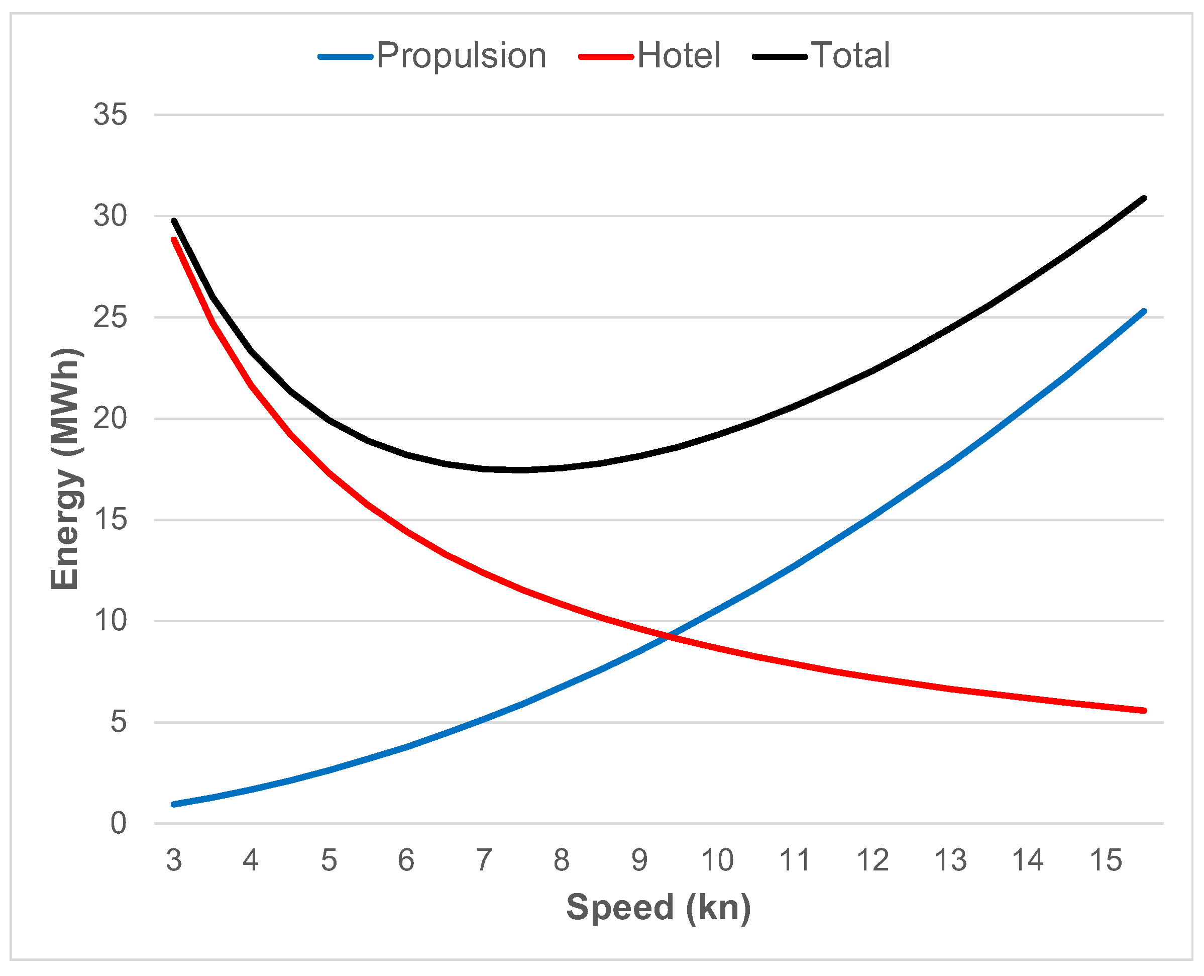
While total propulsion energy (and fuel mass) required for sailing a leg is reduced when speed is reduced, a contrary relationship holds for auxiliary energy. Slowing down increases leg sailing duration, which is multiplied by the constant 2 MW auxiliary power to calculate the total auxiliary energy. Comparing the Stockholm 80 km leg in the baseline and zero-emission Helsinki cases, auxiliary energy is 7.2 MWh in the former, where speed is 12 kn, and 8.24 MWh in the latter, where speed is 10.49 kn. Interpolating this trend further leads to a conclusion that auxiliary energy approaches infinity as speed approaches zero. In more practical terms, a shipowner faces a lower bound for the sailing speed on the zero-emission legs, battery capacity and investment cost when a constant auxiliary power is in effect.
Figure 5 illustrates the propulsion (blue trace), auxiliary (red trace) and the total (black trace) energy demand on the 80 km leg as a function of speed. The speed corresponding to the minimum total energy demand 17.5 MWh is roughly 7.5 kn. The energy demand, in this case, is lower than 20.46 and 20.68 MWh in Table 8. However, the decision to sail at the lower 7.5 kn speed would increase total costs, which is evident from the solution of the optimization problem. Nevertheless, a shipowner may prefer lower battery investment cost and higher fuel cost over the minimum total cost of the optimal choice. This decision is constrained by the 17.5 MWh lower bound of the battery capacity.
6. Conclusions
This paper presented a rigorous algorithmic decision support tool for designing and operating a ship’s energy system with environmental constraints. The problem structure gives rise to nonconvexities from binary variables and bilinear product terms. Thus, the problem is not easy to solve globally. We show that this problem belongs to a class for which non-heuristic algorithms are available. This guarantees convergence to the global optimum and supports interactive use of the tool by providing results nearly instantaneously.
The first applications of the model focused on routing, speed, and NOx compliance when sailing on routes with alternative legs inside and outside the ECA area. The original version of this problem, without zero-emission zones, has been addressed in the literature. The works were completed before the IMO 2020 global 0.5% sulfur limit came into force. Heavy fuel oil and ECA compliant low sulfur oil price difference incentivized shipowners to bypass ECAs by sailing a longer route, increasing fuel consumption and emissions. Today, the fuel switching decision is made between 0.1% and 0.5% sulfur fuels. Our results indicate that the price difference is not significant enough to justify longer routes outside ECA. Thus, we conclude that the ECA routing problem has minimal relevance nowadays.
A shipowner considering transitory battery-powered zero-emission sailing needs to evaluate the trade-off between battery investment cost and fuel cost. Namely, reducing speed in a zero-emission leg translates to lower battery capacity (and cost) but higher speed (and fuel cost) outside the zero-emission area, given that the total voyage duration is the same. The optimal trade-off is achieved by large, even 50% speed reduction in zero-emission areas. Moreover, the zero-emission legs are typically located in archipelagos, fjords, and narrow shipping lanes that enforce a 10–12 knot speed limit. In all cases studied in this work, the optimal speed is lower than the limit.
A zero-emission area can have a negative impact on total voyage GHG emissions. A shipowner, who aims to minimize total costs, benefits from reducing speed in battery-powered legs, trading off battery investment cost to fuel cost. This increases speed, energy consumption, fuel use, and emissions when sailing outside the zero-emission areas. The result is in line with previous work with respect to trading off between local NOx and total GHG emissions by propulsion power source switching [30]. Nevertheless, the improvement in local air quality may justify the increase in total emissions.
Author Contributions
Conceptualization, A.R., K.S.-T. and K.T.; methodology, A.R. and J.H.; investigation, A.R.; data curation, K.S.-T., S.N. and A.R.; writing—original draft preparation, A.R. and K.S.-T.; writing—review and editing, A.R., K.S.-T., K.T., J.H. and S.N.; visualization, A.R. and K.S.-T.; supervision, K.T. and S.N.; project administration, K.T. and S.N.; funding acquisition, K.T. and S.N. All authors have read and agreed to the published version of the manuscript.
Funding
This research was funded by Business Finland’s INTENS project 8104/31/2017.
Acknowledgments
The authors thank Tallink Silja Oy for contributing data to this study.
Conflicts of Interest
The authors declare no conflict of interest.
Abbreviations
The following abbreviations are used in this manuscript:
| CII | carbon intendity indicator |
| ECA | emission control area |
| EEDI | energy efficiency design index |
| EES | electrical energy storage |
| EEXI | energy efficiency design index for existing ships |
| EGT | exhaust gas treatment |
| GHG | greenhouse gas |
| HSFO | high sulfur fuel oil |
| IFO | intermediate fuel oil |
| LSMGO | Low sulfur marine gas oil |
| LNG | liquified natural gas |
| MS | medium speed |
| NMC | nickel manganese cobalt |
| OPS | onshore power supply |
| SCR | selective catalytic reduction |
| SFOC | specific fuel oil consumption |
| VLSFO | very low sulfur fuel oil |
References
- Sofiev, M.; Winebrake, J.; Johansson, L.; Carr, E. Cleaner fuels for ships provide public health benefits with climate tradeoffs. Nat. Commun. 2012, 406, 1–12. [Google Scholar] [CrossRef] [Green Version]
- Schwartz, H.; Gustafsson, M.; Spohr, J. Emission abatement in shipping—Is it possible to reduce carbon dioxide emissions profitably? J. Clean. Prod. 2020, 254, 120069. [Google Scholar] [CrossRef]
- Pryun, J.; van Grootheest, I.; Lafeber, F.H.; Scholtens, M. Support for selection of environmental impact abatement equipment in the early stage design. In Proceedings of the 12th Symposium on High Performance Marine Vehicles, Cortona, Italy, 12–14 October 2020; Bertram, V., Ed.; Technische Universität Hamburg: Hamburg, Germany, 2020. [Google Scholar]
- Balland, O.; Erikstad, S.O.; Fagerholt, K. Concurrent design of vessel machinery system and air emission controls to meet future air emissions regulations. Ocean Eng. 2014, 84, 283–292. [Google Scholar] [CrossRef]
- Baldi, F.; Brynolf, S.; Maréchal, F. The cost of innovative and sustainable future ship energy systems. In Proceedings of the 32nd International Conference on Efficiency, Cost, Optimization, Simulation and Environmental Impact of Energy Systems, Wrocław, Poland, 23–28 June 2019. [Google Scholar]
- Winebrake, J.J.; Corbett, J.J.; Wang, C.; Farrell, A.E.; Woods, P. Optimal Fleetwide Emissions Reductions for Passenger Ferries: An Application of a Mixed-Integer Nonlinear Programming Model for the New York–New Jersey Harbor. J. Air Waste Manag. Assoc. 2005, 55, 458–466. [Google Scholar] [CrossRef]
- Trivyza, N.L.; Rentizelas, A.; Theotokatos, G. A novel multi-objective decision support method for ship energy systems synthesis to enhance sustainability. Energy Convers. Manag. 2018, 168, 128–149. [Google Scholar] [CrossRef] [Green Version]
- Ritari, A.; Huotari, J.; Halme, J.; Tammi, K. Hybrid electric topology for short sea ships with high auxiliary power availability requirement. Energy 2020, 190, 116359. [Google Scholar] [CrossRef]
- Huotari, J.; Ritari, A.; Vepsäläinen, J.; Tammi, K. Hybrid Ship Unit Commitment with Demand Prediction and Model Predictive Control. Energies 2020, 13, 4748. [Google Scholar] [CrossRef]
- Ölçer, A.; Ballini, F. The development of a decision making framework for evaluating the trade-off solutions of cleaner seaborne transportation. Transp. Res. Part D Transp. Environ. 2015, 37, 150–170. [Google Scholar] [CrossRef]
- Hansson, J.; Månsson, S.; Brynolf, S.; Grahn, M. Alternative marine fuels: Prospects based on multi-criteria decision analysis involving Swedish stakeholders. Biomass Bioenergy 2019, 126, 159–173. [Google Scholar] [CrossRef]
- Ren, J.; Lützen, M. Fuzzy multi-criteria decision-making method for technology selection for emissions reduction from shipping under uncertainties. Transp. Res. Part D Transp. Environ. 2015, 40, 43–60. [Google Scholar] [CrossRef]
- Goldie-Scot, L. A Behind the Scenes Take on Lithium-Ion Battery Prices; Technical Report; Bloomberg New Energy Finance: New York, NY, USA, 2019. [Google Scholar]
- Solving Challenges in Energy Storage. 2018. Available online: http://www.energy.gov/sites/default/files/2019/07/f64/2018-OTT-Energy-Storage-Spotlight.pdf (accessed on 28 July 2021).
- Besselink, I.; van Oorschot, P.; Meinders, E.; Nijmeijer, H. Design of an efficient, low weight battery electric vehicle based on a VW Lupo 3L. In Proceedings of the 25th World Battery, Hybrid and Fuel Cell Electric Vehicle Symposium & Exhibition (EVS-25), Shenzhen, China, 5–9 November 2010. [Google Scholar]
- Finnlines. Hybrid ro-ro Vessels Sail into a Green Future. 2020. Available online: https://www.finnlines.com/company/news-stories/finnlines-news-22020/hybrid-ro-ro-vessels-sail-green-future (accessed on 6 August 2021).
- Motorship. Havila Kystruten Ferries to Feature 6.1 MWh Corvus ESS. 2019. Available online: https://www.motorship.com/news101/industry-news/havila-kystruten-ferries-to-feature-6.1mwh-corvus-batteries (accessed on 6 August 2021).
- IMO. Prevention of Air Pollution From Ships. 2020. Available online: http://www.imo.org/en/OurWork/Environment/PollutionPrevention/AirPollution/Pages/Air-Pollution.aspx (accessed on 20 July 2021).
- Commission, E. Emission Trading—Putting a Price on Carbon. 2021. Available online: https://ec.europa.eu/commission/presscorner/detail/en/qanda_21_3542 (accessed on 20 July 2021).
- Wärtsilä Environmental Product Guide. 2017. Available online: http://cdn.wartsila.com/docs/default-source/product-files/egc/product-guide-o-env-environmental-solutions.pdf (accessed on 28 July 2021).
- Solakivi, T.; Laari, S.; Kiiski, T.; Töyli, J.; Ojala, L. How shipowners have adapted to sulphur regulations—Evidence from Finnish seaborne trade. Case Stud. Transp. Policy 2019, 7, 338–345. [Google Scholar] [CrossRef]
- Li, K.; Wu, M.; Gu, X.; Yuen, K.F.; Xiao, Y. Determinants of ship operators’ options for compliance with IMO 2020. Transp. Res. Part D Transp. Environ. 2020, 86, 102459. [Google Scholar] [CrossRef]
- Bektaş, T.; Ehmke, J.F.; Psaraftis, H.N.; Puchinger, J. The role of operational research in green freight transportation. Eur. J. Oper. Res. 2019, 274, 807–823. [Google Scholar] [CrossRef] [Green Version]
- Fagerholt, K.; Gausel, N.T.; Rakke, J.G.; Psaraftis, H.N. Maritime routing and speed optimization with emission control areas. Transp. Res. Part C Emerg. Technol. 2015, 52, 57–73. [Google Scholar] [CrossRef] [Green Version]
- Geertsma, R.; Negenborn, R.; Visser, K.; Hopman, J. Design and control of hybrid power and propulsion systems for smart ships: A review of developments. Appl. Energy 2017, 194, 30–54. [Google Scholar] [CrossRef]
- Thanh Long, V.; Dhupia, J.; Alexander, A.; Kennedy, L.; Adnanes, A. Control optimization for electric tugboats powertrain with a given load profile. In Proceedings of the ISCIE/ASME International Symposium on Flexible Automation, Awaji-Island, Hyōgo, Japan, 14–16 July 2014. [Google Scholar]
- Jaurola, M.; Hedin, A.; Tikkanen, S.; Huhtala, K. TOpti: A flexible framework for optimising energy management for various ship machinery topologies. J. Mar. Sci. Technol. 2018, 24, 1183–1196. [Google Scholar] [CrossRef] [Green Version]
- Pyrhönen, O.; Pinomaa, A.; Lindh, T.; Peltoniemi, P.; Lana, A.; Montonen, H.; Tikkanen, K. Future Energy Storage Solutions in Marine Installations–FESSMI–Final Report; University of Vaasa: Vaasa, Finland, 2017. [Google Scholar]
- Dedes, E. Investigation of Hybrid Systems for Diesel Powered Ships. Ph.D. Thesis, University of Southampton, Southampton, UK, 2013. [Google Scholar]
- Sui, C.; de Vos, P.; Stapersma, D.; Visser, K.; Ding, Y. Fuel Consumption and Emissions of Ocean-Going Cargo Ship with Hybrid Propulsion and Different Fuels over Voyage. J. Mar. Sci. Eng. 2020, 8, 588. [Google Scholar] [CrossRef]
- Sui, C.; de Vos, P.; Stapersma, D.; Visser, K.; Ding, Y. Impact of Battery-Hybrid Cargo Ship Propulsion on Fuel Consumption and Emissions during Port Approaches. In Proceedings of the CIMAC Congress 2019, Vancouver, BC, Canada, 10–12 June 2019. [Google Scholar]
- Psaraftis, H.N.; Kontovas, C.A. Ship speed optimization: Concepts, models and combined speed-routing scenarios. Transp. Res. Part C Emerg. Technol. 2014, 44, 52–69. [Google Scholar] [CrossRef] [Green Version]
- Misener, R.; Floudas, C.A. GloMIQO: Global mixed-integer quadratic optimizer. J. Glob. Optim. 2012, 57, 3–50. [Google Scholar] [CrossRef] [Green Version]
- Achterberg, T.; Towle, E. Non-Convex Quadratic Optimization. 2020. Available online: https://www.gurobi.com/resource/non-convex-quadratic-optimization/ (accessed on 23 August 2021).
- Schuller, O.; Kupferschmid, S.; Hengstler, J.; Whitehouse, S. Life Cycle GHG Emission Study on the Use of LNG as Marine Fuel; Hinkstep: Stuttgart, Germany, 2019. [Google Scholar]
- Well-to-Wheels Report Version 4.a: JEC Well to Wheels Analysis—Well to Wheels Analysis of Future Automotive Fuels and Powertrains in the European Context; European Commission Joint Research Centre Institute for Energy and Transport: Brussels, Belgium, 2014. [CrossRef]
- Jalkanen, J.P.; Johansson, L.; Kukkonen, J.; Brink, A.; Kalli, J.; Stipa, T. Extension of an assessment model of ship traffic exhaust emissions for particulate matter and carbon monoxide. Atmos. Chem. Phys. 2012, 12, 2641–2659. [Google Scholar] [CrossRef] [Green Version]
- Brynolf, S.; Magnusson, M.; Fridell, E.; Andersson, K. Compliance possibilities for the future ECA regulations through the use of abatement technologies or change of fuels. Transp. Res. Part D Transp. Environ. 2014, 28, 6–18. [Google Scholar] [CrossRef]
- Anderson, M.; Salo, K.; Fridell, E. Particle- and Gaseous Emissions from an LNG Powered Ship. Environ. Sci. Technol. 2015, 49, 12568–12575. [Google Scholar] [CrossRef]
- Willems, F.; Modeling & Control of Diesel Aftertreatment Systems. 1st International TNO—TU/e—LiU Course. 2015. Available online: https://www.fs.isy.liu.se/Edu/Courses/AftertreatmentMaC/Exercise_10_solution.pdf (accessed on 28 August 2021).
- Lahtinen, J. Closed-Loop Exhaust Gas Scrubber Onboard a Merchant Ship—Technical, Economical, Environmental and Operational Viewpoints. Ph.D. Thesis, University of Vaasa, Vaasa, Finland, 2015. [Google Scholar]
- Myhre, G.; Shindell, D.; Bréon, F.M.; Collins, W.; Fuglestvedt, J.; Huang, J.; Koch, D.; Lamarque, J.F.; Lee, D.; Mendoza, B.; et al. Anthropogenic and natural radiative forcing. In Climate Change 2013: The Physical Science Basis. Contribution of Working Group I to the Fifth Assessment Report of the Intergovernmental Panel on Climate Change; Stocker, T.F., Qin, D., Plattner, G.K., Tignor, M., Allen, S.K., Doschung, J., Nauels, A., Xia, Y., Bex, V., Midgley, P.M., Eds.; Cambridge University Press: Cambridge, UK, 2013; pp. 659–740. [Google Scholar] [CrossRef]
- Exhaust Gas Cleaning Systems Association. A Practical Guide to Exhaust Gas Cleaning Systems for the Maritime Industry; Exhaust Gas Cleaning Systems Association: Staines, UK, 2012. [Google Scholar]
- European Commission. Covenant of Mayors for Climate and Energy: Default Emission Factors for Local Emission Inventories: Version 2017; European Commission Publications Office: Brussels, Belgium, 2017. [Google Scholar] [CrossRef]
- DieselNet Technology Guide. 2021. Available online: https://dieselnet.com/tg.php (accessed on 28 July 2021).
- Winnes, H.; Fridell, E. Particle Emissions from Ships: Dependence on Fuel Type. J. Air Waste Manag. Assoc. 2009, 59, 1391–1398. [Google Scholar] [CrossRef]
- Your Options for Emissions Compliance. Guidance for Shipowners and Operators on the Annex VI SOx and NOx Regulations; Lloyd’s Register: London, UK, 2015. [Google Scholar]
- Ship Technology. Debunking: The Problem of Ships Using Open-Loop Scrubbers. 2021. Available online: https://www.ship-technology.com/features/open-loop-scubbers/ (accessed on 21 July 2021).
- den Boer, E.; Hoen, M. Scrubbers—An Economic and Ecological Assessment. 2015. Available online: https://www.nabu.de/downloads/150312-Scrubbers.pdf (accessed on 28 August 2021).
- Bacher, H.; Albrecht, P. Evaluating the costs arising from new maritime environmental regulations. Trafi Publ. 2013, 24, 2013. [Google Scholar]
- Spoof-Tuomi, K. Calculation Tool for Profitability Assessment of SOx Scrubber Investments. Barchelor’s Thesis, University of Applied Sciences, Vaasa, Finland, 2013. [Google Scholar]
- IACCSEA. Marine SCR—Cost Benefit Analysis. 2013. Available online: https://www.iaccsea.com/wp-content/uploads/2018/12/IACCSEA-Marine-SCR-Cost-benefit-analysis-2013.pdf (accessed on 28 August 2021).
- Zheng, G.; Wang, F.; Wang, S.; Gao, W.; Zhao, Z.; Liu, J.; Wang, L.; Wu, L.; Wang, H. Urea SCR System Development for Large Diesel Engines; SAE Technical Paper Series; SAE International: Warrendale, PA, USA, 2014. [Google Scholar] [CrossRef]
- MAN Energy Solutions. MAN 32/44CR Project Guide; MAN Energy Solutions: Augsburg, Germany, 2019. [Google Scholar]
- Wik, C.; Niemi, S. Low emission engine technologies for future tier 3 legislations—Options and case studies. J. Shipp. Trade 2016, 1, 1–22. [Google Scholar] [CrossRef] [Green Version]
- Issa, M.; Ibrahim, H.; Ilinca, A.; Hayyani, M.Y. A Review and Economic Analysis of Different Emission Reduction Techniques for Marine Diesel Engines. Open J. Mar. Sci. 2019, 9, 148–171. [Google Scholar] [CrossRef] [Green Version]
- Yaramenka, K.; Winnes, H.; Åström, S.; Fridell, E. Cost-Benefit Analysis of NOX Control for Ships in the Baltic Sea and the North Sea; Technical Report Report C 228; IVL Swedish Environmental Research Institute: Stockholm, Sweden, 2017. [Google Scholar]
- Austin, C.; Macdonald, F.; Rojon, I. The Ship Operator’s Guide to NOx Reduction; Fathom: Windsor, UK, 2015. [Google Scholar]
- Ship and Bunker. Rotterdam Bunker Prices. 2021. Available online: https://shipandbunker.com/prices/emea/nwe/nl-rtm-rotterdam#IFO380 (accessed on 21 July 2021).
- DNV GL. Current Price Development Oil and Gas. 2021. Available online: https://www.dnvgl.com/maritime/lng/current-price-development-oil-and-gas.html (accessed on 21 July 2021).
- Statistics Finland. Energy Prices. Available online: http://www.stat.fi/til/ehi/tau_en.html (accessed on 21 July 2021).
- Dinger, A.; Martin, R.; Mosquet, X.; Rizoulis, D.; Russo, M.; Sticher, G. Batteries for Electric Cars: Challenges, Opportunities, and the Outlook to 2020; Technical Report; Boston Consulting Group: Boston, MA, USA, 2010. [Google Scholar]
- McKinsey. Electrifying Insights: How Automakers Can Drive Electrified Vehicle Sales and Profitability; McKinsey: Atlanta, GA, USA, 2017. [Google Scholar]
Figure 1.
Construction of alternative routes from a set of sailing legs.

Figure 2.
Price development of intermediate fuel oil (IFO) 380, 0.1% sulfur marine gas oil (MGO) and European Union (EU) natural gas from 1 August 2014 to 1 February 2021. The source price data in the unit $/mmBTU from [60] has been converted to EUR/GJ with USD to EUR exchange rate 0.943 and 1 mmBTU = 1.06 GJ.
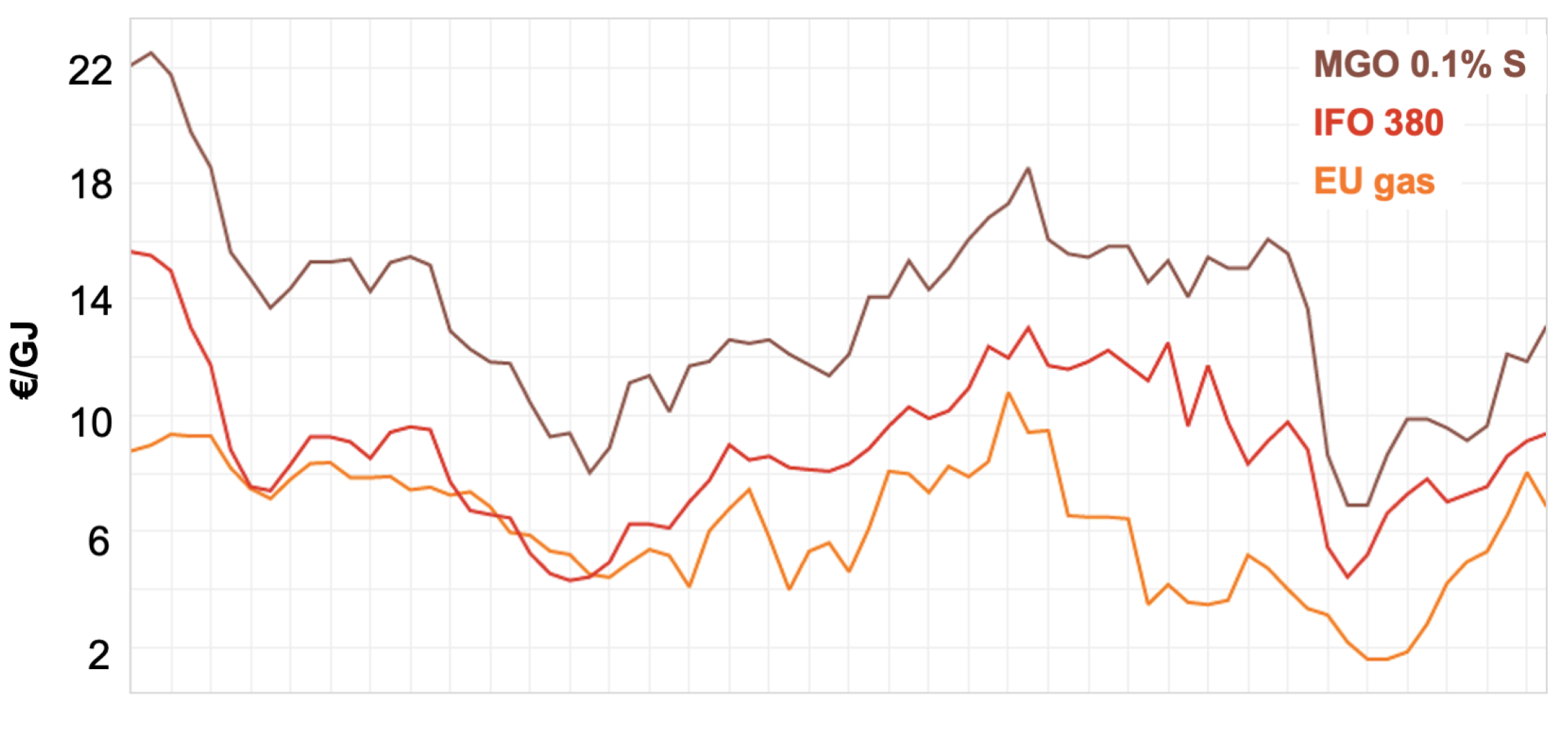
Figure 3.
Map of the route from Florø to Nantes and the alternative legs in the North Sea. ECA border is shown as light blue in the North Sea and the English channel. The red cones represent 10 km port arrival and departure legs which may be designated as zero-emission areas [9]. Background satellite image by Google.

Figure 4.
Map of the Baltic Sea routes. Background satellite image by NASA.
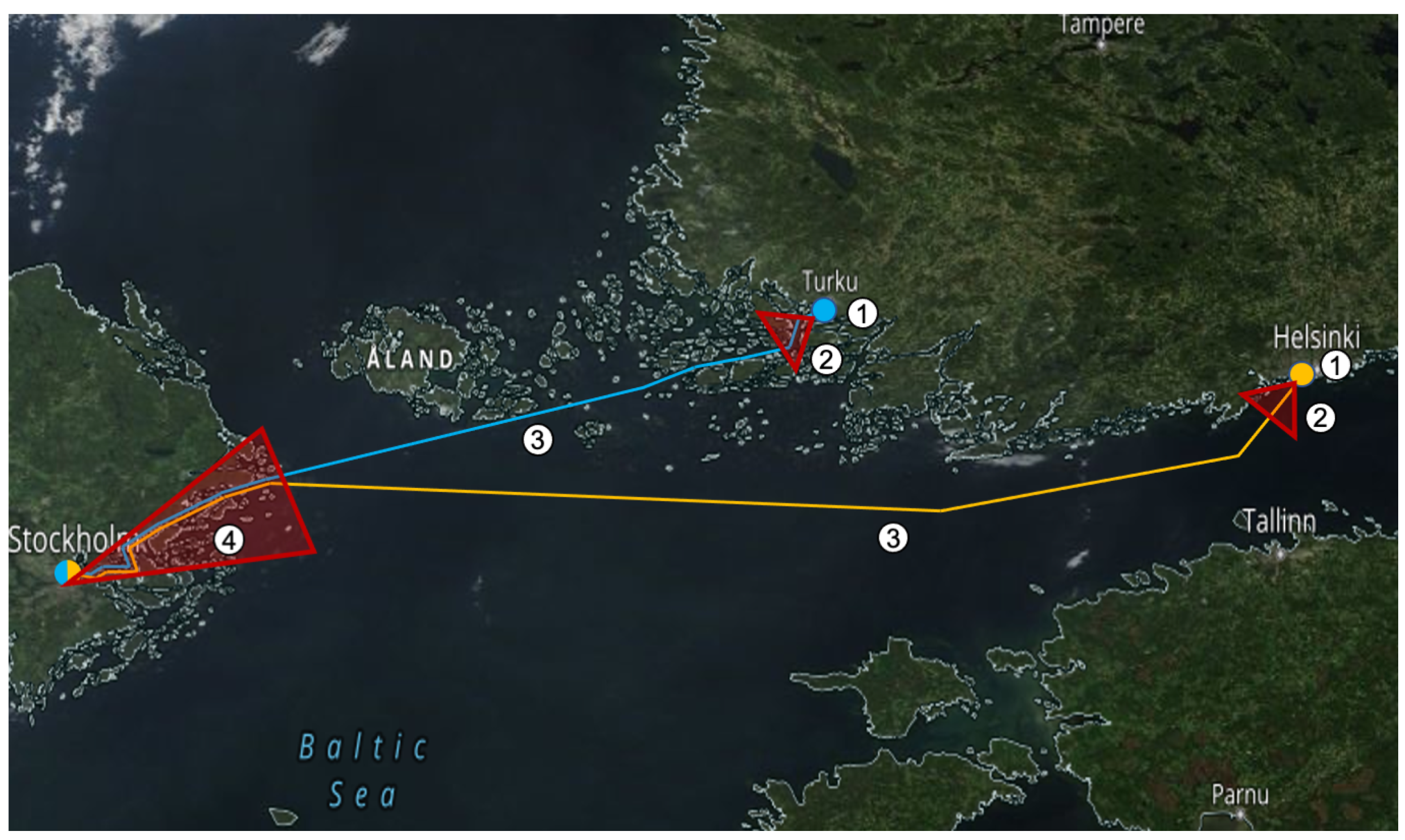
Figure 5.
Total energy demand on the Stockholm archipelago leg as a function of speed.

Table 1.
Model notation. EGT stands for exhaust gas treatment.
| Indexing | |
| Number of fuels | |
| Number of pollutant types | |
| Number of engine types | |
| Number of exhaust gas treatment unit types | |
| Number of sailing legs | |
| Number of routes | |
| Variables | |
| Speed on legs (km/h) | |
| Sailing duration on legs (h) | |
| Power output from use of fuels on legs (MWh) | |
| Utilization rate of EGT units on legs (MWh) | |
| Battery charge on legs (MWh) | |
| Battery capacity (MWh) | |
| Charged energy to battery on legs (MWh) | |
| Discharged energy from battery on legs (MWh) | |
| Energy drawn from onshore power supply on legs (MWh) | |
| Decision to install engines | |
| Decision to install EGT units | |
| Decision to sail on routes | |
| Parameters | |
| Allocation of legs to routes | |
| Mapping between fuels and pollutants (kg/MWh) | |
| Compatibility of fuels with engines | |
| Reduction of pollutant streams in EGTs (kg/MWh) | |
| Specific pollutant limits on legs (kg/MWh) | |
| Lower heating values of fuels (MWh/ton) | |
| Electricity consumption of EGT units (%/100) | |
| Leg distance (km) | |
| Onshore power supply availability | |
| Engine investment costs (EUR) | |
| EGT investment costs (EUR) | |
| EGT operating costs (EUR/MWh) | |
| Fuel prices (EUR/ton) | |
| Battery investment cost (EUR/MWh) | |
| Onshore power supply electricity cost (EUR/MWh) | |
| Total voyage duration (h) | |
| Auxiliary electric power (MW) | |
| Hull resistance coefficient | |
| Battery charging and discharging efficiency | |
| Engine efficiency | |
| Investment cost scaling factor |
Table 2.
Specific emission factors for greenhouse gas (GHG) emissions and local pollutants at cruising load (85%). Fuel options are high sulfur fuel oil (HSFO), marine gas oil (MGO), liquified natural gas (LNG). Greenhouse gases are carbon dioxide (CO2), methane (CH4) and nitrous oxide (N2O). Local pollutants are sulfur oxides (SOx) and nitrogen dioxide (NO2). EGT stands for exhaust gas treatment and means that both a scrubber and selective catalytic reduction (SCR) system are installed. SFOC stands for specific fuel oil consumption.
| HSFO | HSFO + EGT | MGO | MGO + SCR | LNG | Source | |
|---|---|---|---|---|---|---|
| Well-to-tank GHG | ||||||
| CO2 (g/MJ fuel) | 13.2 | 13.2 | 14.1 | 14.1 | 13.7 | [35,36] |
| CH4 (g/MJ fuel) | 0.028 | 0.028 | 0.028 | 0.028 | 0.15 | [35,36] |
| CO2-eq (g/MJ fuel) | 14.2 | 14.2 | 15.1 | 15.1 | 18.8 | |
| Combustion GHG | ||||||
| CO2 (g/kWh) | 564 | 570 | 551 | 551 | 416 | [37] |
| CH4 (mg/kWh) | 4 | 4 | 4 | 4 | 1000 | [38,39] |
| N2O (mg/kWh) | 31 | 31 | 27 | 27 | 17 | [35] |
| CO2-eq (g/kWh) | 573 | 581 | 560 | 560 | 456 | |
| Local pollutants | ||||||
| NOx (g/kWh) | 11.7 | 2.0 | 9.6 | 1.9 | 1.7 | [38,39] |
| SO2 (g/kWh) | 8.11 | 0.17 | 0.34 | 0.34 | 0.01 | [35] |
| Inputs to propulsion | ||||||
| SFOC (g/kWh) | 181 | 184 | 172 | 172 | [37] | |
| Natural gas (g/kWh) | 149 | [39] | ||||
| Pilot fuel (g/kWh) | 2.1 | [39] | ||||
| Urea 100% (g/kWh) | 6.3 | 5.0 | [40] | |||
| NaOH 50% (g/kWh) | 17.5 | [41] |
Table 3.
Prices of fuel grades from the Port of Rotterdam and onshore power supply electricity from the Port of Helsinki.
Table 3.
Prices of fuel grades from the Port of Rotterdam and onshore power supply electricity from the Port of Helsinki.
| Type | Abbreviation | Sulfur (%) | Price | Source |
|---|---|---|---|---|
| High sulfur fuel oil | HSFO | 3.5 | 386 EUR/ton | [59] |
| Very low sulfur fuel oil | VLSFO | 0.5 | 505 EUR/ton | [59] |
| Low sulfur marine gas oil | LSMGO | 0.1 | 560 EUR/ton | [59] |
| Liquified natural gas | LNG | 0 | 378–733 EUR/ton | [59] |
| Electricity | OPS | 0 | 84.8 EUR/MWh | [61] |
Table 4.
Performance and cost data of energy conversion, storage and exhaust gas cleaning units. MS stands for medium speed and for efficiency.
Table 4.
Performance and cost data of energy conversion, storage and exhaust gas cleaning units. MS stands for medium speed and for efficiency.
| Unit Type | (%) | Investment | Operation | Source |
|---|---|---|---|---|
| MS diesel engine | 45 | 240 EUR/kW | [5] | |
| MS dual fuel engine | 45 | 470 EUR/kW | [5] | |
| Li-ion battery | 97 | 400 EUR/kWh | [28,63] | |
| Closed loop scrubber | 375 EUR/kW | 6 EUR/MWh | [49] | |
| SCR system | 46 EUR/kW | 3.5 EUR/MWh | [50] |
Table 5.
Baseline solution of the North Sea route. EGT stands for exhaust gas treatment. The column headers denote leg identifiers.
Table 5.
Baseline solution of the North Sea route. EGT stands for exhaust gas treatment. The column headers denote leg identifiers.
| 1 | 2 | 3 | 4 | 5 | 6 | 7 | 8 | |
|---|---|---|---|---|---|---|---|---|
| Speed, kn | 0.0 | 17.91 | 0.0 | 0.0 | 0.0 | 17.91 | 17.94 | 17.9 |
| Time, h | 0.0 | 0.3 | 0.0 | 0.0 | 0.0 | 49.86 | 10.54 | 0.3 |
| Power, MW | 0.0 | 14.03 | 0.0 | 0.0 | 0.0 | 14.04 | 14.1 | 14.02 |
| HSFO, MWh | 0.0 | 4.88 | 0.0 | 0.0 | 0.0 | 807.82 | 170.38 | 4.88 |
| VLSFO, MWh | 0.0 | 0.0 | 0.0 | 0.0 | 0.0 | 0.0 | 0.0 | 0.0 |
| LSMGO, MWh | 0.0 | 0.0 | 0.0 | 0.0 | 0.0 | 0.0 | 0.0 | 0.0 |
| LNG, MWh | 0.0 | 0.0 | 0.0 | 0.0 | 0.0 | 0.0 | 0.0 | 0.0 |
| EGT-S, MWh | 0.0 | 4.88 | 0.0 | 0.0 | 0.0 | 807.82 | 150.34 | 4.88 |
| EGT-N, MWh | 0.0 | 4.88 | 0.0 | 0.0 | 0.0 | 807.82 | 0.0 | 4.88 |
| Obj, kEUR | 99.5 | |||||||
| CO2-eq, ton | 588.82 |
Table 6.
Solution of the North Sea route with zero-emission port departure and arrival. ESS stands for electrical energy storage (battery) and OPS for onshore power supply.
Table 6.
Solution of the North Sea route with zero-emission port departure and arrival. ESS stands for electrical energy storage (battery) and OPS for onshore power supply.
| 1 | 2 | 3 | 4 | 5 | 6 | 7 | 8 | |
|---|---|---|---|---|---|---|---|---|
| Speed, kn | 0.0 | 9.52 | 0.0 | 0.0 | 0.0 | 18.07 | 18.1 | 9.52 |
| Time, h | 0.0 | 0.57 | 0.0 | 0.0 | 0.0 | 49.42 | 10.44 | 0.57 |
| Power, MW | 0.0 | 2.1 | 0.0 | 0.0 | 0.0 | 14.42 | 14.49 | 2.11 |
| HSFO, MWh | 0.0 | 0.0 | 0.0 | 0.0 | 0.0 | 819.52 | 175.38 | 0.0 |
| VLSFO, MWh | 0.0 | 0.0 | 0.0 | 0.0 | 0.0 | 0.0 | 0.0 | 0.0 |
| LSMGO, MWh | 0.0 | 0.0 | 0.0 | 0.0 | 0.0 | 0.0 | 0.0 | 0.0 |
| LNG, MWh | 0.0 | 0.0 | 0.0 | 0.0 | 0.0 | 0.0 | 0.0 | 0.0 |
| ESS (—), MWh | 0.0 | 2.4 | 0.0 | 0.0 | 0.0 | 0.0 | 0.0 | 2.4 |
| ESS (+), MWh | 2.4 | 0.0 | 0.0 | 0.0 | 0.0 | 0.01 | 2.39 | 0.0 |
| OPS, MWh | 2.48 | 0.0 | 0.0 | 0.0 | 0.0 | 0.0 | 0.0 | 0.0 |
| EGT-S, MWh | 0.0 | 0.0 | 0.01 | 0.01 | 0.01 | 819.52 | 154.75 | 0.0 |
| EGT-N, MWh | 0.0 | 0.0 | 0.0 | 0.01 | 0.0 | 819.52 | 0.0 | 0.0 |
| Obj, kEUR | 104.05 | |||||||
| CO2-eq, ton | 593.47 |
Table 7.
Baseline solutions of the Baltic Sea routes.
| Helsinki | Turku | |||||||
|---|---|---|---|---|---|---|---|---|
| 1 | 2 | 3 | 4 | 1 | 2 | 3 | 4 | |
| Speed, kn | 0.0 | 16.54 | 16.58 | 12.0 | 0.0 | 16.38 | 16.37 | 12.0 |
| Time, h | 0.0 | 0.33 | 11.07 | 3.6 | 0.0 | 0.33 | 6.07 | 3.6 |
| Power, MW | 0.0 | 11.06 | 11.13 | 4.22 | 0.0 | 10.74 | 10.71 | 4.22 |
| HSFO, MWh | 0.0 | 0.0 | 0.0 | 0.0 | 0.0 | 0.0 | 0.0 | 0.0 |
| VLSFO, MWh | 0.0 | 0.0 | 0.0 | 0.0 | 0.0 | 0.0 | 0.0 | 0.0 |
| LSMGO, MWh | 0.0 | 4.28 | 146.15 | 22.51 | 0.0 | 4.22 | 77.54 | 22.51 |
| LNG, MWh | 0.0 | 0.0 | 0.0 | 0.0 | 0.0 | 0.0 | 0.0 | 0.0 |
| EGT-S, MWh | 0.0 | 0.0 | 0.0 | 0.0 | 0.0 | 0.0 | 0.0 | 0.0 |
| EGT-N, MWh | 0.0 | 4.29 | 146.15 | 22.51 | 0.0 | 4.22 | 77.54 | 22.51 |
| Obj, kEUR | 21.96 | 15.26 | ||||||
| CO2-eq, ton | 101.0 | 60.9 | ||||||
Table 8.
Solutions of the Baltic Sea routes with zero-emission port arrival and departure.
| Helsinki | Turku | ||||||||
|---|---|---|---|---|---|---|---|---|---|
| 1 | 2 | 3 | 4 | 1 | 2 | 3 | 4 | ||
| Speed, kn | 0.0 | 17.44 | 17.37 | 10.49 | 0.0 | 17.16 | 17.66 | 10.64 | |
| Time, h | 0.0 | 0.31 | 10.57 | 4.12 | 0.0 | 0.31 | 5.62 | 4.06 | |
| Power, MW | 0.0 | 12.96 | 12.79 | 2.82 | 0.0 | 12.35 | 13.47 | 2.94 | |
| HSFO, MWh | 0.0 | 0.0 | 0.0 | 0.0 | 0.0 | 0.0 | 0.0 | 0.0 | |
| VLSFO, MWh | 0.0 | 0.0 | 0.0 | 0.0 | 0.0 | 0.0 | 0.0 | 0.0 | |
| LSMGO, MWh | 0.0 | 0.0 | 162.13 | 0.0 | 0.0 | 0.0 | 92.25 | 0.0 | |
| LNG, MWh | 0.0 | 0.0 | 0.0 | 0.0 | 0.0 | 0.0 | 0.0 | 0.0 | |
| EES (—), MWh | 0.0 | 4.78 | 0.0 | 20.46 | 0.0 | 4.65 | 0.0 | 20.68 | |
| EES (+), MWh | 20.46 | 0.0 | 4.78 | 0.0 | 20.68 | 0.0 | 4.65 | 0.0 | |
| OPS, MWh | 21.09 | 0.0 | 0.0 | 0.0 | 21.32 | 0.0 | 0.0 | 0.0 | |
| EGT-S, MWh | 0.0 | 0.0 | 0.0 | 0.0 | 0.0 | 0.0 | 0.0 | 0.0 | |
| EGT-N, MWh | 0.0 | 0.0 | 162.13 | 0.0 | 0.0 | 0.0 | 92.25 | 0.0 | |
| Obj, kEUR | 33.51 | 26.83 | |||||||
| CO2-eq, ton | 97.75 | 58.27 | |||||||
Publisher’s Note: MDPI stays neutral with regard to jurisdictional claims in published maps and institutional affiliations. |
© 2021 by the authors. Licensee MDPI, Basel, Switzerland. This article is an open access article distributed under the terms and conditions of the Creative Commons Attribution (CC BY) license (https://creativecommons.org/licenses/by/4.0/).
Share and Cite
MDPI and ACS Style
Ritari, A.; Spoof-Tuomi, K.; Huotari, J.; Niemi, S.; Tammi, K. Emission Abatement Technology Selection, Routing and Speed Optimization of Hybrid Ships. J. Mar. Sci. Eng. 2021, 9, 944. https://doi.org/10.3390/jmse9090944
AMA Style
Ritari A, Spoof-Tuomi K, Huotari J, Niemi S, Tammi K. Emission Abatement Technology Selection, Routing and Speed Optimization of Hybrid Ships. Journal of Marine Science and Engineering. 2021; 9(9):944. https://doi.org/10.3390/jmse9090944
Chicago/Turabian StyleRitari, Antti, Kirsi Spoof-Tuomi, Janne Huotari, Seppo Niemi, and Kari Tammi. 2021. "Emission Abatement Technology Selection, Routing and Speed Optimization of Hybrid Ships" Journal of Marine Science and Engineering 9, no. 9: 944. https://doi.org/10.3390/jmse9090944
Note that from the first issue of 2016, this journal uses article numbers instead of page numbers. See further details here.