
Numerical Modelling of Oil Spill Transport in Tide-Dominated Estuaries: A Case Study of Humber Estuary, UK

 , , , and
Abstract
:1. Introduction
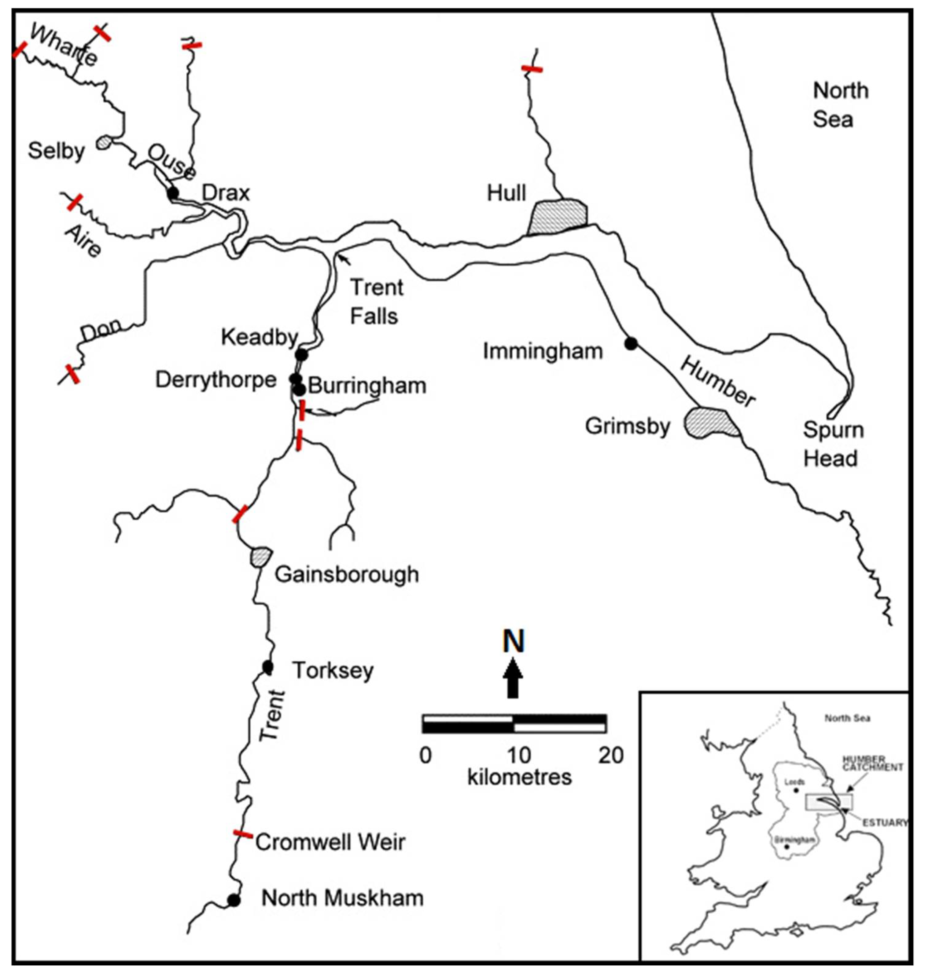
2. Study Area
3. Materials and Methods
3.1. Hydrodynamic Model
3.2. Oil Trajectory Model
3.3. Calibration and Validation Design
3.3.1. River Discharge
3.3.2. Model Calibration and Validation Scenarios
3.4. Oil Spill Simulation Design
3.4.1. River Discharge Scenarios
3.4.2. Wind Data for Oil Spill Scenarios
4. Result
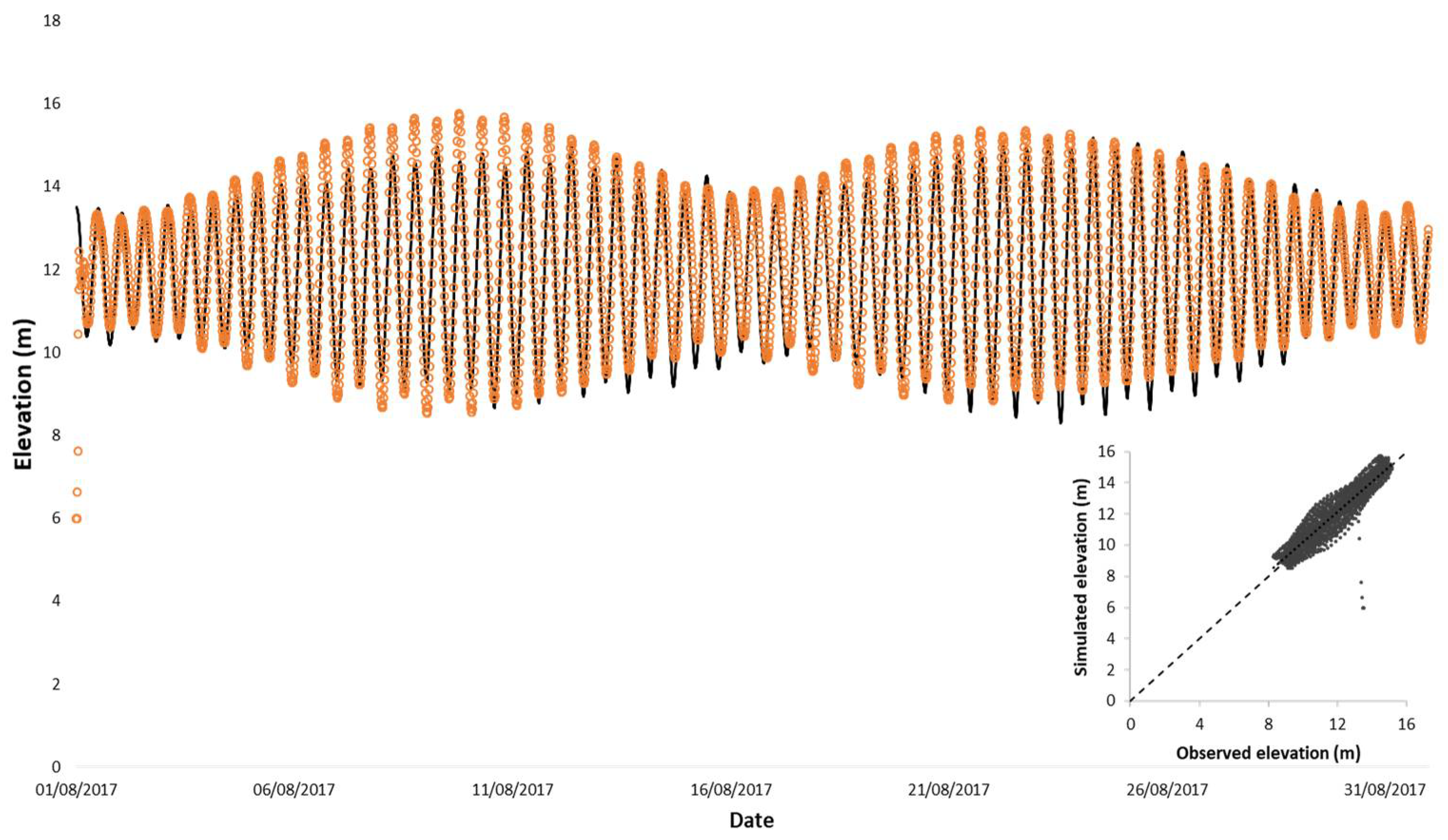
4.1. Calibration and Validation
4.1.1. Calibration
4.1.2. Validation
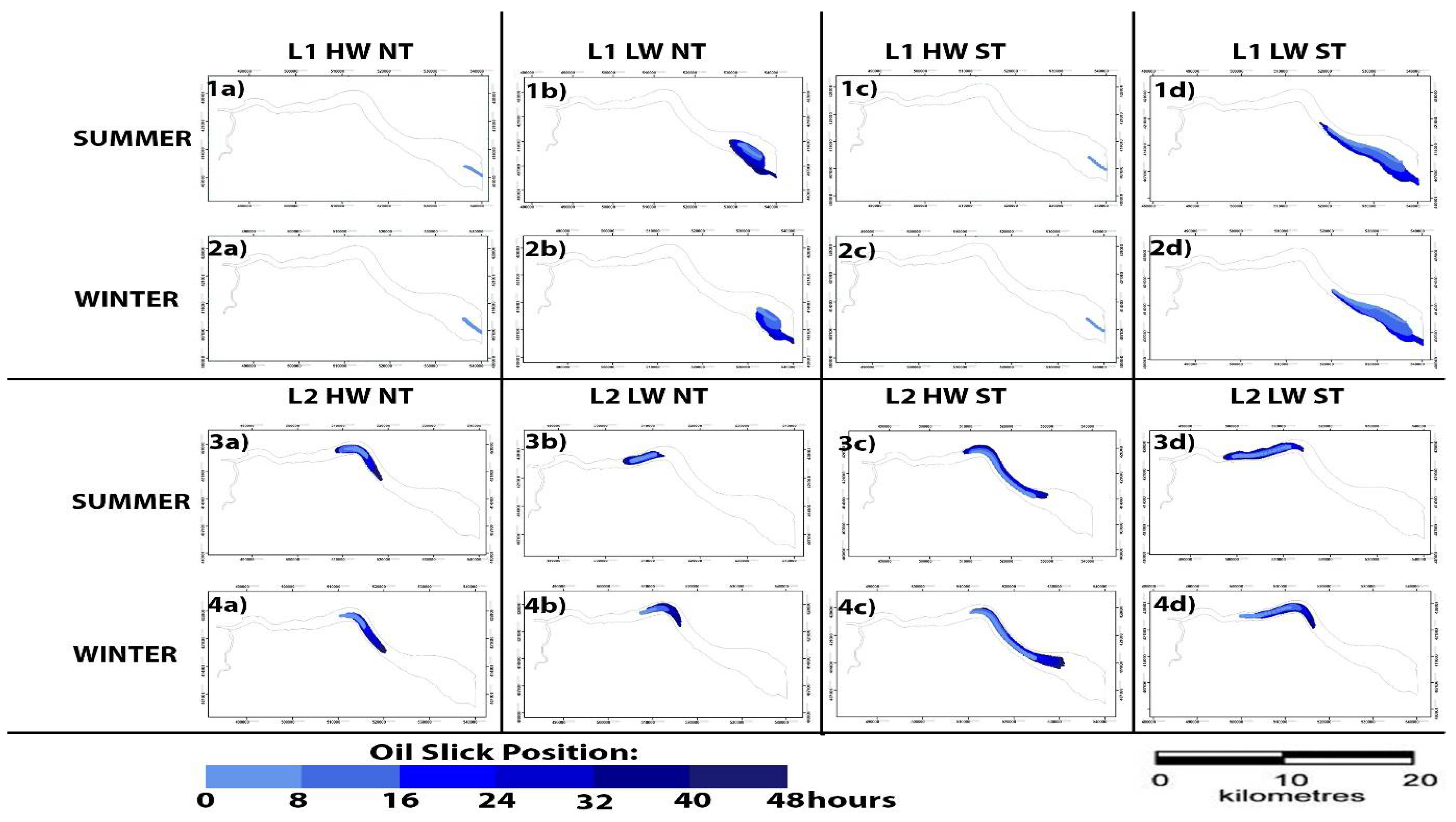
4.2. Oil Spill Scenarios
5. Discussion
5.1. Impact of River Discharge Variation: Summer (Low River Discharge) vs. Winter (High River Discharge)
5.2. Impact of Tide (Spring Tide vs. Neap Tide)
5.3. Impact of Tidal Stage (High Water vs. Low Water)
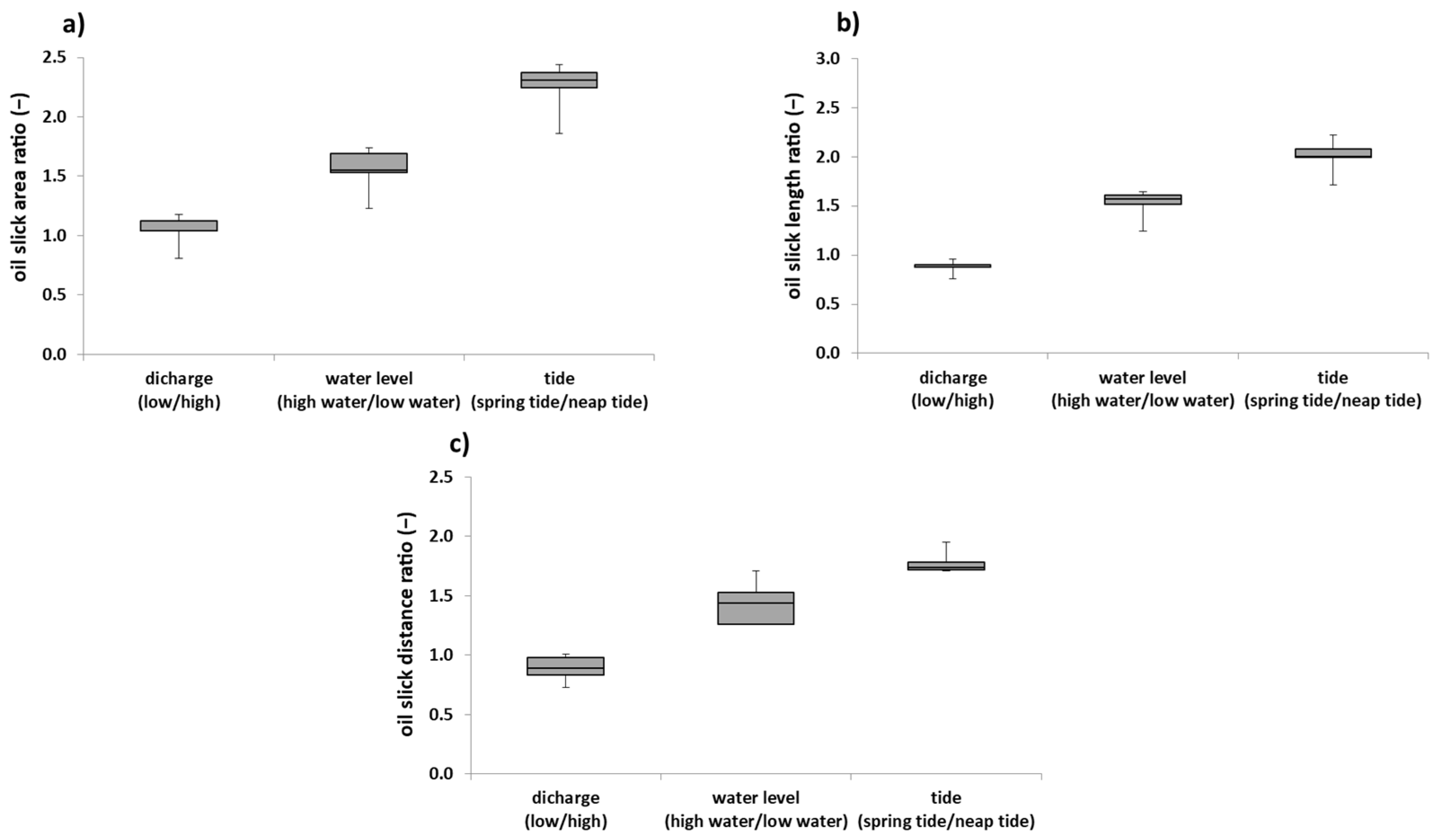
5.4. Relative Impacts of River Discharge vs. Tide vs. Stage
5.5. Influence of Oil Spill Release Location
5.6. Oil Beaching
6. Conclusions
- because of variation in river discharge, slicks released under high river discharge at high water did not exhibit any upstream displacement over repeated tidal cycles, while slicks released under low river discharge travelled upstream into the estuary over repeated tidal cycles;
- there is a statistically significant (p < 0.05) difference in the influence of hydrodynamic conditions (river discharge variation, water level and tidal range) on oil slick impacted area, length and distance travelled;
- the tidal range has a key influence on oil slick impacted area, with spring tide slicks being 125% bigger than neap tide slicks, on average;
- oil slick impacted area, length and distance travelled is predominantly affected by the tidal range (i.e., spring or neap) at the time of oil release, and only then by the stage or river discharge;
- the influence of river discharge on oil slick spreading is dependent on the time of release within a tidal cycle; and
- the possibility of oil beaching on the banks of the estuary exposes environmental risks, with up to 24.6 km of shoreline affected in our simulations.
Supplementary Materials
Author Contributions
Funding
Institutional Review Board Statement
Informed Consent Statement
Data Availability Statement
Acknowledgments
Conflicts of Interest
References
- Kim, Y.H.; Hong, S.; Song, Y.S.; Lee, H.; Kim, H.; Ryu, J.; Park, J.; Kwon, B.; Lee, C.; Khim, J.S. Seasonal Variability of Estuarine Dynamics due to Freshwater Discharge and its Influence on Biological Productivity in Yeongsan River Estuary, Korea. Chemosphere 2017, 181, 390–399. [Google Scholar] [CrossRef]
- McLusky, D.S.; Elliott, M. The Estuarine Ecosystem: Ecology, Threats and Management, 3rd ed.; Oxford University Press: New York, NY, USA, 2004. [Google Scholar]
- Rehitha, T.V.; Ullas, N.; Vineetha, G.; Benny, P.Y.; Madhu, N.V.; Revichandran, C. Impact of Maintenance Dredging on Macrobenthic Community Structure of a Tropical Estuary. Ocean. Coast. Manag. 2017, 144, 71–82. [Google Scholar] [CrossRef]
- Woodroffe, C.D.; Nicholls, R.J.; Saito, Y.; Chen, Z.; Goodbred, S.L. Landscape Variability and the Response of Asian Megadeltas to Environmental Change. In Global Change and Integrated Coastal Management; Springer: AnonDordrecht, The Netherlands, 2006; Volume 10, pp. 277–314. [Google Scholar]
- Syvitski, J.P.M.; Saito, Y. Morphodynamics of Deltas Under the Influence of Humans. Glob. Planet. Chang. 2007, 57, 261–282. [Google Scholar] [CrossRef]
- Pezy, J.; Baffreau, A.; Dauvin, J. What are the Factors Driving Long-Term Changes of the Suprabenthos in the Seine Estuary? Mar. Pollut. Bull. 2017, 118, 307–318. [Google Scholar] [CrossRef]
- Williams, A.K.; Bacosa, H.P.; Quigg, A. The Impact of Dissolved Inorganic Nitrogen and Phosphorous on Responses of Microbial Plankton to the Texas City “Y” Oil Spill in Galveston Bay, Texas (USA). Mar. Pollut. Bull. 2017, 121, 32–44. [Google Scholar] [CrossRef]
- Chen, J.; Zhang, W.; Wan, Z.; Li, S.; Huang, T.; Fei, Y. Oil Spills from Global Tankers: Status Review and Future Governance. J. Clean. Prod. 2019, 227, 20–32. [Google Scholar] [CrossRef]
- Vethamony, P.; Sudheesh, K.; Babu, M.T.; Jayakumar, S.; Manimurali, R.; Saran, A.K.; Sharma, L.H.; Rajan, B.; Srivastava, M. Trajectory of an Oil Spill Off Goa, Eastern Arabian Sea: Field Observations and Simulations. Environ. Pollut. 2007, 148, 438–444. [Google Scholar] [CrossRef] [Green Version]
- Vidmar, P.; Perkovič, M. Safety Assessment of Crude Oil Tankers. Saf. Sci. 2018, 105, 178–191. [Google Scholar] [CrossRef]
- Anifowose, B.; Lawler, D.M.; van der Horst, D.; Chapman, L. A Systematic Quality Assessment of Environmental Impact Statements in the Oil and Gas Industry. Sci. Total. Environ. 2016, 572, 570–585. [Google Scholar] [CrossRef] [PubMed]
- Kennish, M.J. Environmental Threats and Environmental Future of Estuaries. Environ. Conserv. 2002, 29, 78–107. [Google Scholar] [CrossRef]
- Cooper, J.A.G. Geomorphological Variability among Microtidal Estuaries from the Wave-Dominated South African Coast. Geomorphology 2001, 40, 99–122. [Google Scholar] [CrossRef]
- Tweedley, J.R.; Warwick, R.M.; Potter, I.C. The Contrasting Ecology of Temperate Macrotidal and Microtidal Estuaries. In Oceanography and Marine Biology: An Annual Review; Hughes, R., Hughes, D., Hughes, R., Dale, A., Smith, I., Eds.; CRC Press: Anon, UK, 2016; Volume 53, pp. 73–171. [Google Scholar]
- Cooper, J.A.G. The Role of Extreme Floods in Estuary-Coastal Behaviour: Contrasts between River- and Tide-Dominated Microtidal Estuaries. Sediment. Geol. 2002, 150, 123–137. [Google Scholar] [CrossRef]
- Tessier, B.; Billeaud, I.; Sorrel, P.; Delsinne, N.; Lesueur, P. Infilling Stratigraphy of Macrotidal Tide-Dominated Estuaries. Controlling Mechanisms: Sea-Level Fluctuations, Bedrock Morphology, Sediment Supply and Climate Changes (the Examples of the Seine Estuary and the Mont-Saint-Michel Bay, English Channel, NW France). Sediment. Geol. 2012, 279, 62–73. [Google Scholar]
- Snow, G.C. Determining the Health of River-Dominated Estuaries using Microalgal Biomass and Community Composition. S. Afr. J. Bot. 2016, 107, 21–30. [Google Scholar] [CrossRef]
- Cooper JA, G.; Green, A.N.; Wright, C.I. Evolution of an Incised Valley Coastal Plain Estuary Under Low Sediment Supply: A ‘give-Up’ Estuary. Sedimentology 2011, 59, 899–916. [Google Scholar] [CrossRef]
- Sampath DM, R.; Boski, T.; Loureiro, C.; Sousa, C. Modelling of Estuarine Response to Sea-Level Rise during the Holocene: Application to the Guadiana Estuary–SW Iberia. Geomorphology 2015, 232, 47–64. [Google Scholar] [CrossRef] [Green Version]
- Dolgopolova, E.N.; Isupova, M.V. Classification of Estuaries by Hydrodynamic Processes. Water Resour. 2010, 37, 268–284. [Google Scholar] [CrossRef]
- Hu, K.; Ding, P.; Wang, Z.; Yang, S. A 2D/3D Hydrodynamic and Sediment Transport Model for the Yangtze Estuary, China. J. Mar. Syst. 2009, 77, 114–136. [Google Scholar] [CrossRef]
- Nguyen, A.D. Salt Intrusion, Tides and Mixing in Multi-Channel Estuaries. Unpublished Master of Science Thesis or Dissertation, Delft University of Technology, Delft, The Netherlands, 2008. [Google Scholar]
- Pinet, P.R. Invitation to Oceanography, 8th ed.; Jones & Bartlett Learning: Burlington, MA, USA, 2019. [Google Scholar]
- Pritchard, D.W. Estuarine Circulation Patterns. Proc. Am. Soc. Civ. Eng. 1955, 81, 1–11. [Google Scholar]
- Cameron, W.M.; Pritchard, D.W. Estuaries. In The Sea; Hill, M.N., Ed.; John Wiley & Sons: New York, NY, USA, 1963; Volume 2, pp. 306–324. [Google Scholar]
- Fujii, T. Spatial Patterns of Benthic Macrofauna in Relation to Environmental Variables in an Intertidal Habitat in the Humber Estuary, UK: Developing a Tool for Estuarine Shoreline Management. Estuar. Coast. Shelf Sci. 2007, 75, 101–119. [Google Scholar] [CrossRef]
- Billy, J.; Chaumillon, E.; Féniès, H.; Poirier, C. Tidal and Fluvial Controls on the Morphological Evolution of a Lobate Estuarine Tidal Bar: The Plassac Tidal Bar in the Gironde Estuary (France). Geomorphology 2012, 169–170, 86–97. [Google Scholar] [CrossRef]
- Reynaud, J.; Witt, C.; Pazmiño, A.; Gilces, S. Tide-Dominated Deltas in Active Margin Basins: Insights from the Guayas Estuary, Gulf of Guayaquil, Ecuador. Marine Geol. 2018, 403, 165–178. [Google Scholar] [CrossRef]
- Dalrymple, R.W.; Zaitlin, B.A.; Boyd, R. Estuarine Facies Models; Conceptual Basis and Stratigraphic Implications. J. Sediment. Res. 1992, 62, 1130–1146. [Google Scholar] [CrossRef]
- Dalrymple, R.W.; Choi, K. Morphologic and Facies Trends through the fluvial–Marine Transition in Tide-Dominated Depositional Systems: A Schematic Framework for Environmental and Sequence-Stratigraphic Interpretation. Earth-Sci. Rev. 2007, 81, 135–174. [Google Scholar] [CrossRef]
- Pittaluga, M.B.; Tambroni, N.; Canestrelli, A.; Slingerland, R.; Lanzoni, S.; Seminara, G. Where River and Tide Meet: The Morphodynamic Equilibrium of Alluvial Estuaries. J. Geophys. Res. Earth Surf. 2015, 120, 75–94. [Google Scholar] [CrossRef]
- Nelson, J.R.; Grubesic, T.H.; Sim, L.; Rose, K.; Graham, J. Approach for Assessing Coastal Vulnerability to Oil Spills for Prevention and Readiness using GIS and the Blowout and Spill Occurrence Model. Ocean. Coast. Manag. 2015, 112, 1–11. [Google Scholar] [CrossRef] [Green Version]
- Pye, K.; Blott, S.J. The Geomorphology of UK Estuaries: The Role of Geological Controls, Antecedent Conditions and Human Activities. Estuar. Coast. Shelf Sci. 2014, 150, 196–214. [Google Scholar] [CrossRef]
- Wu, X.; Parsons, D.R. Field Investigation of Bedform Morphodynamics Under Combined Flow. Geomorphology 2019, 339, 19–30. [Google Scholar] [CrossRef]
- Martin, J.L.; McCutcheon, S.C. Hydrodynamics and Transport for Water Quality Modeling; CRC Press Inc.: Boca Raton, FL, USA, 1999. [Google Scholar]
- Gichamo, T.Z.; Popescu, I.; Jonoski, A.; Solomatine, D. River Cross-Section Extraction from the ASTER Global DEM for Flood Modeling. Environ. Model. Softw. 2012, 31, 37–46. [Google Scholar] [CrossRef]
- van Griensven, A.; Popescu, I.; Abdelhamid, M.R.; Ndomba, P.M.; Beevers, L.; Betrie, G.D. Comparison of Sediment Transport Computations using Hydrodynamic Versus Hydrologic Models in the Simiyu River in Tanzania. Phys. Chem. Earth Parts A/B/C 2013, 61–62, 12–21. [Google Scholar] [CrossRef]
- Townend, I.; Whitehead, P. A Preliminary Net Sediment Budget for the Humber Estuary. Sci. Total. Environ. 2003, 314–316 (Suppl. C), 755–767. [Google Scholar] [CrossRef]
- Robins, P.E.; Lewis, M.J.; Freer, J.; Cooper, D.M.; Skinner, C.J.; Coulthard, T.J. Improving Estuary Models by Reducing Uncertainties Associated with River Flows. Estuar. Coast. Shelf Sci. 2018, 207, 63–73. [Google Scholar] [CrossRef]
- Yamanaka, T.; Raffaelli, D.; White PC, L. Physical Determinants of Intertidal Communities on Dissipative Beaches: Implications of Sea-Level Rise. Estuar. Coast. Shelf Sci. 2010, 88, 267–278. [Google Scholar] [CrossRef]
- Boyes, S.; Elliott, M. Organic Matter and Nutrient Inputs to the Humber Estuary, England. Mar. Pollut. Bull. 2006, 53, 136–143. [Google Scholar] [CrossRef] [PubMed]
- Mitchell, S.B. Turbidity Maxima in Four Macrotidal Estuaries. Ocean. Coast. Manag. 2013, 79 (Suppl. C), 62–69. [Google Scholar] [CrossRef]
- Skinner, C.J.; Coulthard, T.J.; Parsons, D.R.; Ramirez, J.A.; Mullen, L.; Manson, S. Simulating Tidal and Storm Surge Hydraulics with a Simple 2D Inertia Based Model, in the Humber Estuary, U.K. Estuar. Coast. Shelf Sci. 2015, 155 (Suppl. C), 126–136. [Google Scholar] [CrossRef]
- Edwards, A.M.C.; Winn, P.S.J. The Humber Estuary, Eastern England: Strategic Planning of Flood Defences and Habitats. Mar. Pollut. Bull. 2006, 53, 165–174, [Figure reprinted with permission from Elsevier]. [Google Scholar] [CrossRef]
- Mitchell, S.B.; Lawler, D.M.; West, J.R.; Couperthwaite, J.S. Use of Continuous Turbidity Sensor in the Prediction of Fine Sediment Transport in the Turbidity Maximum of the Trent Estuary, UK. Estuar. Coast. Shelf Sci. 2003, 58, 645–652, [Figure reprinted with permission from Elsevier]. [Google Scholar] [CrossRef]
- Humber Nature Partnership. Humber Management Scheme: FAQS-Ports; Humber Nature, Habours and Commercial Shipping: Humber, UK, 2015. [Google Scholar]
- Cave, R.R.; Ledoux, L.; Turner, K.; Jickells, T.; Andrews, J.E.; Davies, H. The Humber Catchment and its Coastal Area: From UK to European Perspectives. Sci. Total. Environ. 2003, 314–316 (Suppl. C), 31–52. [Google Scholar] [CrossRef]
- English Nature. The Humber Estuary European Marine Site: Interim Advice; English Nature: London, UK, 2003. [Google Scholar]
- Little, D.I. Oil in Sediments of the Humber Estuary Following the ‘sivand’ Oilspill Incident. In Fate and Effects of Oil in Marine Ecosystems; Kuiper, J., Van Den Brink, W.J., Eds.; Springer: Dordrecht, The Netherlands, 1987; pp. 79–81. [Google Scholar]
- Villaret, C.; Hervouet, J.; Kopmann, R.; Merkel, U.; Davies, A.G. Morphodynamic Modeling using the TELEMAC Finite-Element System. Comput. Geosci. 2013, 53, 105–113. [Google Scholar] [CrossRef]
- Guillou, N.; Chapalain, G.; Neill, S.P. The Influence of Waves on the Tidal Kinetic Energy Resource at a Tidal Stream Energy Site. Appl. Energy 2016, 180, 402–415. [Google Scholar] [CrossRef] [Green Version]
- Stansby, P.; Chini, N.; Lloyd, P. Oscillatory Flows Around a Headland by 3D Modelling with Hydrostatic Pressure and Implicit Bed Shear Stress Comparing with Experiment and Depth-Averaged Modelling. Coast. Eng. 2016, 116, 1–14. [Google Scholar] [CrossRef]
- Hervouet, J. Hydrodynamics of Free Surface Flows, Modelling with the Finite-Element Method; John Wiley & Sons Ltd.: West Sussex, UK, 2007. [Google Scholar]
- Jia, L.; Wen, Y.; Pan, S.; Liu, J.T.; He, J. Wave–current Interaction in a River and Wave Dominant Estuary: A Seasonal Contrast. Appl. Ocean. Res. 2015, 52, 151–166. [Google Scholar] [CrossRef] [Green Version]
- Goeury, C.; Hervouet, J.; Baudin-Bizien, I.; Thouvenel, F. A Lagrangian/Eulerian Oil Spill Model for Continental Waters. J. Hydraul. Res. 2014, 52, 36–48. [Google Scholar] [CrossRef]
- Pham, C.; Goeury, C.; Joly, A. Telemac Modelling System: 3D Hydrodynamics TELEMAC-3D Software Releaase 7.0 Operating Manual; National Hydraulics and Environment Laboratory EDF R&D: Chatou, France, 2016. [Google Scholar]
- Marshall, J.; Hill, C.; Perelman, L.; Adcroft, A. Hydrostatic, Quasi-Hydrostatic, and Nonhydrostatic Ocean Modeling. J. Geophys. Res. Ocean. 1997, 102, 5733–5752. [Google Scholar] [CrossRef]
- Candy, A.S. An Implicit Wetting and Drying Approach for Non-Hydrostatic Baroclinic Flows in High Aspect Ratio Domains. Adv. Water Resour. 2017, 102, 188–205. [Google Scholar] [CrossRef] [Green Version]
- Moulinec, C.; Denis, C.; Pham, C.-T.; Rougé, D.; Hervouet, J.-M.; Razafindrakoto, E.; Barber, R.; Emerson, D.; Gu, X.-J. TELEMAC: An Efficient Hydrodynamic Suite for Massively Parallel Architectures. Comput. Fluids 2011, 51, 30–34. [Google Scholar] [CrossRef] [Green Version]
- Rahman, A.; Venugopal, V. Parametric Analysis of Three Dimensional Flow Models Applied to Tidal Energy Sites in Scotland. Estuar. Coast. Shelf Sci. 2017, 189, 17–32. [Google Scholar] [CrossRef] [Green Version]
- NRC Canada. Blue Kenue Reference Manual; Canadian Hydraulics Centre, National Research Council: Ottawa, ON, Canada, 2011. [Google Scholar]
- Abascal, A.J.; Castanedo, S.; Núñez, P.; Mellor, A.; Clements, A.; Pérez, B.; Cárdenas, M.; Chiri, H.; Medina, R. A High-Resolution Operational Forecast System for Oil Spill Response in Belfast Lough. Mar. Pollut. Bull. 2017, 114, 302–314. [Google Scholar] [CrossRef]
- Brown, J.M.; Davies, A.G. Flood/ebb Tidal Asymmetry in a Shallow Sandy Estuary and the Impact on Net Sand Transport. Geomorphology 2010, 114, 431–439. [Google Scholar] [CrossRef]
- Savenije, H.H.G. A Simple Analytical Expression to Describe Tidal Damping Or Amplification. J. Hydrol. 2001, 243, 205–215. [Google Scholar] [CrossRef]
- Savenije, H.H.G. Salinity and Tides in Alluvial Estuaries, 1st ed.; Elsevier: Amsterdam, The Netherlands, 2005. [Google Scholar]
- Abascal, A.J.; Castanedo, S.; Medina, R.; Liste, M. Analysis of the Reliability of a Statistical Oil Spill Response Model. Mar. Pollut. Bull. 2010, 60, 2099–2110. [Google Scholar] [CrossRef]
- Abascal, A.J.; Castanedo, S.; Mendez, F.J.; Medina, R. Calibration of a Lagrangian Transport Model Using Drifting Buoys Deployed during the Prestige Oil Spill. J. Coast. Res. 2009, 25, 80–90. [Google Scholar] [CrossRef]
- Badejo, O.; Nwilo, P. Management of Oil Spill Dispersal along the Nigerian Coastal Areas. AquaDocs. 2004. Available online: https://www.isprs.org/proceedings/XXXV/congress/comm7/papers/241.pdf (accessed on 18 September 2021).
- Wang, S.; Shen, Y.; Guo, Y.; Tang, J. Three-Dimensional Numerical Simulation for Transport of Oil Spills in Seas. Ocean. Eng. 2008, 35, 503–510. [Google Scholar] [CrossRef]
- Guo, W.J.; Wang, Y.X.; Xie, M.X.; Cui, Y.J. Modeling Oil Spill Trajectory in Coastal Waters Based on Fractional Brownian Motion. Mar. Pollut. Bull. 2009, 58, 1339–1346. [Google Scholar] [CrossRef] [PubMed]
- Chao, X.; Shankar, N.J.; Cheong, H.F. Two- and Three-Dimensional Oil Spill Model for Coastal Waters. Ocean. Eng. 2001, 28, 1557–1573. [Google Scholar] [CrossRef]
- Korotenko, K.A.; Mamedov, R.M.; Kontar, A.E.; Korotenko, L.A. Particle Tracking Method in the Approach for Prediction of Oil Slick Transport in the Sea: Modelling Oil Pollution Resulting from River Input. J. Mar. Syst. 2004, 48, 159–170. [Google Scholar] [CrossRef]
- Liu, X.; Guo, J.; Guo, M.; Hu, X.; Tang, C.; Wang, C.; Xing, Q. Modelling of Oil Spill Trajectory for 2011 Penglai 19-3 Coastal Drilling Field, China. Appl. Math. Model. 2015, 39, 5331–5340. [Google Scholar] [CrossRef]
- Zelenke, B.; O’Connor, C.; Barker, C.; Beegle-Krause, C.J.; Eclipse, L. General NOAA Operational Modeling Environment (GNOME) Technical Documentation. In NOAA Technical Memorandum NOS OR&R 40; Emergency Response Division, NOAA, U.S. Department of Commerce: Seattle, WA, USA, 2012. [Google Scholar]
- Lehr, W.J.; Jones, R.; Evans, M.; Simecek-Beatty, D.; Overstreet, R. Revisions of the ADIOS Oil Spill Model. Environ. Model. Softw. 2002, 17, 189–197. [Google Scholar] [CrossRef]
- Reed, M.; Daling, P.S.; Brakstad, O.G.; Singsaas, I.; Faksness, L.; Hetland, B.; Ekrol, N. (Eds.) OSCAR2000: A Multi-Component 3-Dimensional Oil Spill Contingency and Response Model. In Proceedings of the 23. Arctic and Marine Oilspill Program (AMOP) Technical Seminar, Environment Canada. Vancouver, BC, Canada, 14–16 June 2000. [Google Scholar]
- RPS ASA. Software-OILMAP. 2019. Available online: http://www.asascience.com/software/oilmap (accessed on 26 June 2019).
- Alves, T.M.; Kokinou, E.; Zodiatis, G.; Lardner, R.; Panagiotakis, C.; Radhakrishnan, H. Modelling of Oil Spills in Confined Maritime Basins: The Case for Early Response in the Eastern Mediterranean Sea. Environ. Pollut. 2015, 206, 390–399. [Google Scholar] [CrossRef] [Green Version]
- De Dominicis, M.; Pinardi, N.; Zodiatis, G.; Archetti, R. MEDSLIK-II, a Lagrangian Marine Surface Oil Spill Model for Short-Term Forecasting–Part 2: Numerical Simulations and Validations. Geosci. Model Dev. 2013, 6, 1871–1888. [Google Scholar] [CrossRef] [Green Version]
- De Dominicis, M.; Pinardi, N.; Zodiatis, G.; Lardner, R. MEDSLIK-II, a Lagrangian Marine Surface Oil Spill Model for Short-Term Forecasting–Part 1: Theory. Geosci. Model Dev. 2013, 6, 1851–1869. [Google Scholar] [CrossRef] [Green Version]
- Lynch, D.R.; Greenberg, D.A.; Bilgili, A.; McGillicuddy, D.J.; Manning, J.P.; Aretxabaleta, A.L. Particles in the Coastal Ocean: Theory and Applications; Cambridge University Press: New York, NY, USA, 2015. [Google Scholar]
- Spaulding, M.L. State of the Art Review and Future Directions in Oil Spill Modeling. Mar. Pollut. Bull. 2017, 115, 7–19. [Google Scholar] [CrossRef]
- De Dominicis, M.; Bruciaferri, D.; Gerin, R.; Pinardi, N.; Poulain, P.M.; Garreau, P.; Zodiatis, G.; Perivoliotis, L.; Fazioli, L.; Sorgente, R.; et al. A Multi-Model Assessment of the Impact of Currents, Waves and Wind in Modelling Surface Drifters and Oil Spill. Deep. Sea Res. Part II Top. Stud. Oceanogr. 2016, 133, 21–38. [Google Scholar] [CrossRef] [Green Version]
- Di Martino, B.; Peybernes, M. Simulation of an Oil Slick Movement using a Shallow Water Model. Math. Comput. Simul. 2007, 76, 155–160. [Google Scholar] [CrossRef]
- Tkalich, P.; Huda, K.; Gin, K.Y.H. A Multiphase Oil Spill Model. J. Hydraul. Res. 2003, 41, 115–125. [Google Scholar] [CrossRef]
- Delgado, L.; Kumzerova, E.; Martynov, M. Simulation of Oil Spill Behavior and Response Operations in PISCES. WIT Trans. Ecol. Environ. 2006, 88, 292. [Google Scholar]
- Nagheeby, M.; Kolahdoozan, M. Numerical Modeling of Two-Phase Fluid Flow and Oil Slick Transport in Estuarine Water. Int. J. Environ. Sci. Technol. 2010, 7, 771–784. [Google Scholar] [CrossRef] [Green Version]
- Durgut, İ.; Reed, M. Modeling Spreading of Oil Slicks Based on Random Walk Methods and Voronoi Diagrams. Mar. Pollut. Bull. 2017, 118, 93–100. [Google Scholar] [CrossRef] [PubMed]
- Guo, W.J.; Wang, Y.X. A Numerical Oil Spill Model Based on a Hybrid Method. Mar. Pollut. Bull. 2009, 58, 726–734. [Google Scholar] [CrossRef] [PubMed]
- Toz, A.C.; Koseoglu, B. Trajectory Prediction of Oil Spill with Pisces 2 Around Bay of Izmir, Turkey. Mar. Pollut. Bull. 2018, 126 (Suppl. C), 215–227. [Google Scholar] [CrossRef]
- Goeury, C. Modélisation du Transport des Nappes D’hydrocarbures en Zone Continentale et Estuarienne. Ph.D. Thesis, Université Paris-Est, Champs-sur-Marne, France, 2012. [Google Scholar]
- Joly, A.; Goeury, C.; Hervouet, J. Adding a Particle Transport Module to TELEMAC-2D with Applications to Algae Blooms and Oil Spills; National Hydraulics and Environment Laboratory EDF R&D: Chatou, France, 2014. [Google Scholar]
- Prandle, D. Estuaries Dynamics, Mixing, Sedimentation and Morphology; Cambridge University Press: Cambridge, UK; New York, NY, USA, 2009. [Google Scholar]
- Walling, D.E.; Owens, P.N.; Leeks, G.J. Rates of Contemporary Overbank Sedimentation and Sediment Storage on the Floodplains of the Main Channel Systems of the Yorkshire Ouse and River Tweed, UK. Hydrol. Process. 1999, 13, 993–1009. [Google Scholar] [CrossRef]
- Skidmore, R.E.; Maberly, S.C.; Whitton, B.A. Patterns of Spatial and Temporal Variation in Phytoplankton Chlorophyll a in the River Trent and its Tributaries. Sci. Total. Environ. 1998, 210–211, 357–365. [Google Scholar] [CrossRef]
- Mitchell, S.B.; West, J.R.; Guymer, I. Dissolved-Oxygen/Suspended-Solids Concentration Relationships in the Upper Humber Estuary. J. Chart. Inst. Water Environ. Manag. 1999, 19, 327–337, [Table reprinted with permission from CIWEM and Authors]. [Google Scholar] [CrossRef]
- Lyard, F.; Carrere, L.; Cancet, M.; Boy, J.; Gégout, P.; Lemoine, J. (Eds.) The FES2014 Tidal Atlas, Accuracy Assessment for Satellite Altimetry and Other Geophysical Applications. In Proceedings of the EGU General Assembly Conference Abstracts, Vienna, Austria, 17–22 April 2016; p. EPSC2016-17693. [Google Scholar]
- Eke, C.D.; Anifowose, B.; Van de Wiel, M.J.; Lawler, D.M.; Knaapen, M. (Eds.) Forecasting System for Predicting the Dynamics of Oil Spill in A Tide-Dominated Estuary. In Proceedings of the 41st AMOP Technical Seminar on Environmental Contamination and Response, Environment and Climate Change Canada, Victoria, BC, Canada, 2–4 October 2018. [Google Scholar]
- Mitchell, S.B.; Couperthwaite, J.S.; West, J.R.; Lawler, D.M. Measuring Sediment Exchange Rates on an Intertidal Bank at Blacktoft, Humber Estuary, UK. Sci. Total. Environ. 2003, 314–316, 535–549, [Table reprinted with permission from Elsevier]. [Google Scholar] [CrossRef]
- Prandle, D.; Lane, A. Sensitivity of Estuaries to Sea Level Rise: Vulnerability Indices. Estuar. Coast. Shelf Sci. 2015, 160, 60–68. [Google Scholar] [CrossRef] [Green Version]
- Brière, C.; Abadie, S.; Bretel, P.; Lang, P. Assessment of TELEMAC System Performances, a Hydrodynamic Case Study of Anglet, France. Coast. Eng. 2007, 54, 345–356. [Google Scholar] [CrossRef]
- Lindim, C.; Pinho, J.L.; Vieira, J.M.P. Analysis of Spatial and Temporal Patterns in a Large Reservoir using Water Quality and Hydrodynamic Modeling. Ecol. Model. 2011, 222, 2485–2494. [Google Scholar] [CrossRef]
- Jones, H.F.E.; Poot, M.T.S.; Mullarney, J.C.; de Lange, W.P.; Bryan, K.R. Oil Dispersal Modelling: Reanalysis of the Rena Oil Spill using Open-Source Modelling Tools. N. Z. J. Mar. Freshw. Res. 2016, 50, 10–27. [Google Scholar] [CrossRef] [Green Version]
- Evans, G. A Framework for Marine and Estuarine Model Specification in the UK. Foundation for Water Research: Marlow, UK, 1993. [Google Scholar]
- Brown, J.M.; Bolanos, R.; Wolf, J. Impact assessment of advanced coupling features in a tide-surge-wave model, POLCOMS-WAM, in a shallow water application. J. Mar. Syst. 2011, 87, 13e24. [Google Scholar] [CrossRef]
- Guo, B.; Ahmadian, R.; Evans, P.; Falconer, R.A. Studying the Wake of an Island in a Macro-Tidal Estuary. Water 2020, 12, 1225. [Google Scholar] [CrossRef]
- Maréchal, D. A Soil-Based Approach to Rainfall-Runoff Modelling in Ungauged Catchments for England and Wales. Ph.D. Thesis, Cranfield University, Silsoe, UK, 2004. Available online: https://dspace.lib.cranfield.ac.uk/handle/1826/915 (accessed on 2 January 2020).
- Mendes, R.; Dias, J.M.; Pinheiro, L.M. Numerical Modeling Estimation of the Spread of Maritime Oil Spills in Ria De Aveiro Lagoon. J. Coast. Res. 2009, 56, 1375–1379. [Google Scholar]


| Estuary Characteristics | Fluid Dynamics Principles | Criteria for Model Selection |
|---|---|---|
| Salt wedge estuary | R/V ≥ 1 | |
| Highly stratified estuary | R/V~0.1–1.0 | Include the vertical dimension in at least two-layer model |
| partially mixed (weakly stratified) estuary | R/V~0.005–0.1 | Can include the vertical dimension in a multi-layered model |
| Well-mixed estuary | R/V < 0.005–0.1 | Neglect vertical dimension, unless water quality process dictates vertical resolution |
| Season | Representative Simulation Period | Second Most Representative Simulation Period |
|---|---|---|
| Summer | August 2017 | August 2016 |
| Winter | February 2010 | February 2013 |
| River | Station | Winter (m3 s−1) | Summer (m3 s−1) |
|---|---|---|---|
| Ouse | Blacktoft | 800 | 25 |
| Trent | Cromwell | 400 | 30 |
| Season (Representative Month) | Calibration (Summer–August 2017) (Winter–February 2010) | Validation (Summer–August 2016) (Winter–February 2013) | ||||||
|---|---|---|---|---|---|---|---|---|
| Chezy C | RMSE (m) | R2 | b | Chezy C | RMSE (m) | R2 | b | |
| Summer | 60 | 0.625 | 0.88 | 0.954 | 70 | 0.582 | 0.912 | 0.996 |
| 70 | 0.623 | 0.883 | 0.966 | |||||
| 75 | 0.624 | 0.883 | 0.97 | |||||
| 80 | 0.628 | 0.883 | 0.973 | |||||
| 90 | 0.643 | 0.88 | 0.976 | |||||
| Winter | 60 | 0.713 | 0.848 | 0.922 | 75 | 0.823 | 0.848 | 0.933 |
| 70 | 0.709 | 0.852 | 0.933 | |||||
| 75 | 0.709 | 0.852 | 0.937 | |||||
| 80 | 0.711 | 0.853 | 0.939 | |||||
| 90 | 0.722 | 0.851 | 0.947 | |||||
| 0–8 h | 8–16 h | 16–24 h | 24–32 h | 32–40 h | 40–48 h | |||
|---|---|---|---|---|---|---|---|---|
| Scenarios | A | A | A | A | A | A | L | T |
| L1 HW NT summer | 1.81 | |||||||
| L1 HW NT winter | 3.28 | |||||||
| L1 LW NT summer | 3.94 | 11.89 | 16.15 | 29.99 | 37.81 | 44.53 | 8.85 | 38.25 |
| L1 LW NT winter | 2.93 | 13.06 | 20.95 | 28.96 | 29.33 | 30.4 | 6.91 | 28.5 |
| L1 HW ST summer | 2.43 | |||||||
| L1 HW ST winter | 2.34 | |||||||
| L1 LW ST summer | 11.11 | 35.65 | 54.37 | 66.25 | 66.74 | 67.76 | 24.6 | 25.75 |
| L1 LW ST winter | 13.81 | 48.35 | 63.43 | 65.57 | 66 | 67.22 | 18.4 | 15.75 |
| L2 HW NT summer | 4.62 | 8.62 | 13.74 | 16.09 | 18.18 | 23.29 | ||
| L2 HW NT winter | 5.04 | 6.92 | 10.23 | 16.5 | 17.47 | 20.82 | ||
| L2 LW NT summer | 3.44 | 5.78 | 7.95 | 10.33 | 11.47 | 13.77 | ||
| L2 LW NT winter | 2.2 | 6.32 | 7.3 | 9.18 | 15.25 | 16.9 | ||
| L2 HW ST summer | 16.66 | 26.42 | 35.32 | 45.87 | 52.49 | 56.86 | 19.45 | 37.5 |
| L2 HW ST winter | 14.03 | 21.88 | 29.7 | 37.56 | 38.96 | 48.03 | ||
| L2 LW ST summer | 7.47 | 13.59 | 19.84 | 27.03 | 29.77 | 32.67 | 13.21 | 20 |
| L2 LW ST winter | 6.95 | 15.07 | 19.48 | 23.35 | 30.34 | 31.39 |
Publisher’s Note: MDPI stays neutral with regard to jurisdictional claims in published maps and institutional affiliations. |
© 2021 by the authors. Licensee MDPI, Basel, Switzerland. This article is an open access article distributed under the terms and conditions of the Creative Commons Attribution (CC BY) license (https://creativecommons.org/licenses/by/4.0/).
Share and Cite
Eke, C.D.; Anifowose, B.; Van De Wiel, M.J.; Lawler, D.; Knaapen, M.A.F. Numerical Modelling of Oil Spill Transport in Tide-Dominated Estuaries: A Case Study of Humber Estuary, UK. J. Mar. Sci. Eng. 2021, 9, 1034. https://doi.org/10.3390/jmse9091034
Eke CD, Anifowose B, Van De Wiel MJ, Lawler D, Knaapen MAF. Numerical Modelling of Oil Spill Transport in Tide-Dominated Estuaries: A Case Study of Humber Estuary, UK. Journal of Marine Science and Engineering. 2021; 9(9):1034. https://doi.org/10.3390/jmse9091034
Chicago/Turabian StyleEke, Chijioke D., Babatunde Anifowose, Marco J. Van De Wiel, Damian Lawler, and Michiel A. F. Knaapen. 2021. "Numerical Modelling of Oil Spill Transport in Tide-Dominated Estuaries: A Case Study of Humber Estuary, UK" Journal of Marine Science and Engineering 9, no. 9: 1034. https://doi.org/10.3390/jmse9091034