
Marine Acoustic Zones of Australia


1
Centre for Marine Science and Technology, Curtin University, Perth, WA 6102, Australia
2
Data61, CSIRO, CSIRO Marine Laboratories, Hobart, TAS 7004, Australia
3
Centre for Sustainable Aquatic Ecosystems, Harry Butler Institute, Murdoch University, Perth, WA 6150, Australia
*
Author to whom correspondence should be addressed.
J. Mar. Sci. Eng. 2021, 9(3), 340; https://doi.org/10.3390/jmse9030340
Submission received: 23 February 2021
/
Revised: 14 March 2021
/
Accepted: 16 March 2021
/
Published: 19 March 2021
(This article belongs to the Special Issue Ocean Noise: From Science to Management)
Abstract
:Underwater sound is modelled and mapped for purposes ranging from localised environmental impact assessments of individual offshore developments to large-scale marine spatial planning. As the area to be modelled increases, so does the computational effort. The effort is more easily handled if broken down into smaller regions that could be modelled separately and their results merged. The goal of our study was to split the Australian maritime Exclusive Economic Zone (EEZ) into a set of smaller acoustic zones, whereby each zone is characterised by a set of environmental parameters that vary more across than within zones. The environmental parameters chosen reflect the hydroacoustic (e.g., water column sound speed profile), geoacoustic (e.g., sound speeds and absorption coefficients for compressional and shear waves), and bathymetric (i.e., seafloor depth and slope) parameters that directly affect the way in which sound propagates. We present a multivariate Gaussian mixture model, modified to handle input vectors (sound speed profiles) of variable length, and fitted by an expectation-maximization algorithm, that clustered the environmental parameters into 20 maritime acoustic zones corresponding to 28 geographically separated locations. Mean zone parameters and shape files are available for download. The zones may be used to map, for example, underwater sound from commercial shipping within the entire Australian EEZ.
1. Introduction
Australia, continent and island country, has the third largest Exclusive Economic Zone (EEZ) after France and the United States of America. Australia’s EEZ covers 8.5 Mkm2, which is a rather large region to manage for a country with <25 M citizens. Management of an EEZ involves administration, surveillance, and enforcement, as well as research and planning [1].
In the era of blue economy, pressure on our ocean resources is increasing from industries that include fisheries and seafood, oil and gas, minerals, renewable energies, biotechnology, defence, tourism, and transport. Concerns for the marine ecosystem range from overexploitation to pollution. One aspect of pollution is marine noise. No blue industry can proceed without the generation of underwater noise; and so ocean management increasingly involves the assessment and regulation of marine noise emission [2].
The first step in the noise assessment and permitting process is typically the quantification and charting of noise (to be) emitted. In many cases, the activity to be permitted might be limited in time and space. For example, pile driving for bridge construction might last a few weeks to months and occur right at the location of the bridge, ensonifying an area of a few tens to hundreds of square-kilometres (e.g., [3]). Similarly, a seismic survey for oil or gas might last several weeks, during which an array of seismic airguns is discharged every few seconds and every few metres, covering tens to hundreds of kilometres of line transects and ensonifying an area of hundreds to thousands of square-kilometres (e.g., [4]).
In the case of shipping, the noise sources are distributed over the entire EEZ and each ship emits noise continuously while en route. Quantifying this noise and charting the ensonified areas is a big task. To be computationally practicable, the EEZ needs to be broken down into a number of smaller regions that can be more efficiently and accurately modelled. These smaller regions would ideally be defined based on their acoustic properties so that one sound propagation model may be set up and applied throughout an entire region and a different model set up for the neighbouring regions.
The propagation of sound in the ocean is affected by the hydroacoustic parameters of the water, the geoacoustic parameters of the seafloor, and the bathymetry [5]. From the sea surface to the seafloor, temperature and salinity vary, yielding site-characteristic sound speed profiles in the water column. Changes in the speed of sound evoke changes in the direction of sound propagation (via Snell’s law). Minima in sound speed as a function of depth may give rise to sound channels within which sound may propagate with little loss over vast ranges, crossing entire oceans. The more pronounced this minimum in the sound speed profile is, the stronger the focussing of sound propagation paths about the channel axis (which is located at the depth of the minimum sound speed). Above the axis, the sound speed profile is downward refracting, below upward refracting. At the seafloor, some of the sound is reflected back into the water and some sound is transmitted into the seafloor. The amounts of acoustic energy that are reflected and transmitted depend on the density and sound speed (i.e., both compressional and shear sound speeds) of the seafloor and on the angle of incidence (hence, bathymetry). Regions with similar acoustic properties will conduct sound in similar ways. It is thus both sensible and desirable to partition the EEZ into a series of distinct acoustic zones, which was the goal of our study.
2. Materials and Methods
The idea was to cluster the hydroacoustic parameters of the water, the geoacoustic properties of the seafloor, and the bathymetry such that a manageable number of acoustic zones would emerge. As the upper water column parameters may vary over the course of the year, season might affect the zoning. We selected values representative of the austral winter.
2.1. Data
All the data were collated and projected to be on a common 10 × 10 km grid in UTM coordinates for the Australian EEZ. The parameters that affect acoustic propagation and the databases from which they were extracted are listed in Table 1.
The water column was characterised by sea surface temperature and salinity taken from [6,7] and sound speed profiles [8]—all for the month of July. The latter was computed with the formulae by Mackenzie [9] applied to monthly average temperature and salinity data (as a function of depth below the sea surface) from the Generalized Digital Environmental Model—Variable Resolution (GDEM-V) [10].
For the seafloor, compressional and shear sound speeds, compressional and shear wave attenuations, and density were computed as a weighted sum from the %clay, %silt, %sand, and %gravel measures [11], based on the geoacoustic properties of typical seafloor materials (Table 1.3 in [5]). The %mud provided in [11] was split into %clay and %silt by considering grain size from [12]. Sediment thickness was taken from [13]. It refers to the combined thickness of unconsolidated and consolidated sedimentary layers. The Australian continental shelf consists, where known, of a calcarenite seabed [14,15]. Bathymetry was obtained from the Geoscience Australia bathymetry and topography grid [16]. The slope is the gradient of the bathymetry and was calculated as the maximum rate of change of the surface from the centre cell to its eight neighbours.
2.2. Clustering Model
The input variables to the clustering model were derived from the variables affecting sound propagation (Table 1). The input variables representing the water column were sea surface temperature and salinity, and parameterised sound speed gradients. The salinity data had significant gaps in coastal waters. However, the speed of sound is a function of salinity. Therefore, we estimated sea surface salinity from the speed of sound at 0 m depth, by fitting a spatial generalised additive model as a tensor of sound speed at 0 m and longitude, using the mgcv library in R [17]. With regards to the speed of sound at deeper depths, the absolute speed at which sound arrives at a receiver does not matter for cumulative noise mapping. What matters is how sound travelling along different paths converges and diverges. The direction in which sound travels and the changes in direction depend on the sound speed gradient (a vector quantity) over the water column. We therefore parameterised the first derivative of sound speed at seven depth points (20, 40, 100, 200, 400, 1000, and 2000 m), and used these scalar quantities, together with sea surface temperature and salinity, in the clustering model.
Representing the seafloor, compressional and shear sound speeds, compressional and shear absorption coefficients, and density of the seafloor surface layer were highly correlated, and so only the least correlated variables were used in the clustering model: the compressional sound speed and the shear absorption coefficient. The sediment layer (combined unconsolidated and consolidated) was thick across much of the EEZ. While only the geoacoustic properties of the upper seafloor (<~200 m) matter much in underwater sound propagation, there is rather little detail available on the ocean seafloor in general (compared to information on ground geoacoustics on land). Hence, we decided to keep sediment thickness in the clustering despite its relatively low variability across most zones. The bedrock was assumed to not vary across the Australian EEZ and was, therefore, excluded from clustering. It should, however, be used for later sound propagation modelling. Water depth (i.e., bathymetry) was the final input into the clustering model. Seafloor slope was excluded, because it was large only along short and thin lines corresponding to the edges of subsea canyons and had limited spatial variability everywhere else.
The clustering model was a multivariate Gaussian mixture model [18]. Let the p-dimensional data of size n be denoted by then each data point is modelled by the probability density function
where the mixing proportions and sum to 1, and where N is the multivariate normal probability density function with mean and covariance . Thus, the unknown parameters are for . The model was fitted via the Expectation-Maximization (EM) algorithm [19], implemented in R/C++. Mixture models provide a flexible framework allowing any distribution to be used in the model. After some preliminary analysis, we decided on one of the simplest parameterisations of a mixture: normal distributions with equal diagonal covariance matrix . This will favour elliptical clusters of similar shape and size that have axes parallel to the variable axes. Although this application is obviously highly spatial in nature, for simplicity, we chose to ignore the spatial context of the data and cluster only on data values. The spatial correlation of the underlying data meant clusters were generally spatially continuous.
We modified the mixture model to deal with the absence of deep sound speed gradient values in shallow water. The water column sound speed vector is only as long as the water is deep, and so at locations <2000 m deep, the deep sound speed gradient values were absent. The likelihood at each location was calculated on the sound speed gradient values that were defined at that location, and the number of dimensions of the normal density was adjusted accordingly.
An important and difficult question in clustering is how many clusters there are in the data. However, in this application, the number of clusters is not as important an issue, because the goal was to discretise variables. That is, we are not necessarily looking for clumps of denseness in the variable space, but rather wish to simply segment or discretise the variables such that the data points within a segment are distinct from other segments in multi-dimensional space. For example, if data were spread perfectly uniformly in space, from a clustering perspective, this would be seen as not having clusters, whereas for our purpose, we would hope to divide the data into a specified number of bins equally sized in the parameter space. If we think of this analysis as discretising the variables, the number of clusters is more a question of how accurately we wish to represent the data. From this viewpoint, the answer is to use as many clusters (i.e., acoustic zones) as we can practically manage in any subsequent acoustic mapping analysis. From the perspective of future sound propagation modelling, the fewer zones there are to handle, the simpler the modelling exercise. However, matrix sizes relative to typical computer random access memory and computation time (which is a function of grid size and vessel density) limit how large any one zone can be. In this application, we settled for a trade-off aiming at 20–30 acoustic zones for future acoustic modelling.
An overview of the clustering process is given in Figure 1. The EM algorithm requires starting values. We used a combination of 100 random starts and 100 k-means to initialise the algorithm. Each start was run for a set of 100 initial iterations and the start that gave the best fit (highest likelihood) was chosen, and 1200 further iterations were done to refine the result. The number of clusters was fixed at 20. This model was fitted using the 10 × 10 km data and was then used to predict/allocate cluster labels for a finer 5 × 5 km grid. This allowed for efficient and fast model fitting while producing a fine scale over a large area. In post-processing, spatially disjoint areas were identified using the image analysis function connectedComponents from the Rvision library, which is based on OpenCV [20] and disjoint areas were then assigned different zone labels. Finally, any spatial zone less than 30,000 km2 in area was combined with the neighbouring or surrounding zone that was predicted most likely by the mixture model’s posterior probabilities. This size limit corresponds to a radius of just under 100 km, which is often the maximum range over which sound is propagated in noise maps (e.g., [21,22]).
3. Results
The clustering model resulted in 20 acoustic zones, eight of which were represented twice in geographically separated locations within the EEZ and so consequently there were 28 geographically separated zones. The 20 acoustic zones resulting from the clustering model are mapped in Figure 2, while the distributions of input variables amongst zones can be examined from the box-and-whisker plots in Figure 3 and Figure 4.
When mapping some of the environmental variables across the zones (Figure 5), a natural division of the clusters appears at the edge of the continental shelf (~250 m bathymetric contour; Figure 5, Depth). The zone separation along the continental shelf is not completely surprising given the abrupt change in depth along the continental slope. It is further acoustically meaningful, given the importance of water depth in sound propagation.
The inshore continental shelf was characterised by shallow water with a sandy seafloor, and included five of the twenty zones—1, 4, 6, 10, and 20 (Figure 5, %Sand). Among these zones, there was an expected latitudinal difference in the more dynamic variable of sea surface temperature, and to a lesser extent sea surface salinity. Sea surface temperature ranged from hot (tropical) in the North to cold in the South (Figure 5, SST). Salinity was lowest in the Gulf of Carpentaria and highest at temperate latitudes (Figure 5, Salinity).
Zones 2 and 15 straddled shallow shelf and deep waters. Zone 2 occurred once within the Gulf of Carpentaria and once offshore in the Northwest. The specifics of Zone 2 include a high mud percentage (Figure 5, %Mud) and a very steep downward refracting sound speed profile (Figure 6). Sediment thickness was the driving parameter in Zone 15, being significantly greater than elsewhere (Figure 5, Sediment).
The offshore zones (3, 5, 7–9, 11–14, and 16–19) were characterised by deep water with a mostly muddy seafloor. There was a latitudinal separation driven by gradual changes in sea surface temperature, sea surface salinity, and water column sound speed gradients. The southernmost and coldest zones (11 and 12) exhibited the least sound-focussing sound speed profiles.
Table 2 summarises the features of the 20 marine acoustic zones of Australia. Table 3 presents the means and standard deviations of the acoustic zone parameters. As some of the zones occur multiple times in separate locations (e.g., on the East and West coasts), we also offer the acoustic zone parameters for 28 renumbered zones, so that geographically split zones may be modelled separately with slightly better accuracy (see Appendix A).
4. Discussion
The acoustic zones are based on the clustering of hydroacoustic, geoacoustic, and bathymetric variables. These three types of variables have different drivers and their spatial patterns are quite different. Therefore, the clustering process is a compromise, which results in different variables dominating the separation of different acoustic zones.
The water column parameters, on which the zones are based, vary with season (i.e., sea surface temperature, sea surface salinity, and sound speed). While we used parameters from the austral winter, the clusters might be different in the austral summer.
The benefit of this clustering model is that we can predict the zones of new data; for example, if we wish to increase the resolution. It is a useful feature of the clustering approach that once the model has been developed, it can be used to predict zoning at any grid resolution—as long as the environmental covariate data are available at that resolution. However, when increasing the resolution, computational effort and time will also increase. For example, modelling of acoustic propagation from ships in split zone 17, a medium-sized zone with 16 340 source cells, took 55 h to complete, using full capacity on a MacBook Pro laptop with a 2.9 GHz 6-Core Intel Core i9 processor and 32 GB 2400 MHz DDR4 memory (5 km resolution). Increasing to 2.5 km resolution added 20 h of computation time.
The geographically separated (split) zones (Figure A1 and Table A1) are perhaps more manageable in size than some of the unsplit zones (Figure 2). In particular, if sound propagation modelling is required on only one of the coasts, using the split zones avoids handling unnecessary regions. Having recomputed the means of the acoustic zone parameters, Table A1 offers slightly improved accuracy over Table 3, given the parameters are presented in 28 instead of 20 clusters. When modelling small regions, accuracy may be improved even further, by using raw, gridded acoustic parameters instead of their zone means. However, most of the parameters are not available on a spatially fine resolution—except for depth. Thus, while depth played an important role in the clustering, sound propagation modellers will most likely use finer bathymetry data within each zone.
Having these zones, a sound propagation model can be set up for each zone separately and sound sources (such as ships, seismic surveys, sonars, whales, dolphins, and fishes, covering a frequency range from a few hertz to tens of kilohertz) can be modelled within each zone. Noise maps can then be merged into an EEZ-wide map. At the zone boundaries, the sound from sources within one zone needs to be modelled into the neighbouring zones, adding to the sound map of each of the neighbouring zones. Care must be taken not to model any source locations near boundaries multiple times; in other words, source locations must be uniquely mapped to a zone. The resulting area-wide maps can ultimately inform the management of marine noise, identifying “hot-spots”. If noise maps are overlain with habitat and species distribution maps, areas of concern (i.e., high biodiversity and animal density, and high noise) and areas of opportunity (i.e., high biodiversity and animal density, and low noise) will emerge, potentially informing the establishment of marine protected areas [21,23,24].
Author Contributions
Conceptualization, C.E., D.P. and J.N.S.; methodology, D.P., C.E., J.N.S. and R.P.S.; software, D.P.; formal analysis, D.P.; data curation, D.P., J.N.S. and R.P.S.; writing—original draft preparation, C.E. and D.P.; writing—review and editing, J.N.S. and R.P.S.; visualization, D.P.; project administration, D.P.; funding acquisition, D.P., J.N.S. and C.E. All authors have read and agreed to the published version of the manuscript.
Funding
This work was funded as part of the Australian National Environmental Science Programme, Marine Biodiversity Hub, under Project E2.
Institutional Review Board Statement
Not applicable.
Informed Consent Statement
Not applicable.
Data Availability Statement
A spreadsheet with the acoustic parameters that characterise each zone (i.e., mean winter sound speed profile; mean water depth and slope; sediment thickness; and compressional sound speed, shear sound speed, compressional absorption coefficient, shear absorption coefficient, and mean seafloor density) is available for download, as is a shape file of the spatially separated 28 acoustic zones (see https://catalogue.aodn.org.au/geonetwork/srv/eng/metadata.show?uuid=0c1bb667-29b2-4848-ade7-a98417121a66, accessed on 14 March 2021).
Conflicts of Interest
The authors declare no conflict of interest.
Appendix A
Figure A1.
Acoustic zones after geographically separated zones were split and given a new zone label.
Figure A1.
Acoustic zones after geographically separated zones were split and given a new zone label.


Table A1.
Average parameters (±SD) of the 28 spatially separated acoustic zones: Water depth, seafloor slope, sediment thickness, compressional (cp) and shear (cs) speeds, compressional (αp) and shear (αs) absorption coefficients, and density. λ is the acoustic wavelength.
Table A1.
Average parameters (±SD) of the 28 spatially separated acoustic zones: Water depth, seafloor slope, sediment thickness, compressional (cp) and shear (cs) speeds, compressional (αp) and shear (αs) absorption coefficients, and density. λ is the acoustic wavelength.
| Split Zone | Zone | Depth [m] | Slope [Degrees] | Sediment Thickness [m] | Cp [m/s] | Cs [m/s] | αp [dB/λ] | αs [dB/λ] | Density [kg/m3] |
|---|---|---|---|---|---|---|---|---|---|
| 1 | 1 | 51 ± 49 | 0.1 ± 0.5 | 990 ± 139 | 1635 ± 23 | 107 ± 9 | 0.8 ± 0.02 | 2.05 ± 0.18 | 1833 ± 45 |
| 2 | 2 | 54 ± 9 | 0 ± 0.1 | 1013 ± 26 | 1599 ± 12 | 93 ± 5 | 0.83 ± 0.01 | 1.76 ± 0.10 | 1752 ± 26 |
| 3 | 3 | 2460 ± 1230 | 1.4 ± 1.8 | 580 ± 132 | 1617 ± 13 | 101 ± 5 | 0.81 ± 0.01 | 1.70 ± 0.09 | 1770 ± 24 |
| 4 | 4 | 118 ± 166 | 0.5 ± 1.3 | 876 ± 53 | 1654 ± 23 | 114 ± 10 | 0.78 ± 0.02 | 2.12 ± 0.13 | 1866 ± 37 |
| 5 | 5 | 1773 ± 966 | 1.5 ± 2.2 | 764 ± 114 | 1624 ± 13 | 103 ± 5 | 0.8 ± 0.01 | 1.88 ± 0.09 | 1800 ± 23 |
| 6 | 6 | 136 ± 166 | 0.6 ± 1.5 | 1100 ± 131 | 1659 ± 13 | 115 ± 6 | 0.78 ± 0.02 | 2.27 ± 0.11 | 1888 ± 21 |
| 7 | 7 | 3354 ± 1085 | 1.8 ± 2.7 | 1163 ± 231 | 1603 ± 11 | 95 ± 4 | 0.83 ± 0.01 | 1.83 ± 0.10 | 1765 ± 24 |
| 8 | 8 | 3151 ± 1438 | 1.6 ± 2.5 | 976 ± 154 | 1603 ± 13 | 95 ± 5 | 0.82 ± 0.01 | 1.76 ± 0.11 | 1757 ± 26 |
| 9 | 9 | 2590 ± 1398 | 1.1 ± 1.2 | 808 ± 138 | 1619 ± 7 | 101 ± 2 | 0.81 ± 0.01 | 1.85 ± 0.08 | 1789 ± 17 |
| 10 | 9 | 4375 ± 909 | 1.9 ± 3.3 | 1165 ± 275 | 1626 ± 18 | 103 ± 6 | 0.81 ± 0.01 | 2.00 ± 0.19 | 1814 ± 43 |
| 11 | 10 | 106 ± 176 | 0.5 ± 1.7 | 1741 ± 509 | 1655 ± 16 | 114 ± 7 | 0.79 ± 0.02 | 2.28 ± 0.12 | 1884 ± 29 |
| 12 | 11 | 3032 ± 1758 | 1.4 ± 2.4 | 1278 ± 316 | 1638 ± 13 | 108 ± 5 | 0.8 ± 0.01 | 2.06 ± 0.11 | 1836 ± 26 |
| 13 | 12 | 3821 ± 1057 | 1.9 ± 2.6 | 988 ± 490 | 1603 ± 22 | 95 ± 8 | 0.82 ± 0.02 | 1.77 ± 0.21 | 1758 ± 51 |
| 14 | 13 | 4389 ± 1310 | 2.4 ± 3.5 | 2768 ± 768 | 1579 ± 8 | 86 ± 3 | 0.84 ± 0.01 | 1.59 ± 0.07 | 1706 ± 17 |
| 15 | 14 | 5258 ± 380 | 0.9 ± 1.6 | 1099 ± 471 | 1575 ± 5 | 85 ± 2 | 0.84 ± 0.00 | 1.54 ± 0.04 | 1696 ± 10 |
| 16 | 15 | 1867 ± 1527 | 2.4 ± 2.8 | 5704 ± 1083 | 1606 ± 34 | 96 ± 12 | 0.82 ± 0.03 | 1.83 ± 0.30 | 1768 ± 77 |
| 17 | 10 | 133 ± 289 | 0.6 ± 2.0 | 1723 ± 333 | 1649 ± 17 | 111 ± 7 | 0.79 ± 0.02 | 2.24 ± 0.12 | 1870 ± 32 |
| 18 | 15 | 2406 ± 1256 | 2.8 ± 3.6 | 5972 ± 1137 | 1588 ± 23 | 90 ± 9 | 0.83 ± 0.02 | 1.65 ± 0.13 | 1726 ± 45 |
| 19 | 13 | 3674 ± 1535 | 1.8 ± 2.8 | 2232 ± 645 | 1581 ± 12 | 87 ± 4 | 0.84 ± 0.01 | 1.63 ± 0.13 | 1714 ± 30 |
| 20 | 14 | 5229 ± 353 | 3.2 ± 4.1 | 672 ± 439 | 1580 ± 10 | 87 ± 4 | 0.84 ± 0.01 | 1.60 ± 0.09 | 1709 ± 23 |
| 21 | 16 | 3616 ± 1252 | 2.5 ± 3.5 | 1339 ± 553 | 1597 ± 14 | 92 ± 5 | 0.83 ± 0.01 | 1.81 ± 0.16 | 1755 ± 36 |
| 22 | 17 | 4478 ± 1388 | 1.8 ± 3.4 | 1094 ± 317 | 1579 ± 6 | 86 ± 2 | 0.84 ± 0.00 | 1.60 ± 0.08 | 1708 ± 16 |
| 23 | 6 | 156 ± 229 | 0.4 ± 0.8 | 1349 ± 164 | 1648 ± 17 | 111 ± 7 | 0.79 ± 0.02 | 2.21 ± 0.12 | 1867 ± 32 |
| 24 | 18 | 3180 ± 1587 | 1.9 ± 2.6 | 1163 ± 225 | 1586 ± 8 | 89 ± 3 | 0.84 ± 0.01 | 1.69 ± 0.10 | 1728 ± 22 |
| 25 | 19 | 1515 ± 692 | 1.0 ± 1.1 | 1269 ± 171 | 1591 ± 9 | 90 ± 3 | 0.84 ± 0.01 | 1.75 ± 0.10 | 1740 ± 22 |
| 26 | 4 | 65 ± 54 | 0.1 ± 0.2 | 1319 ± 81 | 1671 ± 20 | 121 ± 9 | 0.77 ± 0.02 | 2.24 ± 0.11 | 1901 ± 24 |
| 27 | 2 | 3244 ± 1782 | 1.9 ± 2.6 | 891 ± 170 | 1580 ± 8 | 87 ± 3 | 0.84 ± 0.01 | 1.62 ± 0.08 | 1712 ± 19 |
| 28 | 20 | 135 ± 134 | 0.3 ± 0.6 | 1200 ± 49 | 1655 ± 28 | 115 ± 12 | 0.78 ± 0.03 | 2.07 ± 0.13 | 1861 ± 40 |
References
- Juda, L. The exclusive economic zone and ocean management. Ocean Dev. Int. Law 1987, 18, 305–331. [Google Scholar] [CrossRef]
- Erbe, C. International regulation of underwater noise. Acoust. Aust. 2013, 41, 12–19. [Google Scholar]
- Erbe, C. Underwater noise from pile driving in Moreton Bay, Qld. Acoust. Aust. 2009, 37, 87–92. [Google Scholar]
- Erbe, C.; King, A.R. Modeling cumulative sound exposure around marine seismic surveys. J. Acoust. Soc. Am. 2009, 125, 2443–2451. [Google Scholar] [CrossRef] [PubMed]
- Jensen, F.B.; Kuperman, W.A.; Porter, M.B.; Schmidt, H. Computational Ocean Acoustics, 2nd ed.; Springer: New York, NY, USA, 2011. [Google Scholar]
- Integrated Marine Observing System (IMOS). IMOS—SRS—SST—L4—GAMSSA—Australia Database. Available online: https://portal.aodn.org.au (accessed on 9 October 2019).
- Boutin, J.; Vergely, J.-L.; Koehler, J.; Rouffi, F.; Reul, N. ESA Sea Surface Salinity Climate Change Initiative (Sea_Surface_Salinity_cci): Version 1.8 Data Collection. Centre Environ. Data Anal. 2019. [Google Scholar] [CrossRef]
- Barlow, J. Global Ocean Sound Speed Profile Library (GOSSPL), An RData Resource for Studies of Ocean Sound Propagation (NOAA Technical Memorandum No. NMFS-SWFSC-612); U.S. Department of Commerce: La Jolla, CA, USA, 2019. [CrossRef]
- MacKenzie, K.V. Nine-term equation for sound speed in the oceans. J. Acoust. Soc. Am. 1981, 70, 807–812. [Google Scholar] [CrossRef]
- Carnes, M.R. Description and Evaluation of GDEM-V 3.0 (Memorandum Report No. NRL/MR/7330--09-9165); Naval Research Laboratory, United States Navy: Stennis Space Center, MS, USA, 2009. [Google Scholar]
- Li, J.; Heap, A.D.; Potter, A.; Daniell, J.J. Predicting Seabed Mud Content Across the Australian Margin II: The Performance of Machine Learning Methods and Their Combinations with Ordinary Kriging and Inverse Distance Squared; Record 2011/07, GeoCat No. 71407; Geoscience Australia: Canberra, Australia, 2011.
- Geoscience Australia. Marine Sediments (MARS) Database. Available online: http://dbforms.ga.gov.au/pls/www/npm.mars.search (accessed on 21 December 2020).
- Straume, E.O.; Gaina, C.; Medvedev, S.; Hochmuth, K.; Gohl, K.; Whittaker, J.M.; Fattah, R.A.; Doornenbal, J.C.; Hopper, J.R. GlobSed: Updated Total Sediment Thickness in the World’s Oceans. Geochem. Geophys. Geosyst. 2019, 20, 1756–1772. [Google Scholar] [CrossRef]
- Duncan, A.J.; Gavrilov, A.; Fan, L. Acoustic propagation over limestone seabeds. In Proceedings of the Acoustics 2009, Adelaide, Australia, 23–25 November 2009. [Google Scholar]
- Santosh, M.; Maruyama, S.; Komiya, T.; Yamamoto, S. Orogens in the evolving Earth: From surface continents to ‘lost continents’ at the core–mantle boundary. Geol. Soc. Lond. Spéc. Publ. 2010, 338, 77–116. [Google Scholar] [CrossRef]
- Whiteway, T.G. Australian Bathymetry and Topography Grid, June 2009; Record 2009/21, GeoCat No. 67703; Geoscience Australia: Canberra, Australia, 2009.
- Wood, S.N. Generalized Additive Models: An Introduction with R, 2nd ed.; CRC Press: Boca Raton, FL, USA, 2017. [Google Scholar]
- McLachlan, G.J.; Peel, D. Finite Mixture Models; John Wiley & Sons: New York, NY, USA, 2000. [Google Scholar]
- Dempster, A.P.; Laird, N.M.; Rubin, D.B. Maximum likelihood from incomplete data via the EM algorithm. J. R. Stat. Soc. Ser. B 1977, 39, 1–22. [Google Scholar]
- Bradski, G. The OpenCV Library. Dr. Dobb’s J. Softw. Tools 2000, 25, 120–125. [Google Scholar]
- Erbe, C.; MacGillivray, A.; Williams, R. Mapping cumulative noise from shipping to inform marine spatial planning. J. Acoust. Soc. Am. 2012, 132, EL423–EL428. [Google Scholar] [CrossRef] [PubMed] [Green Version]
- Erbe, C.; Farmer, D.M. Zones of impact around icebreakers affecting beluga whales in the Beaufort Sea. J. Acoust. Soc. Am. 2000, 108, 1332–1340. [Google Scholar] [CrossRef] [PubMed] [Green Version]
- Erbe, C.; Williams, R.; Sandilands, D.; Ashe, E. Identifying Modeled Ship Noise Hotspots for Marine Mammals of Canada’s Pacific Region. PLoS ONE 2014, 9, e89820. [Google Scholar] [CrossRef]
- Williams, R.; Erbe, C.; Ashe, E.; Clark, C.W. Quiet(er) marine protected areas. Mar. Pollut. Bull. 2015, 100, 154–161. [Google Scholar] [CrossRef]
Figure 1.
Flow chart of the clustering process.

Figure 2.
Map of the 20 acoustic zones of the Australian Exclusive Economic Zone (EEZ) for austral winter.
Figure 2.
Map of the 20 acoustic zones of the Australian Exclusive Economic Zone (EEZ) for austral winter.
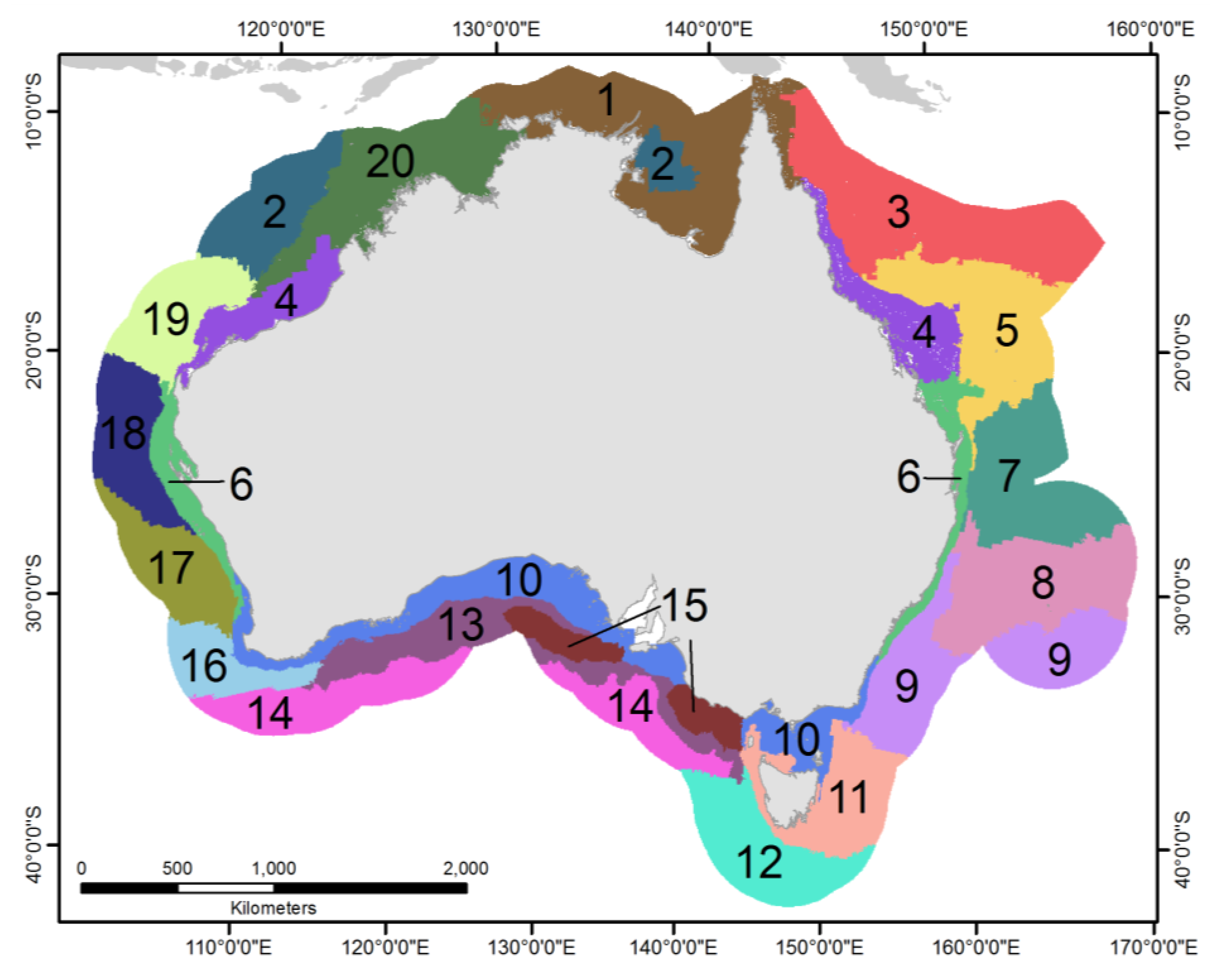
Figure 3.
Box-and-whisker plots of July sound speed profile gradients (in units of (m/s)/m) at selected depths, by zone (x-axes show zone number).
Figure 3.
Box-and-whisker plots of July sound speed profile gradients (in units of (m/s)/m) at selected depths, by zone (x-axes show zone number).
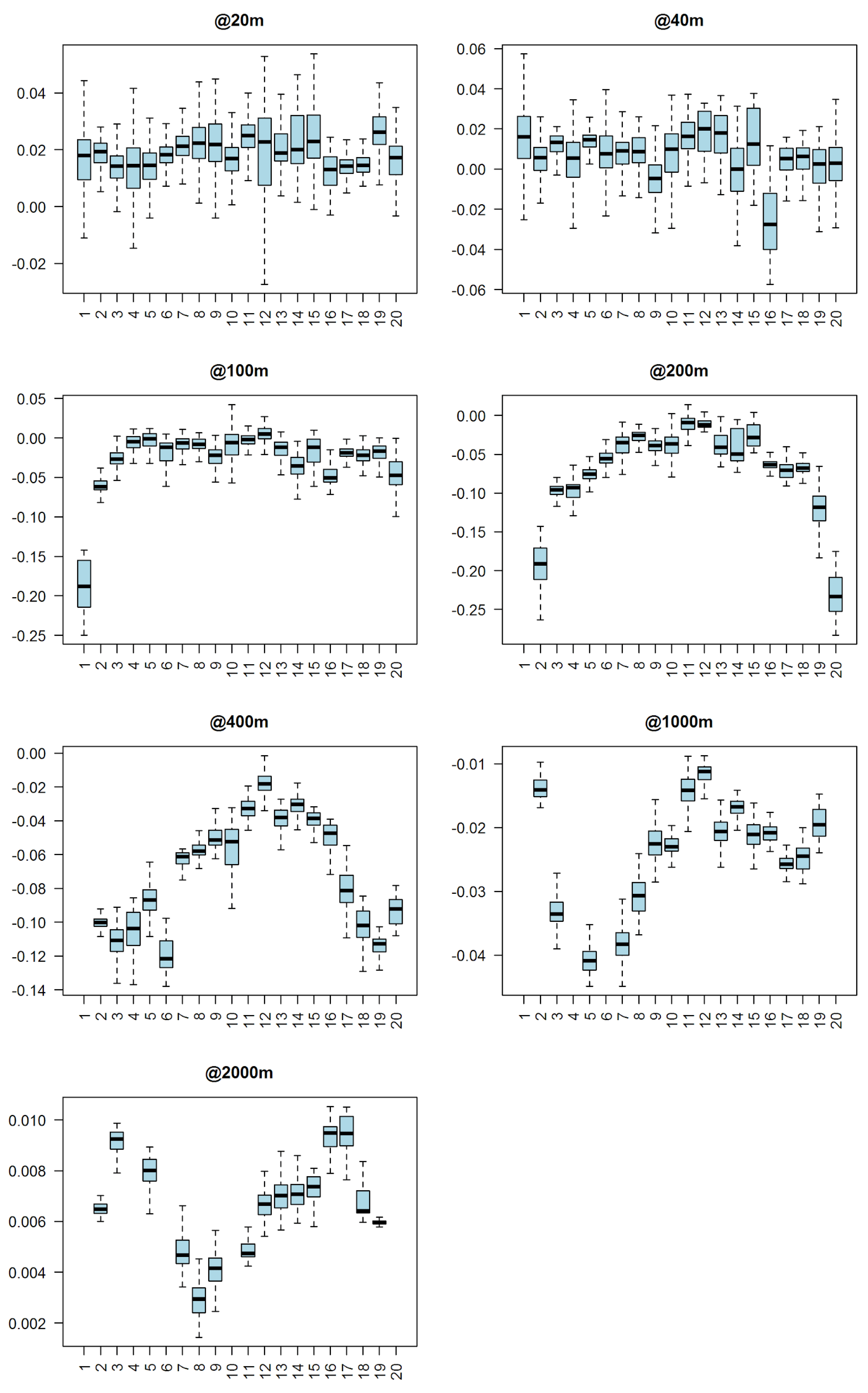
Figure 4.
Box-and-whisker plots of various variables by zone (x-axes show zone number): Sea surface temperature (SST) [kelvin], sea surface salinity [psu], compressional sound speed at the seafloor (Cp) [m/s], shear sound speed at the seafloor (Cs) [m/s], compressional absorption coefficient at the seafloor () [dB/λ], shear absorption coefficient at the seafloor () [dB/λ], density of the top seafloor layer [1000 kg/m3], thickness of the unconsolidated and consolidated sediment [m], water depth [m], and seabed slope [degrees]. Variables used directly in the clustering model are in green boxes.
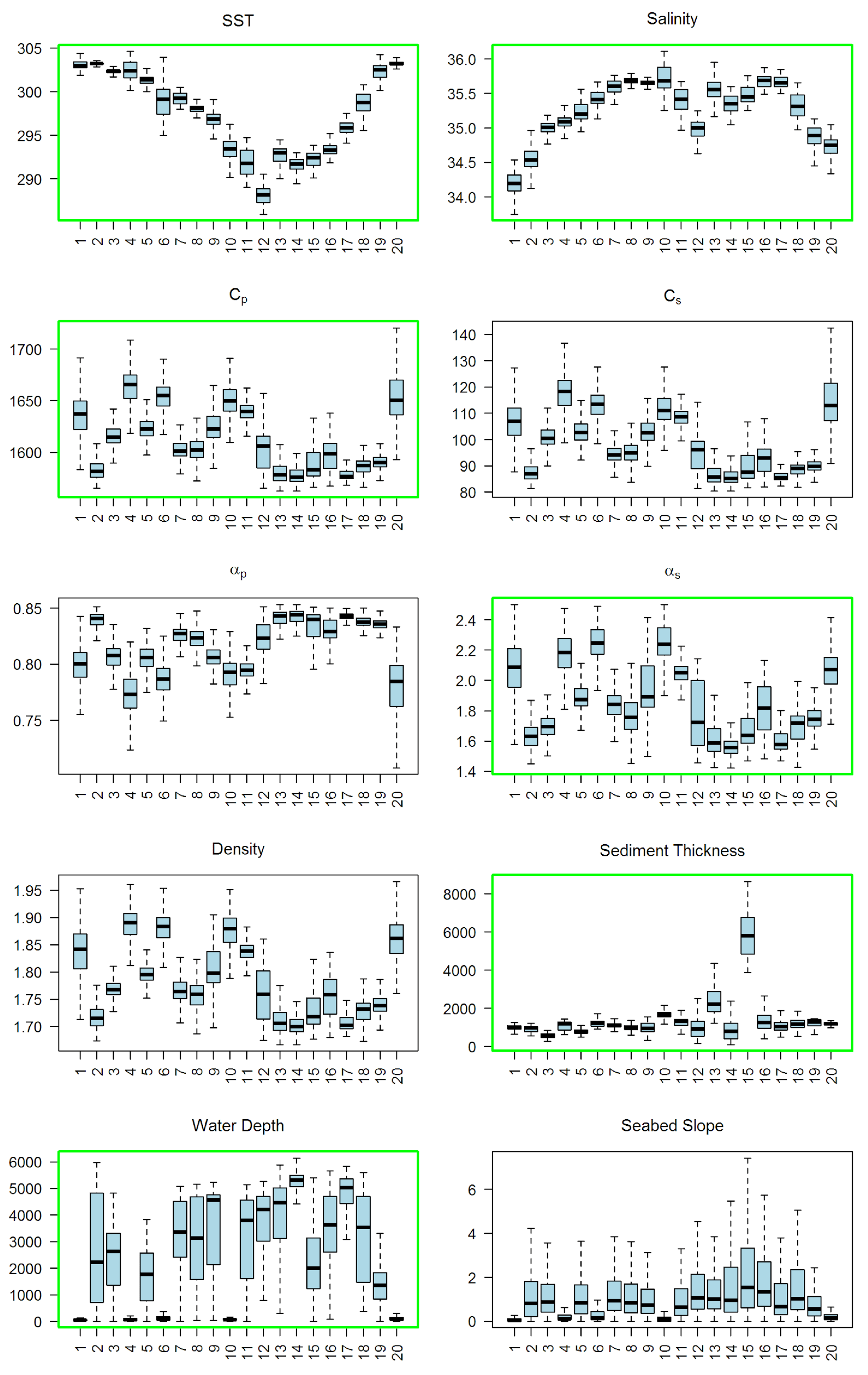
Figure 5.
Maps of selected physical variables with acoustic zones overlaid: Sea surface temperature (SST), sea surface salinity, seafloor %mud, seafloor %sand, sediment thickness, and water depth.
Figure 5.
Maps of selected physical variables with acoustic zones overlaid: Sea surface temperature (SST), sea surface salinity, seafloor %mud, seafloor %sand, sediment thickness, and water depth.

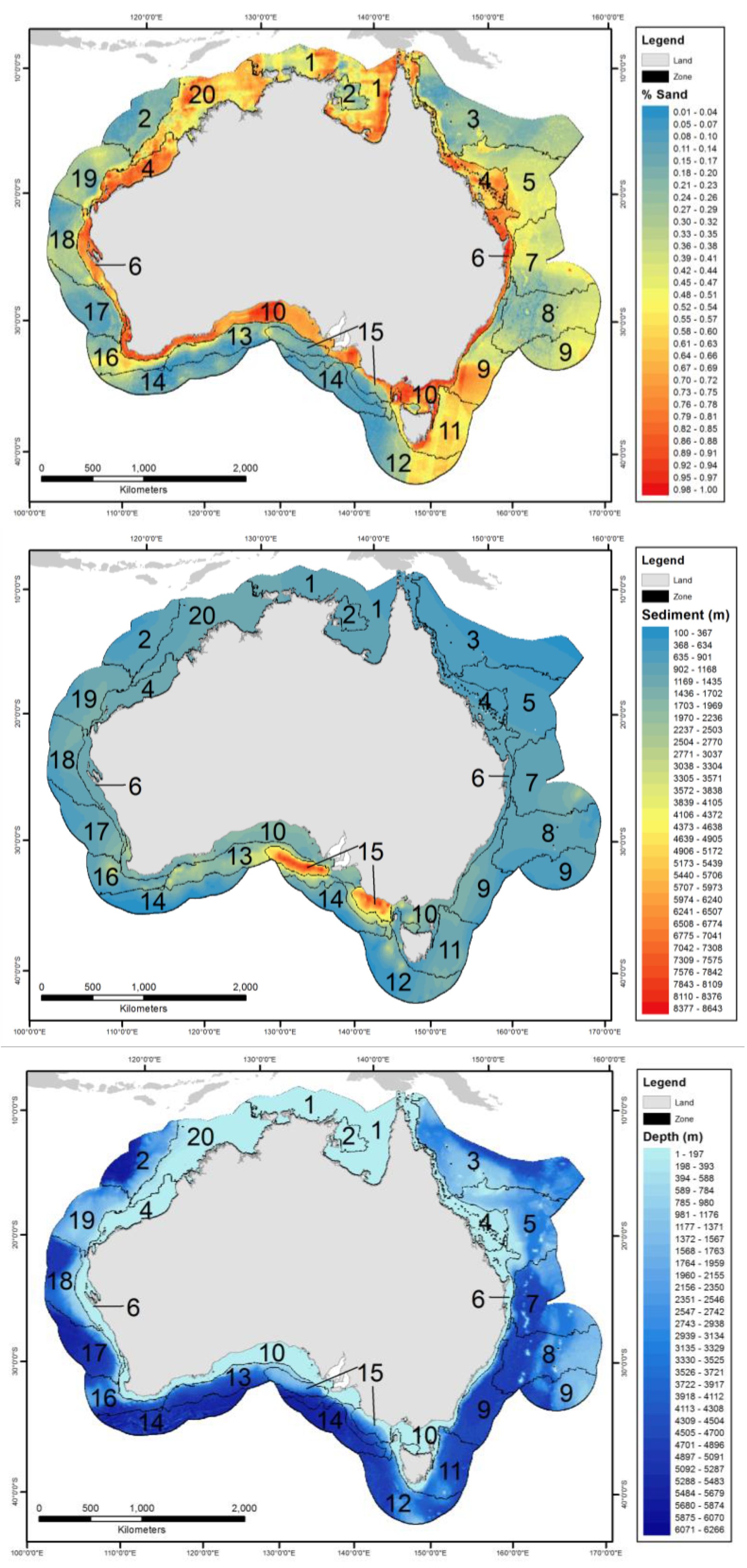
Figure 6.
Sound speed profiles representative of the month of July, coloured by zone. The mean profile for each zone is drawn as a line on top of all profiles within that zone, which are merely shaded.
Figure 6.
Sound speed profiles representative of the month of July, coloured by zone. The mean profile for each zone is drawn as a line on top of all profiles within that zone, which are merely shaded.

Table 1.
List of input and derived variables that affect sound propagation.
| Group Variable | Derived Variable | Input Variable | Source |
|---|---|---|---|
| Water Column | sea surface temperature | sea surface temperature | [6] |
| sea surface salinity | sea surface salinity | [7] | |
| sound speed gradient profile | sound speed profile | [8] | |
| Seafloor | compressional sound speed, shear sound speed, compressional absorption coefficient, shear absorption coefficient, density | % clay | |
| % silt | [11] | ||
| % sand | |||
| % gravel | |||
| sediment thickness | sediment thickness | [13] | |
| bedrock type | bedrock type | [14,15] | |
| Bathymetry | water depth | water depth | [16] |
Table 2.
Interpretation of zones given by the clustering.
| Zone | Name | Description |
|---|---|---|
| 1 | Northern Tropical Shelf | Hot northern zone, shallow water with low salinity. Borders appear to align with salinity change. |
| 2 | Muddy Tropical Shallow | Two areas of northern Australia, one offshore in the West and one in shallow water in the Gulf of Carpentaria. Their predominant features are a muddy seabed, hot temperature, and low salinity. |
| 3 | Eastern Tropical 1 | Excludes coastal waters but spans a range of depths. Separate from neighbouring Zone 5 to the South by water column sound speed profile. Zones 1–3 and 20 have the steepest downward refracting gradients. An abrupt change in salinity defines the border with Zone 1. |
| 4 | Tropical Shelf | Exists on both coasts. Mostly shallow, sandy, coastal water. Hot temperature, medium salinity. |
| 5 | Eastern Tropical 2 | Geoacoustic parameters drive the border with Zone 4, hydroacoustic parameters (i.e., sound speed profiles) drive the borders with Zones 3 and 7. |
| 6 | Sub-Tropical to Temperate Shelf | Exists on both coasts. Warm, shallow, sandy. |
| 7 | Eastern Sub-Tropical Deep | Inner bound at continental shelf. Hydroacoustic parameters drive the separation from Zone 8. |
| 8 | Eastern Temperate Deep 1 | Inner bound at continental shelf. High sea surface salinity. Less downward refracting than Zone 7. |
| 9 | Eastern Temperate Deep 2 | Inner bound at continental shelf. High salinity. Less downward refracting than Zone 8. |
| 10 | Southern Temperate Shelf | Shallow water bounded by the continental slope. High salinity. Sandy seafloor. |
| 11 | Southern Cold | Covers shallow coastal Tasmania but also extends to deep water South-East of Tasmania. Cold water with a strong surface duct in July. |
| 12 | Southern Cold Deep | Most southerly zone. Cold. Less saline surface water than Zone 11. The least sound-focussing sound speed profiles. |
| 13 | Great Australian Bight Temperate Deep 1 | Southern, cold, deep. Inner bound at continental shelf. Shallower yet thicker sediment than Zone 14. |
| 14 | Great Australian Bight Temperate Deep 2 | Southern, cold, deep. |
| 15 | Southern Thick Sediment | An area (2 locations) between Zones 10 and 13 with very high sediment thickness. |
| 16 | Western Temperate Deep 1 | Offshore with a sandy, shallower band resulting in different seabed acoustic properties from neighbouring Zones 14 and 17. Sound speed gradients at 40–1000 m different from neighbouring zones. Inner bound at continental shelf. |
| 17 | Western Temperate Deep 2 | Inner bound at continental shelf. Cooler and more saline than Zone 18 to the North. |
| 18 | Western Sub-Tropical Deep | Offshore, warm. Inner bound at continental shelf. |
| 19 | Western Tropical Offshore | Warm-hot. Downward refracting July profile. Inner bound at continental shelf. Shallower than Zone 2 to the North and Zone 18 to the South. |
| 20 | Western Tropical Shelf | Shallow water. Wide, sandy continental shelf. Hot sea surface; strongly downward refracting. |
Table 3.
Average (±SD) parameters of the 20 acoustic zones produced by the clustering model: Water depth, seafloor slope, sediment thickness, compressional (cp) and shear (cs) speeds, compressional (αp) and shear (αs) absorption coefficients, and density. λ is the acoustic wavelength.
Table 3.
Average (±SD) parameters of the 20 acoustic zones produced by the clustering model: Water depth, seafloor slope, sediment thickness, compressional (cp) and shear (cs) speeds, compressional (αp) and shear (αs) absorption coefficients, and density. λ is the acoustic wavelength.
| Zone | Depth [m] | Slope [Degrees] | Sediment Thickness [m] | Cp [m/s] | Cs [m/s] | αp [dB/λ] | αs [dB/λ] | Density [kg/m3] |
|---|---|---|---|---|---|---|---|---|
| 1 | 51 ± 49 | 0.1 ± 0.5 | 990 ± 139 | 1635 ± 23 | 107 ± 9 | 0.80 ± 0.02 | 2.05 ± 0.18 | 1833 ± 45 |
| 2 | 2583 ± 2047 | 1.5 ± 2.4 | 917 ± 160 | 1584 ± 12 | 88 ± 4 | 0.84 ± 0.01 | 1.65 ± 0.10 | 1720 ± 26 |
| 3 | 2460 ± 1230 | 1.4 ± 1.8 | 580 ± 132 | 1617 ± 13 | 101 ± 5 | 0.81 ± 0.01 | 1.70 ± 0.09 | 1770 ± 24 |
| 4 | 94 ± 131 | 0.4 ± 1.0 | 1076 ± 230 | 1662 ± 23 | 117 ± 10 | 0.78 ± 0.03 | 2.17 ± 0.13 | 1882 ± 37 |
| 5 | 1773 ± 966 | 1.6 ± 2.2 | 764 ± 114 | 1624 ± 13 | 103 ± 5 | 0.80 ± 0.01 | 1.89 ± 0.09 | 1800 ± 23 |
| 6 | 146 ± 200 | 0.5 ± 1.2 | 1225 ± 194 | 1654 ± 16 | 113 ± 7 | 0.79 ± 0.02 | 2.24 ± 0.12 | 1878 ± 29 |
| 7 | 3354 ± 1085 | 1.8 ± 2.7 | 1163 ± 231 | 1603 ± 11 | 95 ± 4 | 0.83 ± 0.01 | 1.83 ± 0.10 | 1765 ± 24 |
| 8 | 3151 ± 1438 | 1.6 ± 2.5 | 976 ± 154 | 1603 ± 13 | 95 ± 5 | 0.82 ± 0.01 | 1.76 ± 0.11 | 1757 ± 26 |
| 9 | 3588 ± 1452 | 1.6 ± 2.6 | 1008 ± 287 | 1623 ± 15 | 102 ± 5 | 0.81 ± 0.01 | 1.93 ± 0.17 | 1803 ± 37 |
| 10 | 126 ± 265 | 0.5 ± 1.9 | 1727 ± 386 | 1650 ± 17 | 112 ± 7 | 0.79 ± 0.02 | 2.25 ± 0.12 | 1874 ± 32 |
| 11 | 3032 ± 1758 | 1.4 ± 2.4 | 1278 ± 316 | 1638 ± 13 | 108 ± 5 | 0.80 ± 0.01 | 2.06 ± 0.11 | 1836 ± 26 |
| 12 | 3821 ± 1057 | 1.9 ± 2.6 | 988 ± 490 | 1603 ± 22 | 95 ± 8 | 0.82 ± 0.02 | 1.77 ± 0.21 | 1758 ± 51 |
| 13 | 3899 ± 1505 | 2.0 ± 3.1 | 2401 ± 730 | 1580 ± 11 | 87 ± 4 | 0.84 ± 0.01 | 1.62 ± 0.12 | 1711 ± 27 |
| 14 | 5240 ± 364 | 2.3 ± 3.5 | 840 ± 498 | 1578 ± 9 | 86 ± 3 | 0.84 ± 0.01 | 1.57 ± 0.08 | 1704 ± 20 |
| 15 | 2157 ± 1413 | 2.6 ± 3.2 | 5848 ± 1120 | 1596 ± 30 | 92 ± 11 | 0.83 ± 0.02 | 1.73 ± 0.24 | 1745 ± 65 |
| 16 | 3616 ± 1252 | 2.5 ± 3.5 | 1339 ± 553 | 1597 ± 14 | 92 ± 5 | 0.83 ± 0.01 | 1.81 ± 0.16 | 1755 ± 36 |
| 17 | 4478 ± 1388 | 1.8 ± 3.4 | 1094 ± 317 | 1579 ± 6 | 86 ± 2 | 0.84 ± 0.00 | 1.60 ± 0.08 | 1708 ± 16 |
| 18 | 3180 ± 1587 | 1.9 ± 2.6 | 1163 ± 225 | 1586 ± 8 | 89 ± 3 | 0.84 ± 0.01 | 1.70 ± 0.10 | 1728 ± 22 |
| 19 | 1515 ± 692 | 1.0 ± 1.1 | 1269 ± 171 | 1591 ± 9 | 90 ± 3 | 0.84 ± 0.01 | 1.75 ± 0.10 | 1740 ± 22 |
| 20 | 135 ± 0134 | 0.3 ± 0.7 | 1200 ± 49 | 1655 ± 28 | 115 ± 12 | 0.78 ± 0.03 | 2.07 ± 0.13 | 1861 ± 40 |
Publisher’s Note: MDPI stays neutral with regard to jurisdictional claims in published maps and institutional affiliations. |
© 2021 by the authors. Licensee MDPI, Basel, Switzerland. This article is an open access article distributed under the terms and conditions of the Creative Commons Attribution (CC BY) license (http://creativecommons.org/licenses/by/4.0/).
Share and Cite
MDPI and ACS Style
Erbe, C.; Peel, D.; Smith, J.N.; Schoeman, R.P. Marine Acoustic Zones of Australia. J. Mar. Sci. Eng. 2021, 9, 340. https://doi.org/10.3390/jmse9030340
AMA Style
Erbe C, Peel D, Smith JN, Schoeman RP. Marine Acoustic Zones of Australia. Journal of Marine Science and Engineering. 2021; 9(3):340. https://doi.org/10.3390/jmse9030340
Chicago/Turabian StyleErbe, Christine, David Peel, Joshua N. Smith, and Renee P. Schoeman. 2021. "Marine Acoustic Zones of Australia" Journal of Marine Science and Engineering 9, no. 3: 340. https://doi.org/10.3390/jmse9030340
Note that from the first issue of 2016, this journal uses article numbers instead of page numbers. See further details here.