Analysis of Typhoon-Induced Waves along Typhoon Tracks in the Western North Pacific Ocean, 1998–2017


1
Marine Science and Technology College, Zhejiang Ocean University, Zhoushan 316000, China
2
Key Laboratory of Space Ocean Remote Sensing and Application, Ministry of Natural Resources, Beijing 100081, China
3
College of Marine Sciences, Shanghai Ocean University, Shanghai 201306, China
*
Author to whom correspondence should be addressed.
J. Mar. Sci. Eng. 2020, 8(7), 521; https://doi.org/10.3390/jmse8070521
Submission received: 30 June 2020
/
Revised: 14 July 2020
/
Accepted: 15 July 2020
/
Published: 16 July 2020
(This article belongs to the Special Issue Storm Tide and Wave Simulations and Assessment)
Abstract
:In this study, Version 5.16 of the WAVEWATCH-III (WW3) model is used to simulate parameters of typhoon-generated wave fields in the Western North Pacific Ocean during the period 1998–2017. From a database of more than 300 typhoons, typhoon tracks are partitioned into six groups by their direction of motion and longitude of recurvature track. For typhoons that recurve east of 140° E, or track toward mainland Asia, regions of high significant wave height (SWH) values are separated by a minimum in SWH near 30° N. Partitioning SWH into wind sea and swell components demonstrates that variations in typhoon tracks produce a much stronger signal in the wind sea component of the wave system. Empirical orthogonal function (EOF) analysis is used to compute the four leading modes of variation in average SWH simulated by the WW3 model. The first EOF mode contributes to 17.3% of the total variance; all other modes contribute less than 10%. The first EOF mode also oscillates on an approximately 1-year cycle during the period 1998–2017. Overall, typhoon-induced wave energy dominates north of 30° N. Temporal analysis of the leading principal component of SWH indicates that (a) the intensity of the wave pattern produced by westward-tracking typhoons decreased during the last 20 years, and (b) typhoons that recurve east of 140° E and those that track westward toward southeast Asia are largely responsible for the decadal variability of typhoon-induced wave distribution.

1. Introduction
Tropical cyclones (TCs) play an important role in water vapor and heat transport at the atmosphere–ocean boundary layer, and typhoon landfall is often accompanied by extreme weather such as damaging winds, torrential rain, storm surge, and breaking waves. These typhoon hazards often cause secondary disasters such as floods, landslides, and mudslides. Among ocean basins, the Western North Pacific (WNP) experiences the highest frequency of TC occurrences worldwide. During the last decade, some studies have evaluated the meteorological factors that influence typhoon tracks in this basin (e.g., [1]) and others have used cluster analysis to study typhoon tracks (e.g., [2]). However, the relationship between meteorological factors that influence typhoon tracks and the distribution of typhoon-induced waves remains understudied, especially from a climate perspective. Therefore, the relationship between typhoon track and the spatial and temporal distribution of typhoon-induced waves merits further exploration.
Traditionally, there are two primary methods to analyze the distribution of the typhoon-induced waves: numerical simulations and satellite remote sensing. Frequently used numerical wave simulations include the wave model (WAM), simulating waves nearshore (SWAN) [3], and WAVEWATCH-III (WW3) [4]. The WW3 model has been widely used for wave simulation in many oceanic regions, including the Pacific Ocean [5,6], Indian Ocean [7], China Seas [8,9], and North Atlantic Ocean [10,11]. The WW3 model has been demonstrated to be suitable for studying typhoon-induced waves through validation against moored buoys and satellite altimeter measurements [12,13,14]. Moreover, the WW3 model is capable of simulating long-period waves for the wave climate analysis [11,15]. Satellite data used for real-time wave observations include altimeter data [16] and synthetic aperture radar (SAR) data [17]. Spaceborne SARs, such as the Chinese Gaofen-3 SAR, feature a large swath width (>500 km) and fine spatial resolution (e.g., 150 m), thereby enabling high-resolution monitoring of typhoon winds [17,18,19] and waves [20,21,22,23] on large spatial scales. However, SAR data are only acquired on demand and are therefore unavailable for long-term studies.
Numerical wave models such as WAM, SWAN, and WW3 are widely used for long-term wave climate analysis under various oceanic and atmospheric conditions [24,25,26,27]. These models have been used to analyze the wave climate of the open ocean, coastal regions, and inland seas, including studies in the North Atlantic [27], the Bohai Sea [26], the Yellow Sea [25], the East China Sea [24], and the Black Sea [28]. These numerical wave models have also been used to study the climate of extreme waves [29], including in specific regions such as the China Seas [30], the East China Sea [31], and the Mediterranean Sea [32].
Aspects of numerical wave simulation work focus on evaluating wave climatology in future climates affected by sea-level rise [33] and changes in sea-surface temperatures [34]. Some of these studies have included TC events; for example, Niroomandi et al. (2018) used SWAN to evaluate the wave climate of the Chesapeake Bay, including four TCs or ex-TCs that affected the Bay between 2008 and 2012 [35]. That study, however, analyzed a limited region and a small number of TCs. Therefore, a targeted study of typhoon-induced waves in the WNP is necessary to provide information about the long-term extreme wave climate and the typhoon-induced wave fields produced by various typhoon tracks over the WNP.
In this study, we use the WW3 model to simulate the 1998–2017 Western North Pacific typhoon-induced wave climate. We analyze the wave climate patterns produced by varying typhoon track groups during this period. The remainder of this paper is organized as follows: the setup of the WW3 model is described in Section 2; typhoon track classification and wave analysis corresponding to each track type are described in Section 3. Besides, EOF analysis of significant wave height patterns is also presented; the natural variability of twenty-years’ variability in typhoon-induced wave distribution is exhibited in Section 4; and the conclusions are summarized in Section 5.
2. Materials and Methods
We used the WW3 model to simulate typhoon-induced wave parameters (significant wave height (SWH), mean wave period (MWP), and mean wave length (MWL)) in the WNP during the 20-year period 1998–2017. The simulated area is a rectangle from 5° S to 65° N and 93° E to 167° W; bathymetry is provided by the general bathymetry chart of the oceans (GEBCO) at 0.1° horizontal resolution (Figure 1). Data from six National Data Buoy Center (NDBC) buoys in the Western North Pacific Ocean are used to validate the WW3-simulated SWHs. Locations of the NDBC buoys are marked Figure 1. Typhoon track data are provided by the Regional Specialized Meteorological Centre (RSMC) Tokyo-Typhoon Center of the Japan Meteorological Agency (JMA). Typhoons that lasted more than five days were included in this study, yielding over 300 tracks during the 1998–2017 period (Figure 1).
The WW3 model was developed by the National Centers for Environmental Prediction of the National Oceanic and Atmospheric Administration (NOAA NCEP). The WW3 model has been shown to perform well at simulating the characteristics of TC-induced waves [36,37]. In this study, 0.125° gridded ECMWF wind data provide forcing for WW3. Bathymetry data for the WW3 simulation were obtained at 0.1° horizontal resolution from GEBCO [38]. The resolution of the bathymetry data was 0.5°. The model was initialized at 00:00 UTC 1 January 1998 and terminated at 00:00 UTC 1 January 2018. Wave data were output at 0.5° spatial resolution and 30 min temporal resolution. Data from the six NDBC buoys allowed us to verify the WW3 results against more than three million observations during the simulation period. Figure 2 shows that the WW3-simulated results were close to the measurements from NDBC buoys (>300,000), showing a 0.43 m root mean square error (RMSE) with a 0.94 correlation (COR). The results indicate the reliability of the model.
3. Results
3.1. Classification of Typhoon Tracks
In the WNP, most typhoons either recurve or move approximately linearly, while just a few storms follow complex tracks such as loops. In this study, we only included typhoon tracks with durations of more than five days and omitted the small number of complex tracks. Using the track data, we clustered typhoon tracks according to genesis and extinction locations. If the genesis location is at the maximum longitude (farthest east) anywhere on the TC track, and the extinction location is at the minimum longitude (farthest west), the track is assigned to the Northeast Shift group. If the genesis location is located at the maximum longitude anywhere in the track (farthest east), and extinction location is at the minimum longitude (farthest west), the track is assigned to the straight-moving group. Within the straight-moving group, the average slope k of tropical cyclone track calculating between the genesis and extinction locations was used to further partition tracks. If the arctangent of k was between 7π/8 and 9π/8, the track was assigned to the west shift group. If the arctangent of k was between 5π/8 and 7π/8, the track was assigned to the northwest shift group [1,2,39]. If neither the genesis location nor the extinction location was located at the minimum longitude, the track belonged to the recurve group. Members of the recurve group were further partitioned by their westernmost location, known as the recurve point. If the longitude of the recurve point was >140°, the track was assigned to the east turn group. If the longitude of the recurve point <125°, the track was assigned to the west turn group. If the longitude of the recurve point was between 125 and 140°, the track was assigned to the middle turn group [40]. Thus, all typhoon tracks with duration >5 days were assigned to one of six track groups: northeast shift, east turn, middle turn, west turn, northwest shift, and west shift. The middle turn group was the most populous track group (n = 91), whereas the northeast shift was the least populous (n = 28; Figure 3).
3.2. Parameters of Typhoon-Induced Waves
In order to remove the background wave parameters without typhoons, we chose the wave parameters simulation result during the period of each typhoon path group. Figure 4 shows the average WW3-simulated SWHs from each typhoon path group, in which the black polylines represent the typical path in each path group. Maximum SWH (MS) values were at similar locations for all typhoon path groups: between 50° N–60° N and 160° E–187° W at the end of the typhoon’s lifecycle. Furthermore, the asymmetrical structure was found to the right and left of the typhoon tracks. It was not surprising that this SWH pattern followed the tracks of the northeast shift, east turn, and middle turn groups (Figure 4a–c corresponding to Figure 3a–c), because no land barriers occurred in those regions to interrupt the wave pattern. In the more westward typhoon track groups (Figure 3d–f), two relatively high SWH regions were observed around 30° N (Figure 4c–f). In particular, the second SWH peak moved from the East China Sea to the South China Sea as typhoon tracks shifted more westward. Since West Shift typhoon tracks remained far from the northerly-located Monsoon region, waves in that area are determined by weather systems in other regions, such as the monsoon wind and the Westerly Belt wind at the northern Central Pacific Ocean [41]. The average mean wave period for each typhoon path group is shown in Figure 5; MWP patterns were also consistent with the typhoon track groups, especially for the northeast shift (Figure 5a) and northwest shift (Figure 5e) groups. The MWP peak area was located in the Japan Eastern Ocean in Figure 5a and the East China Sea in Figure 5e. However, maps of the average mean wave length (Figure 6) did not show this pattern. Taking the results together, the typhoon track appeared to substantially influence the basin-scale typhoon-induced wave distribution.
To further study the relationship between typhoon track and SWH distribution, we partitioned SWH values into individual wind sea and swell components by the WW3 model output. Figure 7 and Figure 8 show the average wind sea and swell components, respectively, of simulated SWH for each typhoon track group. The wind sea SWH component reached maximum values of approximately 3 m near the typhoon tracks, while the swell SWH component reached values up to 2 m. Although the waves produced by other weather systems blur the signal of typhoon-induced waves at latitudes above 50° N, it is clear from Figure 7d–f that the wind sea SWH component varied coherently between the track groups. The maximum wind-sea SWH was on the typhoon path, such as the middle turn (Figure 7c), west turn (Figure 7d), and northwest shift (Figure 7e). However, no consistent relationship was observed between the swell SWH component and typhoon tracks. We therefore concluded that variations in typhoon track between the typhoon track groups primarily affected the distribution of SWH through the wind sea component of the wave system.
3.3. Analysis of the Leading EOF Modes of Significant Wave Height Variation
As for the EOF analysis for the SWH data on the typhoon path period, we did not find the consequent EOF modes result and the time series result remained interceptive. Thus, to study the spatial and temporal distribution of typhoon-induced SWH in the 1998–2017 period, empirical orthogonal function (EOF) analysis of average SWH was performed. EOF analysis decomposed the dataset into a series of orthogonal functions. The eigenvalue error method proposed by North et al. (1982) was applied to test the significance of the EOF outputs [42]. The range of eigenvalue error was calculated by the following equation.
in which, ej is the eigenvalues error, λj is the eigenvalue, and n is the sample number. The judgment equation is stated as:
If the Equation (2) is derived, the two eigenvalues representing the modes of EOF is reliable.
As shown the Table 1, we found the four leading EOF modes of average SWH passed the significance test. The leading EOFs indicate the patterns that explain the greatest variation within the dataset.
The spatial distributions of the four leading EOF modes of average SWH are shown in Figure 9. From the EOF patterns we computed two principal component variables: PC(t), which represents the amplitude of the EOF pattern at a single time, and PC(max), which represents the maximum EOF pattern amplitude during the 1998–2017 period. The first EOF mode (Figure 9a) contributes 17.3% of the total variance in average SWH. It represents a dipole in average SWH between the central North Pacific and the Western Pacific near Japan. This indicates that the typhoon-induced wave energy dominated near Japan, as well as in the Sea of Japan and the East China Sea. The second mode (Figure 9b) contributed to 8.4% of the total variance. This EOF shows a tripole pattern, with elevated SWH values south of Japan and Korea associated with depressed values south of the Kamchatka Peninsula, and elevated values near the Aleutian Islands. The third (Figure 9c) and fourth (Figure 9d) EOF modes contributed to 8.4% and 7.0% of the total variance, respectively. The corresponding time series of PC(t)/PC(max) are presented in Figure 10, in which the values were normalized into a range between −0.5 and 0.5. The amplitude of PC(t)/PC(max) was clearly larger for the first EOF mode (Figure 10a) than for the other three modes. The first EOF mode oscillates on a roughly 1-year cycle, varying between approximately 0.4 and −0.5. This behavior indicates an interannual variability pattern in typhoon-induced SWH distribution over the Western North Pacific. For the second through fourth EOF modes (Figure 10b–d), the time series of PC(t)/PC(max) show no clear cyclical trends.
4. Discussion
As for the EOF modes result (Figure 9), we found the EOF modes distribution in the East China Sea was not completely consistent with the result in Wang et al. (2016) [43]. Although a similar magnitude was achieved in the first mode, the big rate was located in the North East China Sea and the trend of EOF, which is different from the result in [43]. There was a high wave in the Japan Sea caused by the strong seasonal northerly wind. In the Pacific Ocean, summer monsoon seasonal wind (south westerly) and typhoons may cause a high sea state. Such seasonality was derived by the EOF analysis in Figure 9a and this behavior is also proposed in [43]. In the second and third modes, there was no consistency with two analyses. As for the corresponding time series of PC(t)/PC(max) (Figure 10), our analysis had a similar trend of the time period result in [35,43].
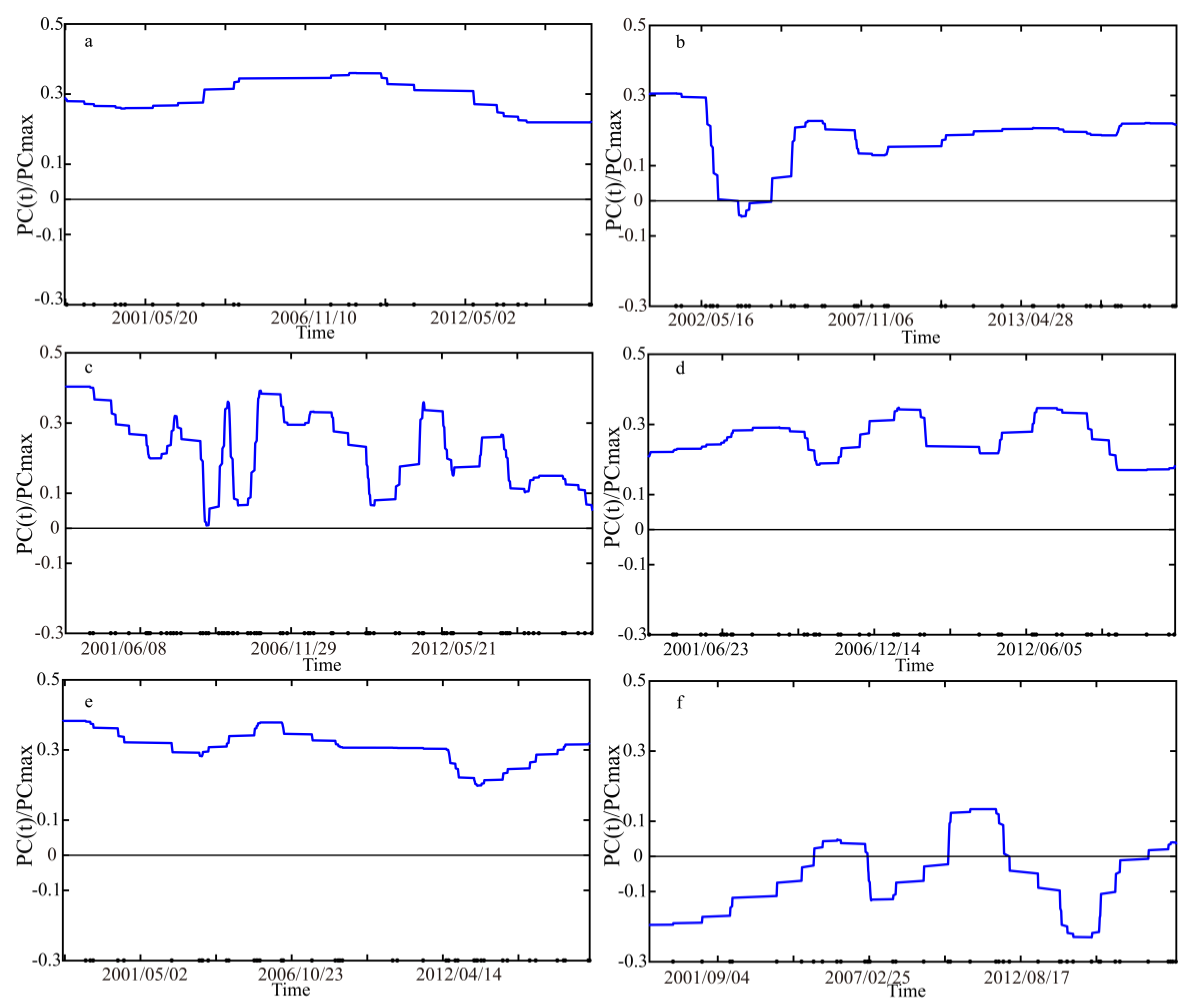
Here, we analyzed the interannual variability of PC(t)/PC(max) for all typhoons from 1998 to 2017. Figure 11 shows the values of PC(t)/PC(max) of the first EOF for each typhoon track group. Overall, PC(t)/PC(max) values were positive, indicating that typhoons tended to produce higher SWH values near Japan and in nearby seas, and lower values over the central North Pacific (Figure 9a). However, in the West Shift group (Figure 11f), the PC(t)/PC(max) values generally decreased in amplitude, indicating a weakening signal from westward-tracking typhoons during the 20-year period studied. In the northeast shift (Figure 11a), west turn (Figure 11d), and northwest shift groups, the PC(t)/PC(max) values remained relatively constant, indicating that no climate trend in the typhoon-induced waves pattern could be detected from 1998 to 2017. In the east turn (Figure 11b) and middle turn (Figure 11c) track groups, PC(t)/PC(max) values fluctuated substantially during the 1998–2017 period. Indeed, it is better to study the change in the climate of typhoon-induced wave distribution with a minimum 30-year period. Nevertheless, we presumed that this short-term behavior might reflect possible changes in the climate of typhoon-induced wave distribution.
5. Conclusions
The climate of tropical cyclone-induced waves remains an understudied topic in the oceanography community. In this study, we analyzed the wave distribution from typhoons in the Western North Pacific Ocean during the period 1998–2017. Typhoon tracks were partitioned into six groups based on track direction and longitude of recurvature. The WAVEWATCH-III Model (WW3; Version 5.16) was used to simulate waves over the Western North Pacific from 1998 to 2017. Simulated wave parameters (significant wave height (SWH), mean wave period (MWP), and mean wave length (MWL)) associated with each typhoon track group were analyzed. Simulation results revealed that the typhoon track substantially affected typhoon-induced wave distribution, especially for SWH and MWP. Across the track groups, elevated SWH values tended to occur in a symmetrical structure cantered on the typhoon path. Typhoons that recurved between 125° E and 140° E, or west of 140° E, produced a region of elevated SWH values south and southwest of the Japanese main islands, respectively, with minimum SWH values near 30° N. In the farther westward typhoon track groups (west turn, northwest shift, and west shift), two relatively high SWH regions were observed around 30° N. In particular, the secondary peak of SWH moved from the East China Sea to the South China Sea when typhoon tracks shifted farther westward. Furthermore, partitioning simulated SWH into wind sea and swell components indicates that typhoon track differences primarily contributed to differences in the wind sea component of SWH.
Empirical orthogonal function (EOF) analysis was used to evaluate the main modes of SWH variation across the set of simulated typhoon-induced waves. The first mode contributed to 17.3% of the total variance, with other modes contributing less than 10%. The first EOF mode was associated with a dipole of SWH values, with opposite values near Japan and in the central North Pacific.
The time evolution of the principal component (PC) of EOF 1 for each typhoon track group, relative to the maximum PC value during 1998–2017, was calculated to further study the climate of WW3-simulated SWH for each type of typhoon path. The first EOF mode revealed that the SWH pattern oscillated on an approximately 1-year cycle and thus appeared to show possible short-term climate signals within the 1998–2017 period, while other EOF modes had no clear cyclical trends. Typhoons that recurved east of 140° E, and those that tracked westward toward Southeast Asia, oscillated substantially during the period, and thus appeared to show short-term natural variability signals within the 1998–2017 period. In the near future, we planned to perform more analyses about the simulated waves using the WW3 model under the background of typhoons, which remove the basic characteristics of ocean waves in the Northwestern Pacific.
Author Contributions
W.S., Y.W. and J.Z. came up the original idea and designed the experiments. Y.H. and J.Z. contribute to wave simulations from the WW3 model. W.S. and Y.H. analyzed the dataset. Y.W. and J.Z. provided great help for the data analysis and discussions. All authors contributed to the writing and revising of the manuscript. All authors have read and agreed to the published version of the manuscript.
Funding
This research was funded by the National Key Research and Development Program of China, grant number 2017YFA0604901, National Natural Science Foundation of China, grant number 41806005, 41776183 and 41976174, Public Welfare Technical Applied Research Project of Zhejiang Province of China, grant number LGF19D060003 and Science and Technology Project of Zhoushan City of China, grant number 2019C21008.
Acknowledgments
We appreciate the National Centers for Environmental Prediction (NCEP) of the National Oceanic and Atmospheric Administration (NOAA) for providing the source code for the WAVEWATCH-III (WW3) model. The European Centre for Medium-Range Weather Forecasts (ECMWF) wind data were accessed via http://www.ecmwf.int. The General Bathymetry Chart of the Oceans (GEBCO) data were downloaded via ftp.edcftp.cr.usgs.gov. The National Data Buoy Center (NDBC) provided buoy data via http://www.ndbc.noaa.gov/. Typhoon parameters were provided by the Japan Meteorological Agency (JMA) via http://www.jma.go.jp.
Conflicts of Interest
The authors declare no conflict of interest.
References
- Yuan, J.P.; Jiang, J. The relationships between tropical cyclone tracks and local SST over the western north pacific. J. Trop. Meteorol. 2011, 17, 120–127. [Google Scholar]
- Kim, H.K.; Seo, K.H. Cluster analysis of tropical cyclone tracks over the western north pacific using a self-organizing map. J. Clim. 2016, 29, 3731–3750. [Google Scholar] [CrossRef]
- Akpınar, A.; Vledder, G.P.V.; Kömürcü, M.İ.; Özger, M. Evaluation of the numerical wave model (SWAN) for wave simulation in the Black Sea. Cont. Shelf Res. 2012, 50, 80–99. [Google Scholar] [CrossRef]
- Kim, T.R.; Lee, J.H. Comparison of high wave hindcasts during Typhoon Bolaven (1215) using SWAN and WAVEWATCH III model. J. Coast. Res. 2018, 85, 1096–1100. [Google Scholar] [CrossRef]
- Bi, F.; Song, J.B.; Wu, K.J.; Xu, Y. Evaluation of the simulation capability of the Wavewatch III model for Pacific Ocean wave. Acta Oceanol. Sin. 2015, 34, 43–57. [Google Scholar] [CrossRef]
- Zheng, K.W.; Sun, J.; Guan, C.L.; Shao, W.Z. Analysis of the global swell and wind sea energy distribution using WAVEWATCH III. Adv. Meteorol. 2016, 2016, 8419580. [Google Scholar] [CrossRef] [Green Version]
- Shukla, R.P.; Kinter, J.L.; Shin, C.S. Sub-seasonal prediction of significant wave heights over the Western Pacific and Indian Oceans, part II: The impact of ENSO and MJO. Ocean Model. 2018, 123, 1–15. [Google Scholar] [CrossRef]
- He, H.L.; Xu, Y. Wind-wave hindcast in the Yellow Sea and the Bohai Sea from the year 1988 to 2002. Acta Oceanol. Sin. 2016, 35, 46–53. [Google Scholar] [CrossRef]
- Zheng, K.W.; Osinowo, A.A.; Sun, J.; Hu, W. Long-term characterization of sea conditions in the East China Sea using significant wave height and wind speed. J. Ocean Univ. China 2018, 17, 733–743. [Google Scholar] [CrossRef]
- Gallagher, S.; Tiron, R.; Dias, F. A long-term nearshore wave hindcast for Ireland: Atlantic and Irish Sea coasts (1979–2012). Ocean Dyn. 2014, 64, 1163–1180. [Google Scholar] [CrossRef]
- Guo, L.L.; Perrie, W.; Long, Z.X.; Toulany, B.; Sheng, J.Y. The impacts of climate change on the autumn North Atlantic wave climate. Atmosphere-Ocean 2015, 53, 491–509. [Google Scholar] [CrossRef]
- Shao, W.Z.; Sheng, Y.X.; Li, H.; Shi, J.; Ji, Q.Y.; Tai, W.; Zuo, J.C. Analysis of wave distribution simulated by WAVEWATCH-III model in typhoons passing Beibu Gulf, China. Atmosphere 2018, 8, 265. [Google Scholar] [CrossRef] [Green Version]
- Sheng, Y.X.; Shao, W.Z.; Li, S.Q.; Zhang, Y.M.; Yang, H.W.; Zuo, J.C. Evaluation of typhoon waves simulated by WaveWatch-III model in shallow waters around Zhoushan islands. J. Ocean Univ. China 2019, 19, 365–375. [Google Scholar] [CrossRef]
- Fan, Y.; Lin, S.J.; Held, I.M.; Yu, Z.; Tolman, H.L. Global ocean surface wave simulation using a coupled atmosphere-wave model. J. Clim. 2012, 25, 6233–6252. [Google Scholar] [CrossRef]
- Gallagher, S.; Gleeson, E.; Tiron, R.; Mcgrath, R.; Dias, F. Wave climate projections for Ireland for the end of the 21st century including analysis of EC-Earth winds over the North Atlantic Ocean. Int. J. Clim. 2016, 36, 4592–4607. [Google Scholar] [CrossRef]
- Li, S.Q.; Guan, S.D.; Hou, Y.J.; Liu, Y.H.; Bi, F. Evaluation and adjustment of altimeter measurement and numerical hindcast in wave height trend estimation in China’s coastal seas. Int. J. Appl. Earth Obs. Geoinf. 2018, 67, 161–172. [Google Scholar] [CrossRef]
- Li, X.F. The first Sentinel-1 SAR image of a typhoon. Acta Oceanol. Sin. 2015, 34, 1–2. [Google Scholar] [CrossRef]
- Li, X.F.; Zhang, J.A.; Yang, X.F.; Pichel, W.G.; DeMaria, M.; Long, D.; Li, Z.W. Tropical cyclone morphology from spaceborne synthetic aperture radar. Bull. Am. Meteorol. Soc. 2013, 94, 215–230. [Google Scholar] [CrossRef] [Green Version]
- Ji, Q.Y.; Shao, W.Z.; Sheng, Y.X.; Yuan, X.Z.; Sun, J.; Zhou, W.; Zuo, J.C. A promising method of cyclone wave retrieval from Gaofen-3 synthetic aperture radar image in VV-polarization. Sensors 2018, 18, 2064. [Google Scholar] [CrossRef] [PubMed] [Green Version]
- Romeiser, R.; Graber, H.C.; Caruso, M.J.; Jensen, R.E.; Walker, D.T.; Cox, A.T. A new approach to ocean wave parameter estimates from C-band ScanSAR images. IEEE Trans. Geosci. Remote Sens. 2015, 53, 1320–1345. [Google Scholar] [CrossRef]
- Shao, W.Z.; Li, X.F.; Hwang, P.A.; Zhang, B.; Yang, X.F. Bridging the gap between cyclone wind and wave by C-band SAR measurements. J. Geophys. Res. Oceans 2017, 122, 6714–6724. [Google Scholar] [CrossRef]
- Shao, W.Z.; Hu, Y.Y.; Yang, J.S.; Nunziata, F.; Sun, J.; Li, H.; Zuo, J.C. An empirical algorithm to retrieve significant wave height from Sentinel-1 synthetic aperture radar imagery collected under cyclonic conditions. Remote Sens. 2018, 10, 1367. [Google Scholar] [CrossRef] [Green Version]
- Ding, Y.Y.; Zuo, J.C.; Shao, W.Z.; Shi, J.; Yuan, X.Z.; Sun, J.; Hu, J.C.; Li, X.F. Wave parameters retrieval for dual-polarization C-band synthetic aperture radar using a theoretical-based algorithm under cyclonic conditions. Acta Oceanol. Sin. 2019, 38, 21–31. [Google Scholar] [CrossRef]
- Chen, Y.P.; Xie, D.M.; Zhang, C.K.; Qian, X.S. Estimation of long-term wave statistics in the East China Sea. J. Coast. Res. 2013, 65, 177–182. [Google Scholar] [CrossRef]
- Hwang, P.A.; Bratos, S.M.; Teague, W.J.; Wang, D.W.; Jacobs, G.A.; Resio, D.T. Winds and waves in the yellow and east China seas: A comparison of space-borne altimeter measurements and model results. J. Oceanogr. 1999, 55, 307–325. [Google Scholar] [CrossRef]
- Liang, B.C.; Liu, X.; Li, H.J.; Wu, Y.J.; Lee, D.Y. Wave Climate Hindcasts for the Bohai Sea, Yellow Sea, and East China Sea. J. Coast. Res. 2014, 32, 172–180. [Google Scholar]
- Markina, M.Y.; Gavrikov, A.V. Wave climate variability in the North Atlantic in recent decades in the winter period using numerical modeling. Oceanology 2016, 56, 320–325. [Google Scholar] [CrossRef]
- Divinsky, B.V.; Kosyan, R.D. Spatiotemporal variability of the Black Sea wave climate in the last 37 years. Cont. Shelf Res. 2017, 136, 1–19. [Google Scholar] [CrossRef]
- Caires, S.; Swail, V.R.; Wang, X.L.L. Projection and Analysis of Extreme Wave Climate. J. Clim. 2006, 19, 5581–5605. [Google Scholar] [CrossRef]
- Li, J.X.; Chen, Y.Q.; Pan, S.Q. Modelling of Extreme Wave Climate in China Seas. J. Coast. Res. 2016, 75, 522–526. [Google Scholar] [CrossRef] [Green Version]
- He, H.L.; Song, J.B.; Bai, Y.F.; Xu, Y.; Wang, J.J.; Bi, F. Climate and extrema of ocean waves in the East China Sea. Sci. China Earth Sci. 2018, 7, 1–15. [Google Scholar] [CrossRef]
- Sartini, L.; Mentaschi, L.; Besio, G. Comparing different extreme wave analysis models for wave climate assessment along the Italian coast. Coast. Eng. 2015, 100, 37–47. [Google Scholar] [CrossRef]
- Suursaar, Ü.; Kullas, T. Decadal changes in wave climate and sea level regime: The main causes of the recent intensification of coastal geomorphic processes along the coasts of Western Estonia? WIT Trans. Ecol. Environ. 2009, 126, 105–116. [Google Scholar]
- Shimura, T.; Mori, N.; Mase, H. Future Projection of Ocean Wave Climate: Analysis of SST Impacts on Wave Climate Changes in the Western North Pacific. J. Clim. 2015, 28, 3171–3190. [Google Scholar] [CrossRef] [Green Version]
- Niroomandi, A.; Maa, G.F.; Ye, X.Y.; Lou, S.; Xue, P.F. Extreme value analysis of wave climate in Chesapeake Bay. Ocean Eng. 2018, 159, 22–36. [Google Scholar] [CrossRef]
- Liu, Q.X.; Babanin, A.; Fan, Y.L.; Zieger, S.; Guan, C.L.; Moon, I.J. Numerical simulations of ocean surface waves under hurricane conditions: Assessment of existing model performance. Ocean Model. 2017, 118, 73–93. [Google Scholar] [CrossRef]
- Zieger, S.; Babanin, A.V.; Rogers, W.E.; Young, I.R. Observation-based source terms in the third-generation wave model WAVEWATCH. Ocean Model. 2015, 96, 2–25. [Google Scholar] [CrossRef] [Green Version]
- Weatherall, P.; Marks, K.M.; Jakobsson, M.; Schmitt, T.; Tani, S.; Arndt, J.E.; Rovere, M.; Chayes, D.; Ferrini, V.; Wigley, R. A new digital bathymetric model of the world’s oceans. Earth Space Sci. 2015, 2, 331–345. [Google Scholar] [CrossRef]
- Nakamura, J.; Lall, U.; Kushnir, Y.; Camargo, S.J. Classifying North Atlantic Tropical Cyclone Tracks by Mass Moments. J. Clim. 2009, 22, 5481–5494. [Google Scholar] [CrossRef]
- Yin, H.; Wang, Y.Q.; Zhong, W. Characteristics and influence factors of the rapid intensification of tropical cyclone with different tracks in Northwest Pacific. J. Meteorol. Sci. 2016, 36, 194–203. (In Chinese) [Google Scholar]
- Zhu, Z.X.; Zhou, K. Simulation and Analysis of Ocean Wave in the Northwest Pacific Ocean. Appl. Mech. Mater. 2012, 212, 430–435. [Google Scholar] [CrossRef]
- North, G.R.; Bell, T.L.; Cahalan, R.F.; Moeng, F.J. Sampling Errors in the Estimation of Empirical Orthogonal Functions. Mon. Weather Rev. 1982, 110, 699. [Google Scholar] [CrossRef]
- Wang, J.; Dong, C.M.; He, Y.J. Wave climatological analysis in the East China Sea. Cont. Shelf Res. 2016, 120, 26–40. [Google Scholar] [CrossRef]
Figure 1.
Bathymetric topography of the North West Pacific Ocean with high spatial resolution at a 0.1° grid in the area between 5° S and 65° N, 93° and 193° E. The color indicates the bathymetric topography. The red triangle indicates the locations of the National Data Buoy Center (NDBC) buoys. The black lines represent the typhoon track from Japan Meteorological Agency (JMA).
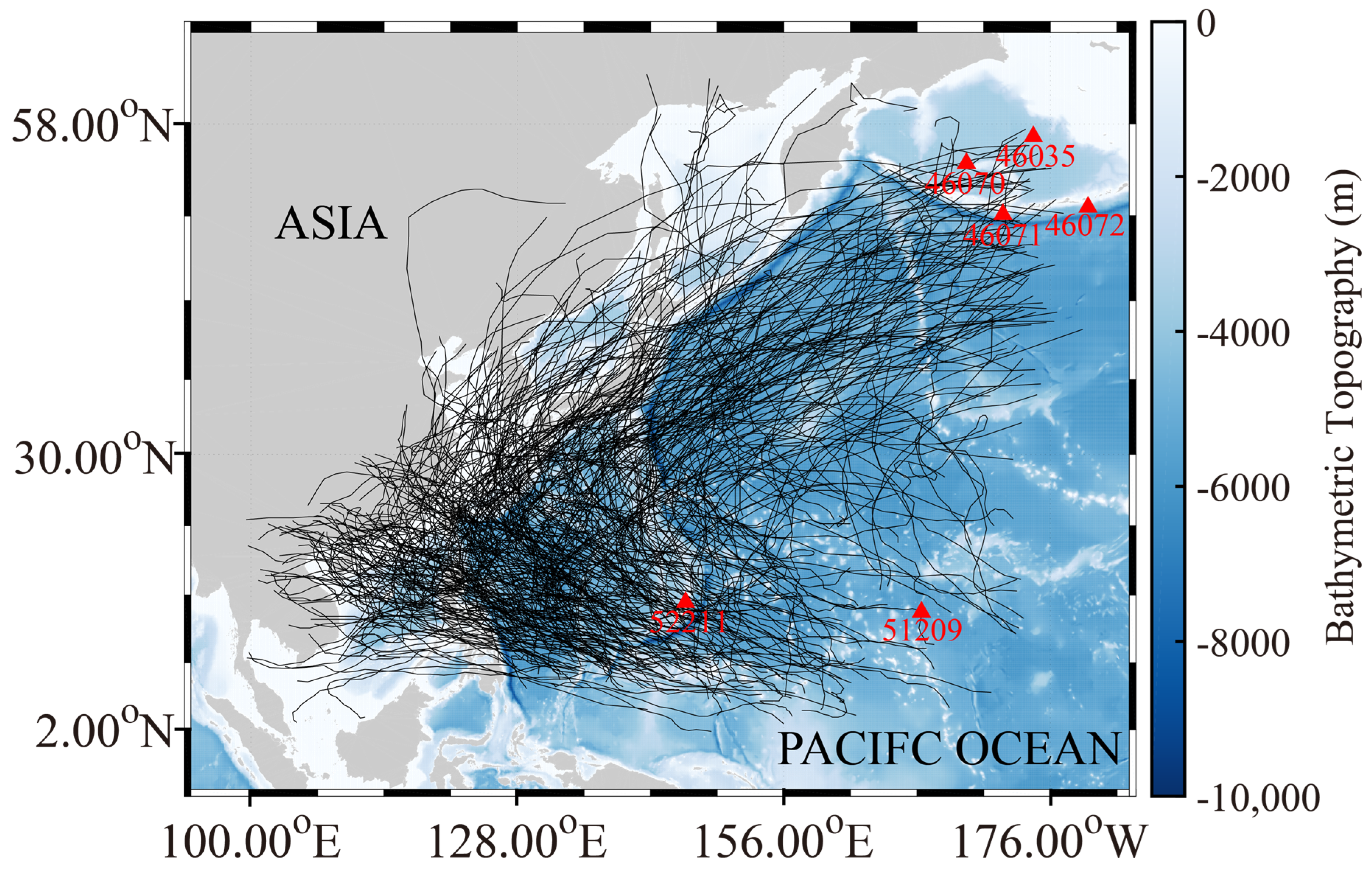
Figure 2.
Comparison from WAVEWATCH-III (WW3)-simulated significant wave height (SWH) with the measurements from NDBC buoys, in which the error-bars represent the standard deviation of each bin at a 0.5 bin from 0 to 14 m of SWH.
Figure 2.
Comparison from WAVEWATCH-III (WW3)-simulated significant wave height (SWH) with the measurements from NDBC buoys, in which the error-bars represent the standard deviation of each bin at a 0.5 bin from 0 to 14 m of SWH.

Figure 3.
The six types of collected typhoon tracks from the JMA track data, in which the red spots represent the typhoons. (a) Northeast shift; (b) east turn; (c) middle turn; (d) west turn; (e) northwest shift; and (f) west shift.
Figure 3.
The six types of collected typhoon tracks from the JMA track data, in which the red spots represent the typhoons. (a) Northeast shift; (b) east turn; (c) middle turn; (d) west turn; (e) northwest shift; and (f) west shift.
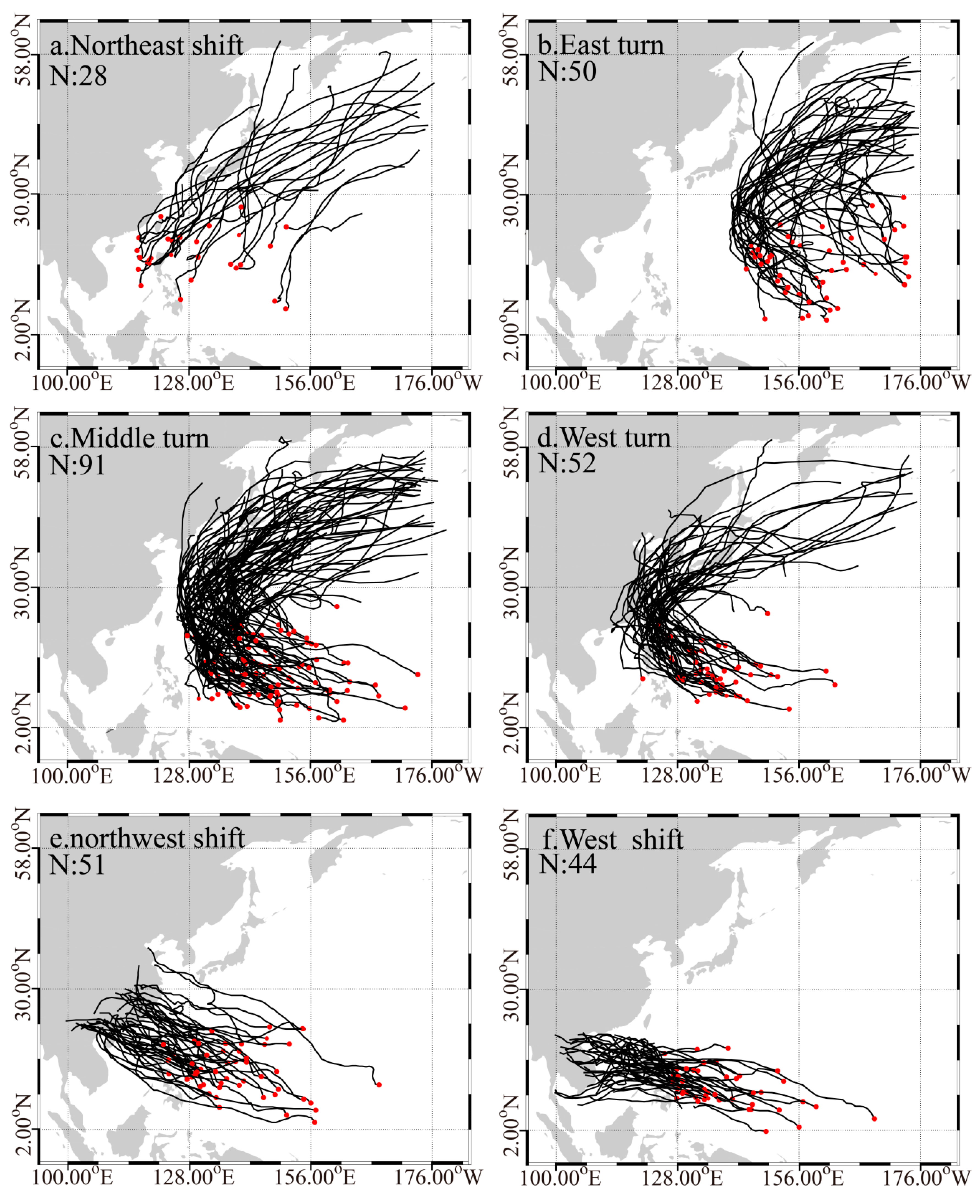
Figure 4.
The average result of SWH from the WW3 for each type of typhoon paths from 1998 to 2018, in which the black polylines represent the typical paths for each type of typhoon paths. (a) Northeast shift; (b) east turn; (c) middle turn; (d) west turn; (e) northwest shift; and (f) west shift.
Figure 4.
The average result of SWH from the WW3 for each type of typhoon paths from 1998 to 2018, in which the black polylines represent the typical paths for each type of typhoon paths. (a) Northeast shift; (b) east turn; (c) middle turn; (d) west turn; (e) northwest shift; and (f) west shift.
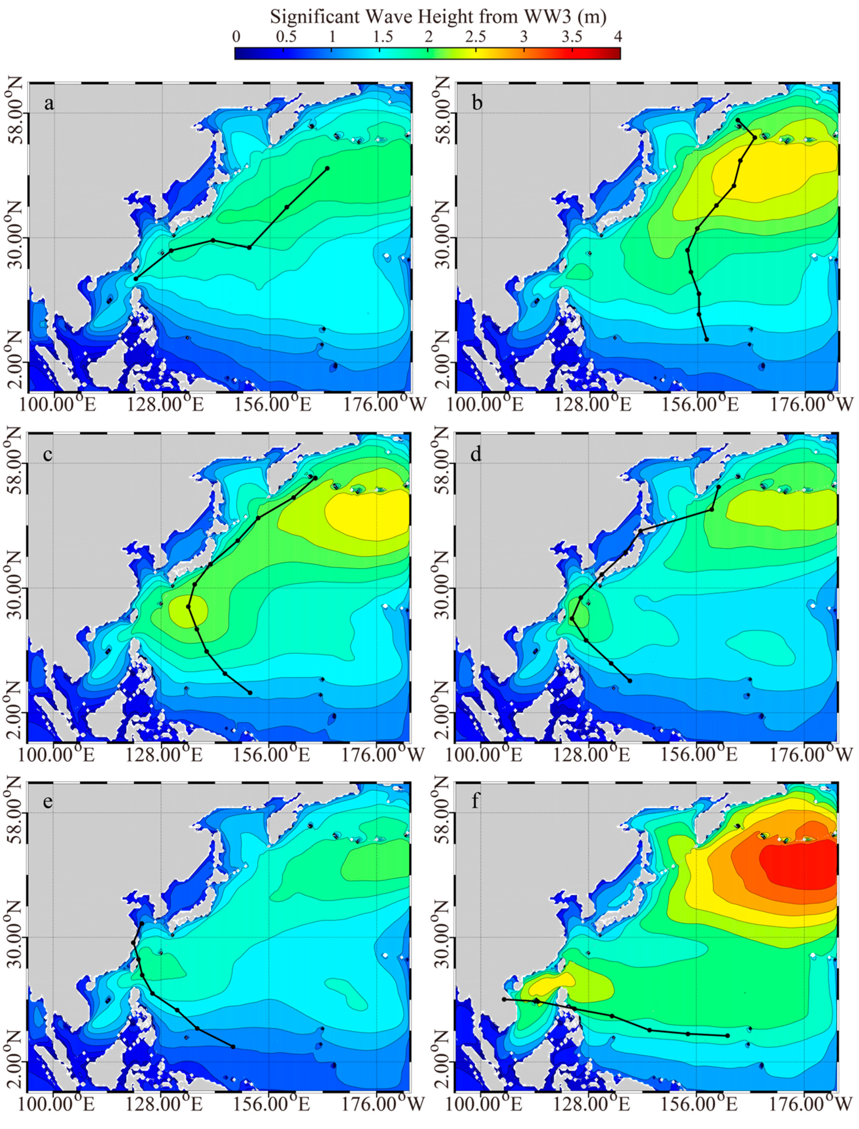
Figure 5.
The average result of mean wave period (MWP) from the WW3 for each type of typhoon paths from 1998 to 2018, in which the black polylines represent the typical paths for each type of typhoon paths. (a) Northeast shift; (b) east turn; (c) middle turn; (d) west turn; (e) northwest shift; and (f) west shift.

Figure 6.
The average result of MWL from the WW3 for each type of typhoon paths from 1998 to 2018, in which the black polylines represent the typical paths for each type of typhoon paths. (a) Northeast shift; (b) east turn; (c) middle turn; (d) west turn; (e) northwest shift; and (f) west shift.
Figure 6.
The average result of MWL from the WW3 for each type of typhoon paths from 1998 to 2018, in which the black polylines represent the typical paths for each type of typhoon paths. (a) Northeast shift; (b) east turn; (c) middle turn; (d) west turn; (e) northwest shift; and (f) west shift.

Figure 7.
The average result of wind-sea SWH from the WW3 for each type of typhoon paths from 1998 to 2018, in which the black polylines represent the typical paths for each type of typhoon paths. (a) Northeast shift; (b) east turn; (c) middle turn; (d) west turn; (e) northwest shift; and (f) west shift.

Figure 8.
The average result of swell SWH from the WW3 for each type of typhoon paths from 1998 to 2018, in which the black polylines represent the typical paths for each type of typhoon paths. (a) Northeast shift; (b) east turn; (c) middle turn; (d) west turn; (e) northwest shift; and (f) west shift.
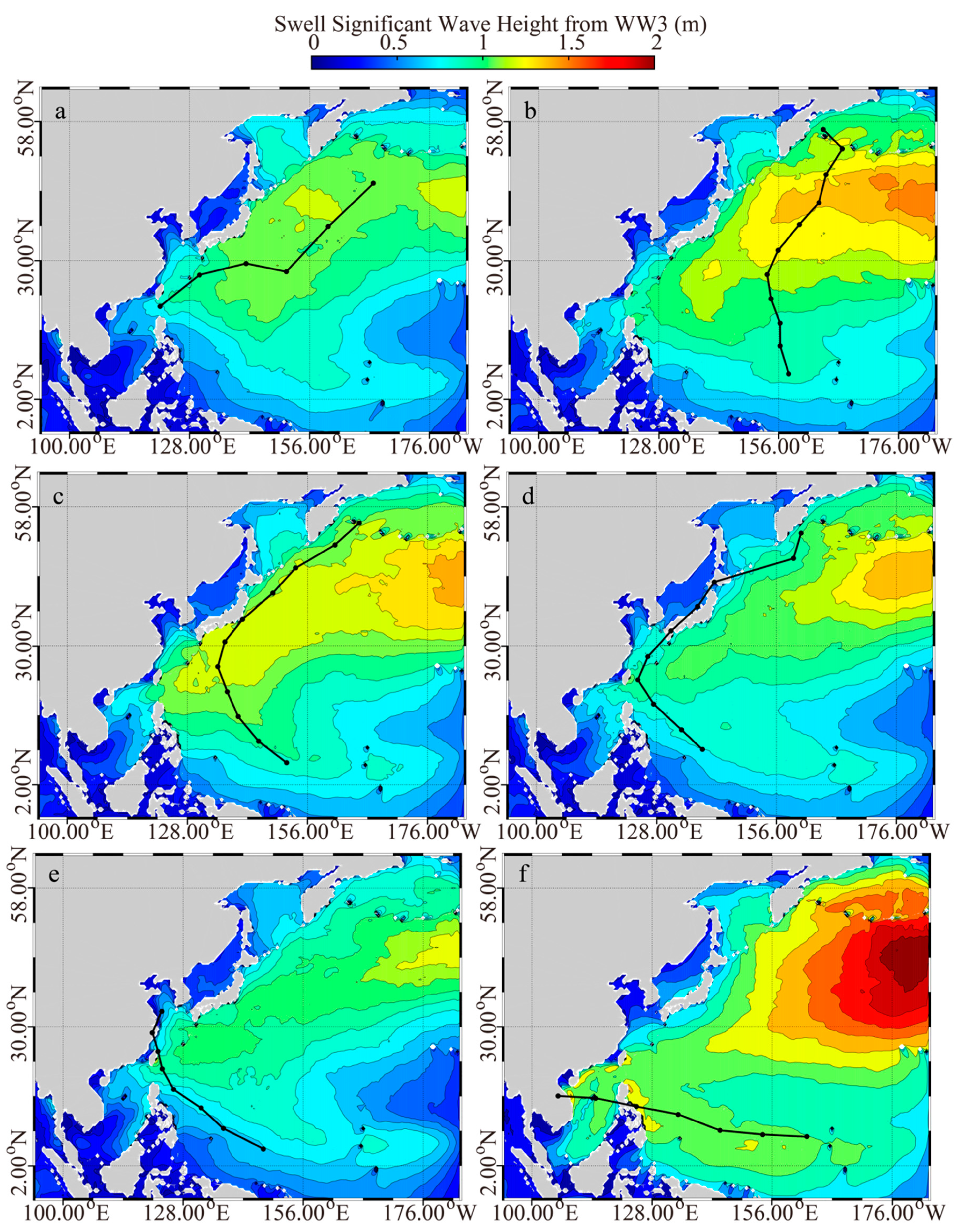
Figure 9.
Spatial distribution of the four dominant EOF modes for average SWH from 1998 to 2018. (a) The first mode; (b) the second mode; (c) the third mode; and (d) the forth mode.
Figure 9.
Spatial distribution of the four dominant EOF modes for average SWH from 1998 to 2018. (a) The first mode; (b) the second mode; (c) the third mode; and (d) the forth mode.
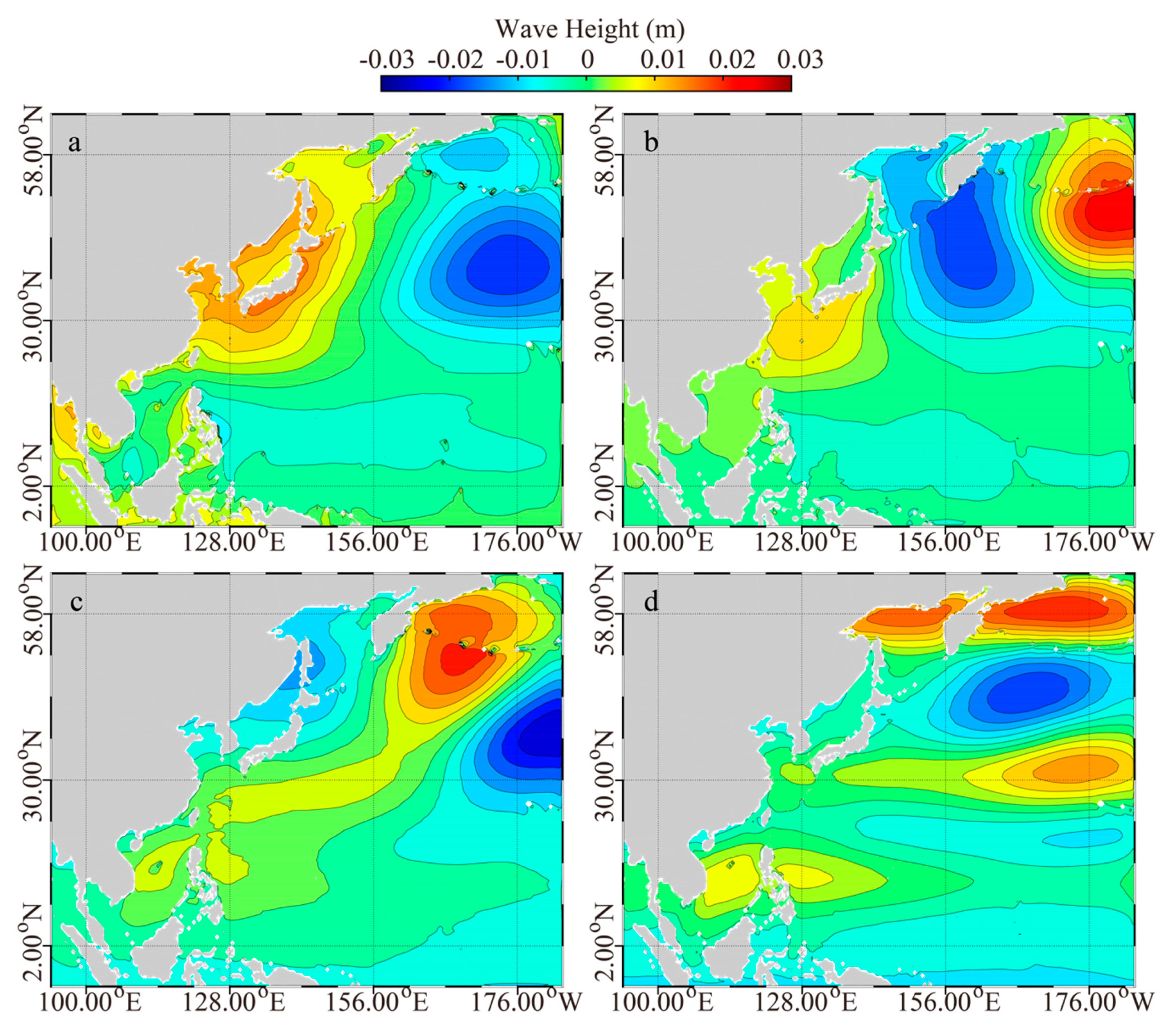
Figure 10.
Time series of the amplitudes of the four dominant EOF modes for average SWH from 1998 to 2018. (a) The first mode; (b) the second mode; (c) the third mode; and (d) the forth mode.
Figure 10.
Time series of the amplitudes of the four dominant EOF modes for average SWH from 1998 to 2018. (a) The first mode; (b) the second mode; (c) the third mode; and (d) the forth mode.
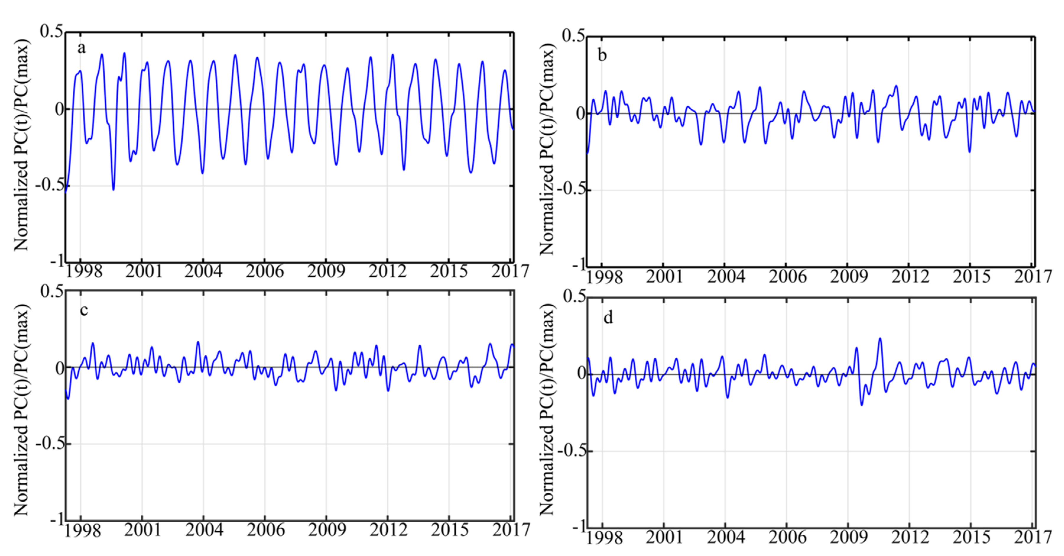
Figure 11.
The first mode principal components (PCs) part results in each path period. (a) Northeast shift; (b) east turn; (c) middle turn; (d) west turn; (e) northwest shift; and (f) west shift.
Figure 11.
The first mode principal components (PCs) part results in each path period. (a) Northeast shift; (b) east turn; (c) middle turn; (d) west turn; (e) northwest shift; and (f) west shift.

Table 1.
The information about the eigenvalue error method.
| Modes | ej | λj − λj + 1 | |
|---|---|---|---|
| 1 | 450.7115 | 7.4577 | 230.7340 |
| 2 | 219.9775 | 3.6398 | 36.5925 |
| 3 | 183.3850 | 3.0344 | 24.3827 |
| 4 | 159.0023 | 2.6309 | 26.6687 |
© 2020 by the authors. Licensee MDPI, Basel, Switzerland. This article is an open access article distributed under the terms and conditions of the Creative Commons Attribution (CC BY) license (http://creativecommons.org/licenses/by/4.0/).
Share and Cite
MDPI and ACS Style
Hu, Y.; Shao, W.; Wei, Y.; Zuo, J. Analysis of Typhoon-Induced Waves along Typhoon Tracks in the Western North Pacific Ocean, 1998–2017. J. Mar. Sci. Eng. 2020, 8, 521. https://doi.org/10.3390/jmse8070521
AMA Style
Hu Y, Shao W, Wei Y, Zuo J. Analysis of Typhoon-Induced Waves along Typhoon Tracks in the Western North Pacific Ocean, 1998–2017. Journal of Marine Science and Engineering. 2020; 8(7):521. https://doi.org/10.3390/jmse8070521
Chicago/Turabian StyleHu, Yuyi, Weizeng Shao, Yongliang Wei, and Juncheng Zuo. 2020. "Analysis of Typhoon-Induced Waves along Typhoon Tracks in the Western North Pacific Ocean, 1998–2017" Journal of Marine Science and Engineering 8, no. 7: 521. https://doi.org/10.3390/jmse8070521
Note that from the first issue of 2016, this journal uses article numbers instead of page numbers. See further details here.