Numerical Study on Wave Radiation by a Barge with Large Amplitudes and Frequencies


Research Center of Fluid Machinery Engineering and Technology, Jiangsu University, Zhenjiang 212013, China
*
Author to whom correspondence should be addressed.
J. Mar. Sci. Eng. 2020, 8(12), 1034; https://doi.org/10.3390/jmse8121034
Submission received: 16 November 2020
/
Revised: 14 December 2020
/
Accepted: 14 December 2020
/
Published: 19 December 2020
(This article belongs to the Section Ocean Engineering)
Abstract
:A two-dimensional boundary element method is used to study the hydrodynamics of a single barge with prescribed motions of large amplitudes and high frequencies. The wave radiation problem is solved in the time domain based on the fully nonlinear potential flow theory. For numerical simulations, special treatments like plunging wave cutting and remeshing approaches are presented in detail. The numerical schemes are verified through comparing with analytical results. Both the generated outgoing wave amplitudes and hydrodynamic coefficients can be calculated with sufficient accuracy. Then, we focus on large heave, sway and roll motions to investigate the nonlinear effects on hydrodynamic forces, respectively. In particular, the heave motion with two frequencies is also simulated to study the interactions between results at different frequencies. It is interesting to see the sum and difference frequency components and the envelopes in time histories as a result. For forces caused by forced sway or roll motions, there are only even-order harmonics for vertical forces and only odd-order harmonics for horizontal forces. Finally, a single body with combined sway, heave and roll motion is studied to examine the interactions between motion modes.
1. Introduction
The wave–body interaction problem has long been one of the focuses of hydrodynamics. The study starts from wave interactions with one single body. The understanding of the physical mechanism of hydrodynamic interaction of one body can shed light on the wave interactions with multiple bodies. The study on radiation problem can provide features of hydrodynamic properties of loads acting on the ocean structures and deformations of free surface profile.
The wave radiation problem is related to a rigid body in forced motions in otherwise calm water, which can generate outgoing waves. The oscillating fluid pressure resulting from the fluid motions and radiated waves is the source of hydrodynamic forces. The study of wave radiation problem dates at least back to Ursell [1]. He studied the harmonic heave motion of a horizontal circular cylinder in infinite water depth. The very long cylinder assumption made the problem to be reduced to two-dimensional (2D). Later, Kim [2] proposed a solution of the potential problem associated with the harmonic oscillation of an ellipse (2D) or ellipsoid (3D). Green’s function was introduced to represent the potential as the solution of an integral equation, which was obtained numerically. The hydrodynamic coefficients of all six motion modes were provided. Black et al. [3] calculated the radiation problem including heave, sway and roll of a rectangular section (2D) and a vertical circular cylinder (3D) by employing Schwinger’s variational formulation. An analytical solution to the heave radiation of a rectangular body was presented by Lee [4], who divided the whole fluid region into three sub-regions and solved the nonhomogeneous boundary value problem separately. Li et al. [5] considered the radiation problem of a circular cylinder submerged below an ice sheet with a crack. Deng et al. [6] analytically studied the variations of added masses and damping coefficients for surge, heave and pitch modes of a T-shaped breakwater. All the above-mentioned studies were based on the linearized water-wave theory. In order to consider nonlinear effects, second-order theory was developed. Typical works include: Lee [7] for semi-circular and U-shaped cylinders in heave motion and Papanikolaou and Nowacki [8] for arbitrary cylinders in heave, sway and roll motion. Isaacson and Ng [9] presented a 2D second-order solution in the time domain. The method was applicable to arbitrary body shapes under three motion modes. Wu [10] did a second-order study on a submerged horizontal circular cylinder undergoing heave, surge and circular motion.
With the demand for practical engineering applications and the rapid development of high- performance computers, fully nonlinear potential flow theory in the time domain dominates the study of radiation problem. Wu and Eatock Taylor [11] considered a 2D submerged circular cylinder subjected to forced periodic sway or heave motion. Domain decomposition technique was also used to satisfy the radiation condition on the truncated boundaries. Maiti and Sen [12] presented and discussed the heave radiation forces for both rectangular and triangular hull. A 3D vertical cylinder subjected to periodic oscillation in the open sea and in a channel were studied by Hu et al. [13] using the finite element method. Bai and Eatock Taylor [14] investigated truncated cylinder undergoing forced heave, surge and pitch with different amplitudes and frequencies. Wang et al. [15] considered a flared cylinder subjected to forced periodic sway or heave motions, with three different amplitudes, in an open sea. Zhou et al. [16] numerically investigated wave radiation by a vertical cylinder using a higher-order boundary element method. Zhou et al. [17] further carried out numerical experiments for a submerged sphere in heave motion and a truncated flared cylinder undergoing heave and pitch motions. Sun et al. [18] studied the prescribed rotation of a flap in calm water and with incoming waves, which was a common form in the wave energy sector. Li et al. [19] considered a floating barge undergoing forced sway motion and under incoming waves at the same time.
Previous studies have focused on wave radiation by a single body with different shapes, i.e., circular, triangular, rectangular, T-shaped and U-shaped cylinder, ellipse, ellipsoid, sphere and flared structures. The purpose of this study is to investigate the effect of radiation motion amplitude and frequency on the hydrodynamic performance of a rectangular barge. The remaining part of this paper is organized as follows. Section 2 gives the mathematical model and formulations of the radiation problem based on potential flow theory. Particularly, some special numerical treatments, i.e., plunging wave cutting and remeshing approaches are proposed in detail. Section 3 provides results and discussions for a barge of different amplitudes in heave, sway and roll motions to look at the nonlinear effects, respectively. A single body with combined sway, heave and roll motion is studied to examine the interactions between motion modes. Conclusions are given in Section 4, which highlights the main conclusions and contributions of the present study.
2. Mathematical Model and Its Numerical Implementation
The wave–body interaction problem is studied through velocity potential theory. This implies that the fluid is inviscid and the fluid motion is irrotational. In addition, the wave radiation problem is restricted to two dimensions. Assuming that the flow variation in the cross-sectional plane is much larger than that in the longitudinal direction, the three-dimensional problem can be simplified to a two-dimensional problem.
2.1. Governing Equations and Boundary Conditions
The physical problem of wave interactions with a single body is shown in Figure 1. The whole free surface is denoted as . The body of the rectangular shape has width and initial draught , which is measured from the still water level. The right-handed Cartesian co-ordinate system is employed with the -axis directing vertically upwards and the -axis lying in the still water surface from left to right. The origin is selected at the center line of the body. The water depth is denoted as . The center of gravity lies in the center line and is below the still water level. ‘Non-reflecting’ boundary conditions are applied on the truncated boundaries . The governing equation and the boundary conditions of the wave interaction problem are presented as below.
Since velocity potential exists, the mass continuity equation is reduced to the Laplace equation
On the free surface , expressed as , there exist both kinematic and dynamic conditions. Mathematically, in the Eulerian form, they can be expressed as
And in their Lagrangian form, they have
where is the material derivative following a given fluid particle.
On the wetted body surface , impermeable condition should be satisfied because no fluid particle can penetrate or leave the rigid body surface. It implies that the normal velocity of the fluid particle equals the normal component of the body surface velocity. Therefore, it yields
where represents the partial differentiation along the normal direction to the body surface, pointing out of the fluid domain. denotes the translational velocities of the body motion in the and direction, respectively. is the rotational velocity about the body’s rotational center, which is positive in the anticlockwise direction. is the position vector in the body-fixed system relative to the rotational center. The impermeable condition also applies to the sea bottom and the two truncated boundaries , which gives
For initial conditions, since the outgoing wave is excited by the body’s motion, the water is assumed to be undisturbed initially. Thus, the initial conditions on the free surface have the form
The above equations completely define the initial-boundary value problem (IBVP) for velocity potential . The whole flow field information including velocity and pressure field can be obtained after solving the IBVP.
To satisfy the radiation condition, an artificial damping zone is added to minimize the reflection of the truncated boundary . This is achieved by adding a damping term in Equation (3) artificially. So, they become
in which is the damping coefficient
The two parameters and are to control the damping strength and length, respectively. is the wavelength obtained from the dispersion relation, and is the oscillation frequency of the body motion. The performance of the damping zone depends on the combination of and . The criterion for appropriate and is to make sure that the radiated outgoing waves damp out gradually inside the damping zone and completely vanish at the truncated boundary. A detailed example of the selection of and for a single floating body is given by Tanizawa’s [20] study.
2.2. Hydrodynamic Forces and Moments
The hydrodynamic forces on the body can be obtained by direct integration of the pressure over the instantaneous wetted body surface . The pressure in the fluid can be determined through Bernoulli equation
The hydrodynamic forces and moments acting on the structures are then obtained through
In Equation (9), the time derivative of velocity potential, , is not explicitly given even when has been found. The auxiliary function approach [21,22] is adopted to circumvent the need for calculating so that the hydrodynamic forces can be obtained directly.
2.3. Numerical Procedures
The initial boundary value problem of velocity potential is solved by the boundary element method (BEM), which is derived based on Green’s second identity
where is the solid angle at point , stands for the closed boundary of the fluid domain (consisting of free surface, wetted body surface, truncated boundaries and sea bottom). Moreover, denotes the distance between two points and . Equation (11) is usually referred to as the boundary integral equation, which establishes a relationship between unknown at any point and the values of and on the boundary. For a 2D problem, the fluid boundary can be discretized into a number of straight line segments. Within each segment, formed by two neighboring nodes, introduce a natural coordinate along it, and postulate and as the linear interpolation of the values of the two nodes. Then, rewrite Equation (11) according to the newly discretized boundary, we could obtain
in which
denotes the total number of elements, and and are shape functions.
Finally, applying all the boundary conditions and moving all the unknown terms to the left-hand side and known terms to the right, we can get the matrix equation
The subscript denotes that the Neumann condition is applied on the corresponding boundaries and . Solving the equation above, the velocity potentials on and normal derivatives on the free surface at a given time can be obtained.
For numerical simulation in the time domain, the BEM should be used together with time stepping method. The BEM deals with the IBVP for velocity potential at a given time and the time stepping method updates the free surface position and the corresponding velocity potential to the next time. A second-order Runge–Kutta time integration is adopted to perform the updating. Let be expressed by a function (the actual form of the derivatives can be found in Equation (7)), then we have
where are known terms corresponding to time at the th step and are to be determined at time . is the time step. The fluid velocity on the free surface should be calculated as well after and are obtained in order to do the time integration. The calculation of fluid velocity is the same as in Li and Zhang [23]. Particular treatment is needed for intersection points, which belong to both free surface and wetted body surface. What is special here is that there are two different normal directions associated with the same point. Therefore, there are two normal derivatives at each intersection point. A common treatment is to split the normal derivative into two parts in accordance with the element which it belongs to [22]. When dealing with free surface nodes, only the part should be used. The velocity potential is continuous at any point. No special treatment is needed. The velocities at these intersection points are essential because they decide the accuracy of the wave run-up on the body and affect the evaluation of the hydrodynamic loads. Thus, the four-point Lagrangian interpolation, which gives higher accuracy, is used to calculate the velocities at intersection points instead of the linear interpolation. The velocities at the intersection points should be further refined according to the impermeable conditions since these nodes belong to the wetted body surface as well. This treatment not just ensures the higher order accuracy of the velocities, but also maintains smooth deformation of the free surface because the velocities at the intersection points are interpolated through that of the free surface nodes only.
2.4. Special Treatments
A thin jet can be formed along the body surface when the body is in large sway or roll motion. When it occurs, the free surface is very close to the body surface. This is likely to cause large numerical errors or even break down the simulation. A simple and common treatment is to cut the thin jet during simulation [24]. For long-time simulations, numerical error will be accumulated step after step. Saw-tooth instability may appear due to the nature of numerical method. To suppress this, the smoothing technique is used. In this paper, two schemes, the five-point-third-order smoothing algorithm [25] and energy smoothing scheme [26], are adopted for different initial meshes.
2.4.1. Plunging Wave Cutting
The plunging wave evolves with time and overturns until hitting the free surface underneath. It is slightly different form the plunging jet in Sun et al. [18] in terms of where the plunging happens. In their paper, the plunging jet occurs close to the body surface, while in this study the plunging wave appears relatively far from the body, usually beyond one wavelength. The simulation will break down once the plunging wave tip touches the free surface underneath. A simple treatment is to cut the plunging wave before it hits the main free surface. The judging condition should be the distance between the lowest point of the plunging wave (Point A in Figure 2 and the free surface underneath. When the distance ( is a factor to control the length of the jet to be kept, and is the reference element size on the free surface), part of the plunging wave should be cut. First, locate the turning point of the plunging wave (Point B in Figure 2) and then find Point C, which is the first node with value less than that of the turning Point . Connect points B and C as the new free surface. Obviously, new nodes need to be inserted between B and C.
2.4.2. Remeshing
After some periods of time, the nodes on the boundary may cluster or over stretch, which is a source of numerical inaccuracy and possible instability issue. To avoid over distorted elements, nodes on the boundary should be rearranged every several steps. Check the distance between two adjacent nodes. If they are too close, then delete one of the nodes. Otherwise, add nodes between the two existing nodes. Normally to is regarded as too large, and around is regarded as too small. is the original length of the element. The original nodes on the free surface follow the rule that fine and equal mesh is adopted in the close body region and the size increases gradually until the far-field. The remeshing aims to maintain this node distribution pattern. Considering an original node set on the free surface, the node set after remeshing is denoted as with known element size and the number of new nodes is unknown. The remeshing is performed in the following three steps. The first step is to calculate the whole arc length of the boundary to be re-discretized. Since we have known all the original nodes on the free surface and the length of each element , the total length of the first elements is calculated through
Accordingly, the whole length of the original node set is .
The second step is to determine the number of new nodes because the expected nodes’ distribution on the original curve is known. If we introduce another symbol to record the sum of the first elements of the remeshed curve, we have
And the total length of the remeshed node set is . Now, can be determined by the two inequalities
The final step is to distribute the new nodes on the free surface. The first and last nodes are unchanged during remeshing. So, we have
The following part demonstrates how to place nodes in between. There are three possibilities, as illustrated in Figure 3. The first one means that only one new node can be located on the original element . Thus, we have
then
The second possibility happens when the adjacent original nodes are too close, so no new node can be placed on the elements
then
is the number of original nodes to be skipped. The third possibility occurs when the adjacent nodes are too far away from each other, meaning that remeshing is not performed at every step. Let us say that new nodes can be placed on the element ( is an integer). That is
then
Special attention should be paid to the second to last node because the very last node is not calculated through the remeshing formula but remains the same as . Thus, the distance between these two nodes may not be desirable. To correct the possible issue of the distance, node is adjusted to the mid-point of and . That is
An advantage of this scheme is that it guarantees the quality of the mesh and is quite simple to implement in the programme since no additional equation needs to be solved. This, however, can only be used in 2D problems.
3. Numerical Results and Discussion
This section firstly provides the convergence study as validation tests. Then, we focus on large respective heave, sway and roll motions of a barge with different frequencies to look at the nonlinear effects due to the increase in amplitude of each degree of freedom. In particular, the heave motion with two frequencies is also simulated to study the interactions between results at different frequencies. In terms of the hydrodynamic loads, nonlinearity is manifested in the occurrence of the higher order harmonic forces. Finally, a single body with combined sway, heave and roll motion is studied to examine interactions between motions at three degrees of freedom. The hydrodynamic forces and moments of combined motion are compared with those of each single mode.
3.1. Convergence Study and Validation
The convergence study is done through the results of heave motion, in which the body is subjected to forced motion with displacement . The initial velocity of the body motion is not zero, which means an abrupt start and probably longer transient period. To allow for a gradual development of the flow field, the velocity is revised by multiplying a modification function [27]. In this paper, is adopted to ensure a steady state to be reached soon after the ramp time. is the modification time and is related to the period of the body motion . The displacement and acceleration of the body motion should be revised accordingly.
The vertical hydrodynamic force acting on the body can be obtained via Equation (10). The last term in the pressure represents the hydrostatic restoring pressure, which is excluded from the integration of vertical hydrodynamic force. To validate the numerical results, simulations are carried out under the same parameters as in Lee [4] and the results are compared with its linear analytical solutions. The case parameters in Lee [4] are and . The barge width . Since the analytical solutions are obtained through linear theory, the amplitude should be small to allow for the linearity assumption. equals in the following simulations. The frequencies of the body motion are set against , which is to compare the results in Lee [4] directly. is the wave number of the generated periodic wave and is linked with the frequency through the dispersion relation of finite water depth.
All simulations are carried out in a fluid domain with the body located at the center and with the truncated boundaries placed at , including the damping zone. The nodes are initially equally distributed on the wetted surface of the barge with element size . The free surface part near the body is discretized equally as well with . Away from the local zone on the free surface, the element size increases gradually until the far end. The biggest element on the free surface should not be larger than to ensure that there are at least 40 elements in each side of the damping zone. Larger elements of equal size are employed on the truncated boundaries and not changed during mesh convergence study, because they are far away from the barge. The nodes on the seabed right below the structure are placed equally with size and nodes on the rest of the seabed with size throughout all the simulations. During the simulation, the wetted body surface is remeshed every time step, keeping the segment size as . The whole free surface is remeshed and smoothed every 5 steps. The damping zone length is set as with damping strength for all the cases. The damping applied is quite effective. It minimizes the reflection and makes the radiated waves steady in time and periodic in time and space.
The convergence tests with reference to element size and time step are conducted based on the case when , because its frequency lies in the middle of the frequency range. The purpose of this test is to ensure accuracy and to provide reference parameters for the other simulations. The mesh size only refers to the element on the wetted body surface and the local region of the free surface. Three different meshes are tested with . The wave runup histories on the right side of the barge for the three meshes, which are given in Figure 4a, show that they are not sensitive to these element sizes. The hydrodynamic force on the barge, shown in Figure 4b, reveals that the coarser mesh causes a visible difference from the other two meshes. Considering the hydrodynamic forces, the mesh size is small enough to give convergent results and is chosen to test the temporal convergence. We then rerun the simulations with and and compare the corresponding wave runups and hydrodynamic forces on the barge in Figure 5. We can see that these curves are virtually coincident with each other, which means the larger time step is sufficient to guarantee the temporal convergence.
To ensure that the present numerical results are not only convergent but also reliable and accurate, they are compared with the linear analytical solutions presented in Lee [4]. Long-time simulation is conducted to guarantee the accuracy of the added mass and damping coefficients because they are calculated based on the periodic part of the hydrodynamic force history . Given that the hydrodynamic force history becomes periodic at , the dimensionless added mass coefficient and damping coefficient are determined through the following equation:
where is an integer. Free surface elevation is another feature to be considered in radiation problems. It is represented by the amplitude of generated outgoing waves. The generated wave amplitude is computed through the surface wave profile in zone , which excludes the local wave close to the body and waves in the damping zone. At each time instant, is determined as half of the vertical distance from the crest to trough. The comparison of dimensionless added mass, damping coefficients and generated wave amplitudes is made with analytical solutions and is given in Figure 6. The figure shows an excellent agreement, which indicates that the present numerical model and the code are quite capable of capturing the free surface elevation accurately. Generally speaking, the accuracy of the present numerical results is excellent since the variation tendency and values against for all the three physical variables and are very well captured compared with the analytical solutions.
3.2. Wave Radiation by a Single Motion Mode
The hydrodynamic properties of a floating barge depend on its body parameter and the motion mode. This section will investigate the nonlinear effects on the hydrodynamics against each motion mode, separately. The mesh used in the following simulations is the same as in the convergence study. The length variables are nondimensionalized by the barge width . Moreover, the water depth is assumed to be large compared to the generated wavelength and the body draught. The effect of water depth is ignored and should not be included in the results. The dimensionless parameter is therefore replaced by the body motion frequency . When analyzing the forces and moments, the contribution of static buoyancy is excluded.
3.2.1. Forced Heave Motion
The results will focus on the nonlinear effects on the hydrodynamic forces, due to the increase in the amplitude of the body motion. The nonlinearity can lead to the existence of higher harmonic force components. The superposition of these higher harmonic components makes the total force history irregular, as illustrated in Figure 7a, which is for and at different oscillation amplitudes. denotes the nondimensional frequency for a specific case in the following study. Figure 7b gives their corresponding Fast Fourier Transform (FFT) analysis and shows the amplitudes of the components. It is observed clearly from the figure that the higher harmonic force becomes more pronounced as the oscillation amplitude increases. The first harmonic force, however, still makes up a dominant proportion of the total force. In addition, the phase angle of the total force is not affected by the amplitude as observed in Figure 7a.
For heave motion with , the cases of amplitude are also simulated. Since the amplitude is very large compared to the draught, the bottom of the body will emerge from water occasionally during simulation if the frequency is also high. This will result in the breakdown of the calculation. Simulations show that the frequency should be lower than to keep the body bottom staying in the water. The comparison of vertical forces with different amplitudes when is shown in Figure 8a. It can be seen that the larger the amplitude, the bigger the force’s peak value. The analysis of their high harmonic components can be done through FFT and is presented in Figure 8b. The second and third harmonic forces grow as the amplitude increases. However, they are still very small compared to first harmonic force even if the amplitude is as large as three quarters of the draught.
The nonlinear features will be more complicated and interesting if the heave motion has multiple frequencies since there will be interactions between components at different frequencies. Let us consider the case with two frequencies. The displacement of the body is expressed as . The amplitudes at both frequencies are set as the same with and . The above calculations have shown that the amplitude of body motion cannot be large in order to keep the simulations running. One of the frequencies, denoted as , is set as . The second frequency is taken as 0.8, 1.05 and 1.2, respectively. The vertical force histories, given in Figure 9a, show clearly the envelope pattern. The period in the graph corresponds to the higher one of the two frequencies. The apparent difference lies in the period of the envelope . For and 1.2, is nearly the same because in both cases and depends on their difference. So, when is close to , the period of envelope becomes very long.
In order to obtain the frequency spectrum of the vertical forces, FFT is performed and given in Figure 9b. The primary frequency components are marked in the figure. As we can see, there exist both sum and difference frequencies in addition to the two excitation frequencies and . Due to the existence of difference frequency , the envelope of vertical force shows a period longer than that of heave motion. These sum and difference frequencies reflect the nonlinear interaction between motions. The spectral analysis of wave runups on the body is also given in Figure 10. The same feature as vertical forces is shown.
3.2.2. Forced Sway Motion
The displacement is prescribed as During simulations, water spray will occur on the free surface when the amplitude of sway motion is large or the frequency of motion is high. Thus, spray cutting is needed, which is done through the method detailed in Section 2. The simulations are conducted with and , which corresponds to relatively slow motion because of the low frequency. The horizontal and vertical force histories at different draughts are given in Figure 11a,c, respectively. Any differences in these cases are due to the body draughts. It can be seen that the horizontal forces are significantly affected by the draughts. This is because horizontal forces are mainly attributed to the pressure on the side walls, whose magnitudes are directly related to the body draughts. However, the vertical forces are due to the hydrodynamic pressure on the bottom. The FFT analysis of these horizontal and vertical forces is provided in Figure 11b,d, respectively. It is interesting to notice that the leading component of vertical force is the second harmonic force and there are no even order components of horizontal forces. Furthermore, there are large negative mean vertical forces caused by sway motion at this low frequency.
We then consider the cases when the body oscillates very fast horizontally with large frequency and . Their horizontal and vertical force histories are illustrated in Figure 12a,c, respectively. Clear differences can be seen on the peaks and troughs of horizontal forces for different draughts because of the increase in frequency when comparing Figure 11a with Figure 12a. Double peaks appear for deep draught with high frequency. In terms of vertical forces, the high frequency makes them of shallower draught considerably larger than that of deeper draught, while the low frequency allows the draught to have little effect on them. This may be because the hydrodynamic pressure on the bottom is larger closer to the free surface and the high frequency magnifies this difference greatly. The FFT analysis of these forces, which is provided in Figure 12b, gives the frequency components of them. In particular, it is observed in the four spectral graphs, including the above two graphs for , that there are only even-order harmonic forces for vertical forces and only odd-order harmonic forces for horizontal forces. In fact, this phenomenon is discovered and shown mathematically by Wu [28].
Finally, we will examine the effect of sway motion amplitude with and . The FFT analysis of their horizontal and vertical forces is given in Figure 13a,b, respectively. The amplitude of each order of harmonic force of both horizontal and vertical forces grows with the increase in amplitude as expected. In particular, the fifth harmonic horizontal force and sixth harmonic vertical force become noticeable when the amplitude equals three quarters of the body breadth.
3.2.3. Forced Roll Motion
The roll motion is about the body’s longitudinal -axis and through the gravitational center, which is located at half of the draught below the still water. This means . The draught of the body is . The angular displacement of the body can be expressed as is the amplitude of roll motion. Three amplitudes , and are considered. For a practical ship, a rolling angle of is regarded as very large. However, such a scenario still needs to be considered as it poses great danger to ship safety.
During the simulations, a thin jet can be formed along the body surface because of the impact on the free surface. It is cut in this study. The time histories of horizontal and vertical forces and moments are plotted in Figure 14a,c and e for , respectively. The forces and moments are already normalized by . Therefore, any differences in these cases are due to nonlinear effects, which affect vertical forces the greatest. Additionally, the increase in amplitude will not cause phase shifts of forces. The FFT analysis of forces and moments is provided in Figure 14b,d,f, respectively. According to the conclusions made in Wu [28], there should be only odd-order harmonic components existing in horizontal forces and moments, while only even order-harmonic components should be occurring in vertical forces as observed in sway motion cases. The spectral analysis of these forces shows that the present numerical results are consistent with the above statement, especially the horizontal forces. The same observation is made when the frequency is as high as . Their frequency components are analyzed and shown in Figure 15. One may notice that there are even-order harmonic moments and a small first-order harmonic vertical force when the amplitude of the roll motion is large. This may be because the jet cutting treatment performed damages the mirror images formed about the wetted body surface to some extent.
3.3. Wave Radiation by Combined Motion
We have investigated each degree of freedom. The combined motion is now considered. The draught of the body is . The displacement of each degree of freedom is specified as before and with the same frequency and no phase difference. The relative phase differences among motion modes are not considered in the present study. The amplitude of both heave and sway motion is . The amplitude angle of roll motion is , or 11.46°. The purpose of this study is to examine the interactions between motion modes. The hydrodynamic forces and moments are compared with that of each single mode.
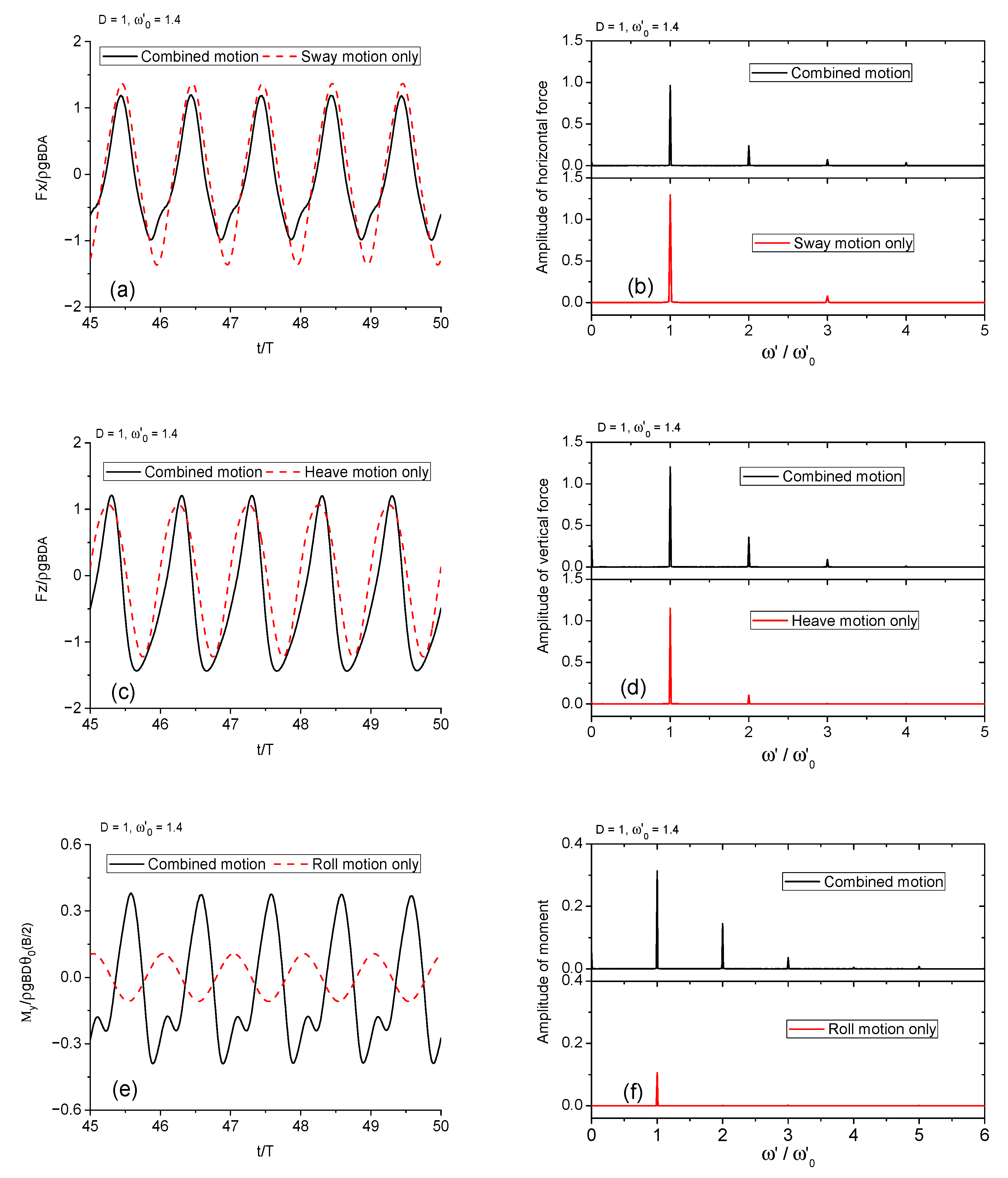
The frequency of is first simulated. The comparisons of forces and moments are provided in Figure 16. The horizontal force of combined motion is actually a little smaller than that of sway motion only. However, a small second harmonic component appears in the combined motion. As for the vertical force, its mean value and the second harmonic force is excited to a large extent compared to the vertical force in pure heave, while the first harmonic force is unaffected. This can be explained by the conclusions in the previous subsection. Specifically, the sway and roll motion can only trigger the frequency components at of vertical force. The multiple mode interactions affect the moment the greatest, as shown in Figure 16e,f. This is because the moment is dependent on both horizontal and vertical forces. The second case is when the frequency of combined motion is set as high as . The motion of the free surface within one period is illustrated in Figure 17. Sprays of the free surface can be seen on both sides of the body. They develop with time and travel in the space. They are cut before touching the main fluid underneath. The hydrodynamic forces and moments are then compared with single mode results in Figure 18. The horizontal force is still smaller in magnitude compared to sway motion force. It, however, consists of more high-frequency components. In comparison, the vertical force and moment are both larger than those of the single mode and contain more high-frequency components, especially the moment. These conclusions are the same as the previous low frequency case.
4. Concluding Remarks
This paper mainly studies the wave radiation by a single body with large amplitudes and high frequencies through numerical simulations based on the fully nonlinear potential flow theory in the time domain. The associated initial boundary value problem is established in both the Eulerian and Lagrangian frameworks, which is solved by the boundary element method combined with the time stepping scheme. During simulations, some special numerical treatments are also applied to the free surface, such as remeshing, smoothing, thin jet and plunging wave cutting. In particular, new approaches for plunging wave cutting and remeshing are proposed in detail. They have advantages for dealing with meshes in two-dimensional problems. The numerical schemes are verified through comparing with analytical results. Cases of wave radiation by a single barge of different motion amplitudes and frequencies are considered. The findings below are all based on the results obtained from potential flow theory without considering the viscous effect.
For wave radiation by a single motion mode, we focus on heave, sway and roll motions to look at the higher order harmonics due to the increase in the body oscillation amplitude, respectively. The increase in the body motion amplitude can enhance the nonlinear effects of the radiation problem. For heave motion with two frequencies, it is interesting to see the sum and difference frequency components and the envelopes in time histories as a result. For forces caused by forced sway or roll motions, there are only even-order harmonics for vertical forces and only odd-order harmonics for horizontal forces. Additionally, the moment due to roll motion has only odd-order harmonics. For a single body with combined sway, heave and roll motions, the hydrodynamic forces and moments are compared with those of each single mode. The horizontal force of combined motion is actually a little smaller than that of sway motion only. However, a small second harmonic component appears in the combined motion. As for the vertical force, its mean value and the second harmonic force is excited to a large extent compared to the vertical force in pure heave, while the first harmonic force is unaffected.
Author Contributions
Y.L. (Yajie Li) developed models, analyzed results and wrote the manuscript; Y.L. (Yun Long) reviewed the results, edited the manuscript and acquired funding. All authors have read and agreed to the published version of the manuscript.
Funding
This research was funded by Senior Talent Foundation of Jiangsu University (Grant No. 18JDG036), the China Postdoctoral Science Foundation Funded Project (Grant No. 2019M651734), National Youth Natural Science Foundation of China (Grant No. 51906085), and Jiangsu Province Innovation and Entrepreneurship Doctor Project (2019).
Acknowledgments
The authors appreciate Jiangsu University for its funding and support. Special thanks go to G. X. Wu from University College London for his helpful discussions on this work.
Conflicts of Interest
The authors declare no conflict of interest.
References
- Ursell, F. On the heaving motion of a circular cylinder on the surface of a fluid. Q. J. Mech. Appl. Math. 1949, 2, 218–231. [Google Scholar] [CrossRef] [Green Version]
- Kim, W.D. On the harmonic oscillations of a rigid body on a free surface. J. Fluid Mech. 1965, 21, 427–451. [Google Scholar] [CrossRef]
- Black, J.L.; Mei, C.C.; Bray, M.C.G. Radiation and scattering of water waves by rigid bodies. J. Fluid Mech. 1971, 46, 151–164. [Google Scholar] [CrossRef]
- Lee, J.F. On the heave radiation of a rectangular structure. Ocean Eng. 1995, 22, 19–34. [Google Scholar] [CrossRef]
- Li, Z.F.; Wu, G.X.; Ji, C.Y. Wave radiation and diffraction by a circular cylinder submerged below an ice sheet with a crack. J. Fluid Mech. 2018, 845, 682–712. [Google Scholar] [CrossRef]
- Deng, Z.; Wang, L.; Zhao, X.; Huang, Z. Hydrodynamic performance of a T-shaped floating breakwater. Appl. Ocean Res. 2019, 82, 325–336. [Google Scholar] [CrossRef]
- Lee, C.M. The second-order theory of heaving cylinders in a free surface. J. Ship Res. 1968, 12, 313–327. [Google Scholar]
- Papanikolaou, A.; Nowacki, H. Second-Order Theory of Oscillating Cylinders in a Regular Steep Wave. In Proceedings of the 13th Symposium on Naval Hydrodynamics, Tokyo, Japan, 6–10 October 1980. [Google Scholar]
- Isaacson, M.; Ng, J.Y.T. Time-Domain Second-Order Wave Radiation in Two Dimensions. J. Ship Res. 1993, 37, 25–33. [Google Scholar]
- Wu, G.X. Second-order wave radiation by a submerged horizontal circular cylinder. Appl. Ocean Res. 1993, 15, 293–303. [Google Scholar] [CrossRef]
- Wu, G.X.; Eatock Taylor, R. Time stepping solutions of the two-dimensional nonlinear wave radiation problem. Ocean Eng. 1995, 22, 785–798. [Google Scholar] [CrossRef]
- Maiti, S.; Sen, D. Nonlinear heave radiation forces on two-dimensional single and twin hulls. Ocean Eng. 2001, 28, 1031–1052. [Google Scholar] [CrossRef]
- Hu, P.; Wu, G.X.; Ma, Q.W. Numerical simulation of nonlinear wave radiation by a moving vertical cylinder. Ocean Eng. 2002, 29, 1733–1750. [Google Scholar] [CrossRef]
- Bai, W.; Eatock Taylor, R. Higher-order boundary element simulation of fully nonlinear wave radiation by oscillating vertical cylinders. Appl. Ocean Res. 2006, 28, 247–265. [Google Scholar] [CrossRef]
- Wang, C.Z.; Wu, G.X.; Drake, K.R. Interactions between nonlinear water waves and non-wall-sided 3D structures. Ocean Eng. 2007, 34, 1182–1196. [Google Scholar] [CrossRef]
- Zhou, B.Z.; Ning, D.; Teng, B.; Bai, W. Numerical investigation of wave radiation by a vertical cylinder using a fully nonlinear HOBEM. Ocean Eng. 2013, 70, 1–13. [Google Scholar] [CrossRef]
- Zhou, B.Z.; Ning, D.; Teng, B.; Zhao, M. Fully nonlinear modeling of radiated waves generated by floating flared structures. Acta Mech. Sin. 2014, 30, 667–680. [Google Scholar] [CrossRef]
- Sun, S.Y.; Sun, S.L.; Ren, H.L.; Wu, G.X. Splash jet and slamming generated by a rotating flap. Phys. Fluids 2015, 27, 092107. [Google Scholar] [CrossRef]
- Li, Y.; Xu, B.; Zhang, D.; Shen, X.; Zhang, W. Numerical analysis of combined wave radiation and diffraction on a floating barge. Water 2020, 12, 205. [Google Scholar] [CrossRef] [Green Version]
- Tanizawa, K. Long time fully nonlinear simulation of floating body motions with artificial damping zone. J. Soc. Nav. Arch. Jpn. 1996, 180, 311–319. [Google Scholar] [CrossRef] [Green Version]
- Wu, G.X.; Eatock Taylor, R. The coupled finite element and boundary element analysis of nonlinear interactions between waves and bodies. Ocean Eng. 2003, 30, 387–400. [Google Scholar] [CrossRef] [Green Version]
- Xu, G.D.; Duan, W.Y.; Wu, G.X. Numerical simulation of water entry of a cone in free-fall motion. Q. J. Mech. Appl. Math. 2011, 64, 265–285. [Google Scholar] [CrossRef] [Green Version]
- Li, Y.; Zhang, C. Analysis of wave resonance in gap between two heaving barges. Ocean Eng. 2016, 117, 210–220. [Google Scholar] [CrossRef]
- Sun, H.; Faltinsen, O.M. The influence of gravity on the performance of planing vessels in calm water. J. Eng. Math. 2007, 58, 91–107. [Google Scholar] [CrossRef]
- Xu, G.D.; Duan, W.Y.; Wu, G.X. Simulation of water entry of a wedge through free fall in three degrees of freedom. Proc. R. Soc. Lond. 2010, 466, 2219–2239. [Google Scholar] [CrossRef]
- Wang, C.Z.; Wu, G.X. An unstructured-mesh-based finite element simulation of wave interactions with non-wall-sided bodies. J. Fluids Struct. 2006, 22, 441–461. [Google Scholar] [CrossRef]
- Isaacson, M.; Cheung, K.-F. Second order wave diffraction around two-dimensional bodies by time-domain method. Appl. Ocean Res. 1991, 13, 175–186. [Google Scholar] [CrossRef]
- Wu, G.X. A note on non-linear hydrodynamic force on a floating body. Appl. Ocean Res. 2000, 22, 315–316. [Google Scholar] [CrossRef]
Figure 1.
Sketch of the problem.
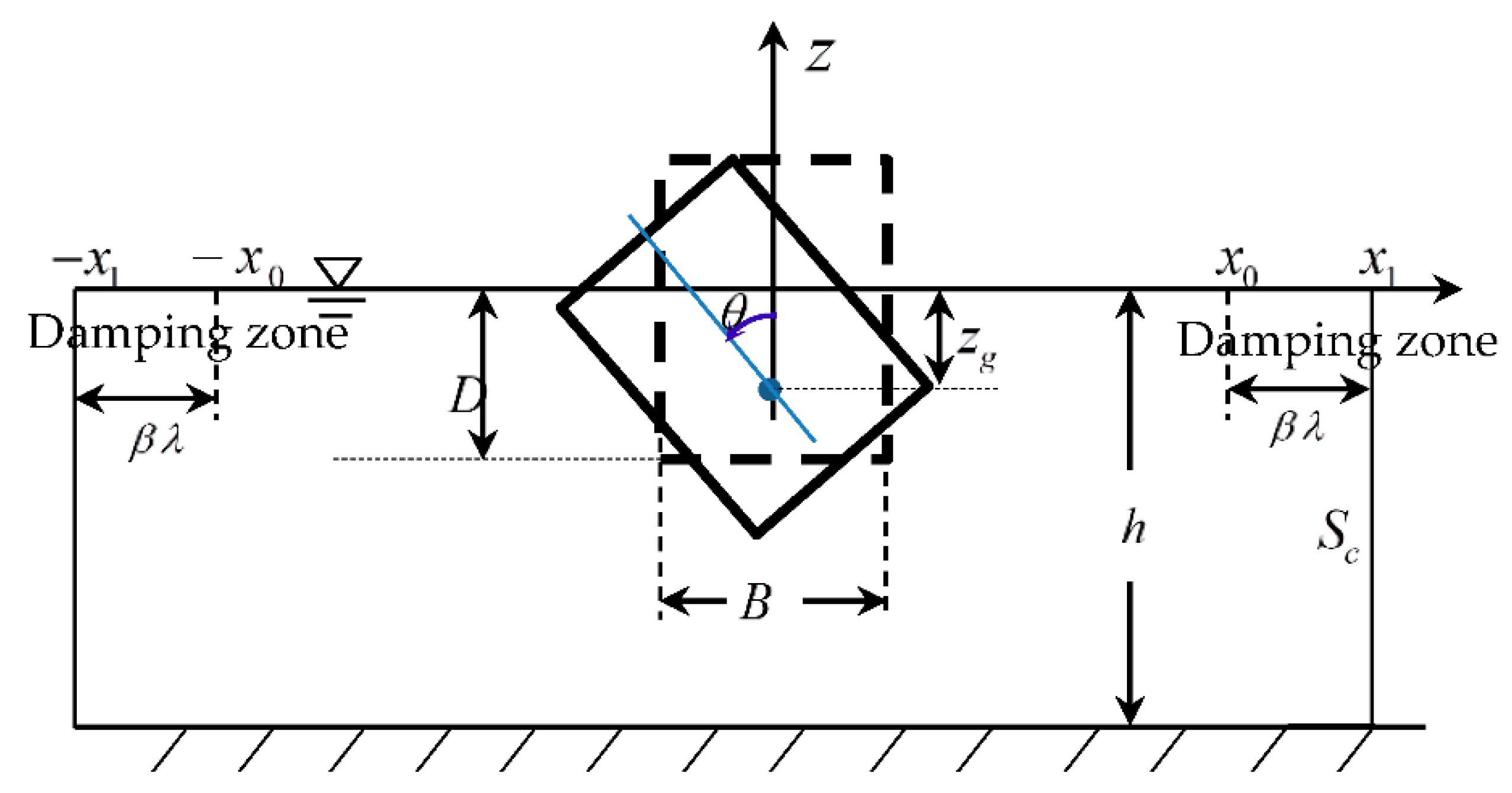
Figure 2.
Scheme of the plunging wave cut treatment.

Figure 3.
Schematic sketch of the three possibilities.
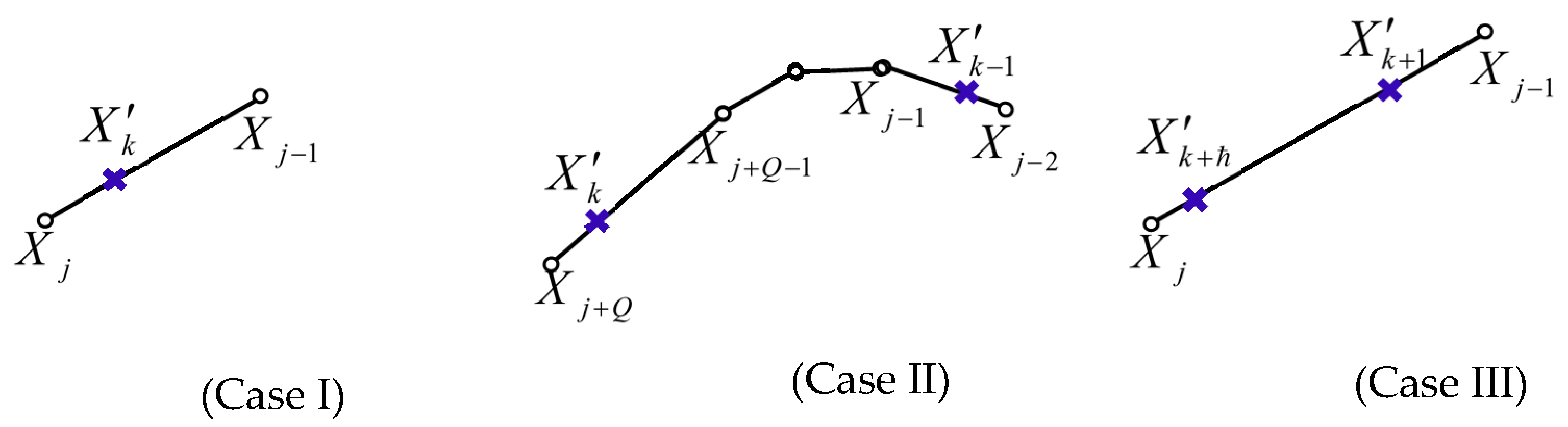
Figure 4.
Convergence study with element size.: (a) wave runup on the right side of the body; (b) vertical force on the body.
Figure 4.
Convergence study with element size.: (a) wave runup on the right side of the body; (b) vertical force on the body.
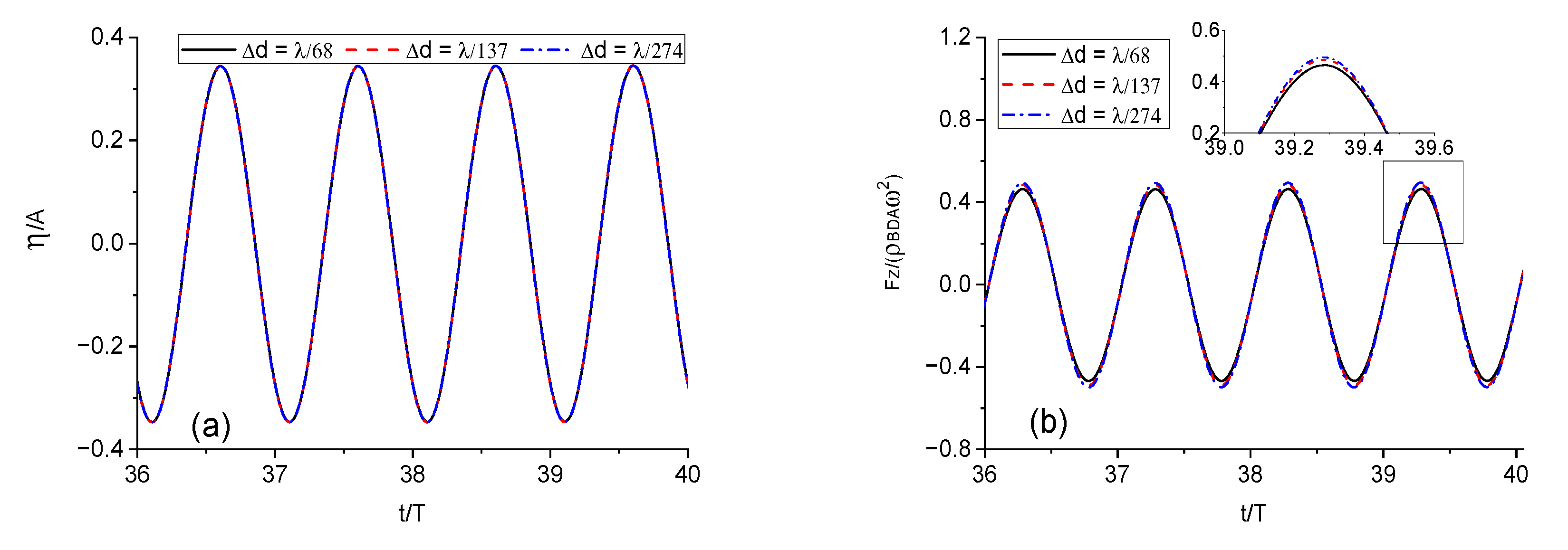
Figure 5.
Convergence study with time step: (a) wave runup on the right side of the body; (b) vertical force on the body.
Figure 5.
Convergence study with time step: (a) wave runup on the right side of the body; (b) vertical force on the body.
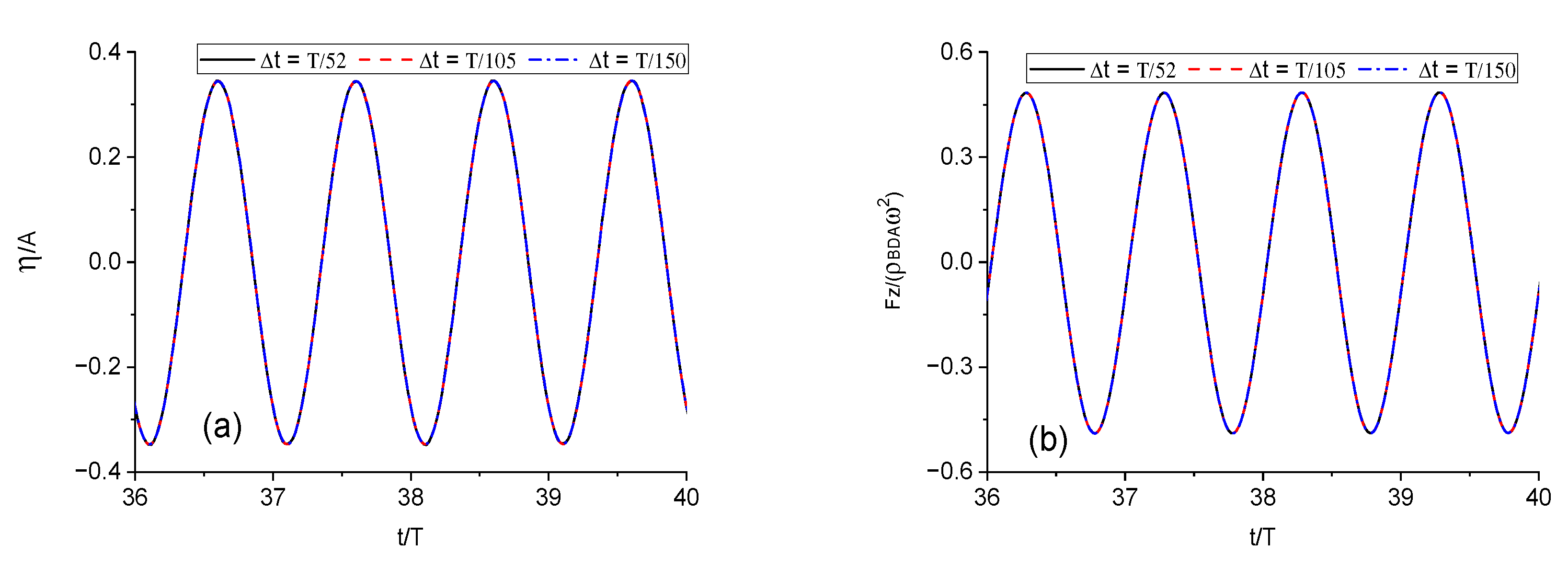
Figure 6.
Comparison of dimensionless added mass, damping coefficients and wave amplitude with analytical solution in Lee [4].
Figure 6.
Comparison of dimensionless added mass, damping coefficients and wave amplitude with analytical solution in Lee [4].
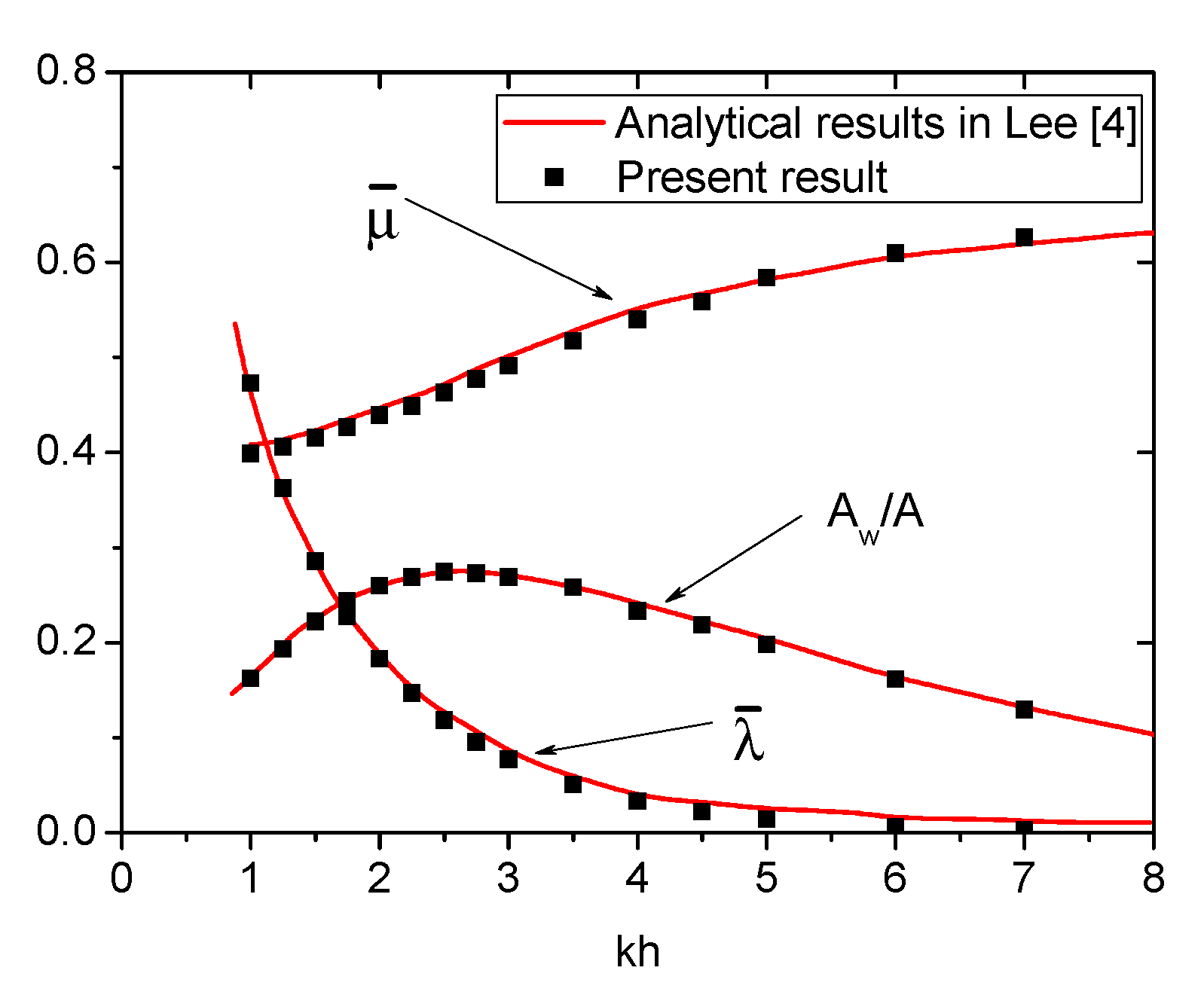
Figure 7.
Hydrodynamic force histories and their corresponding amplitude spectral analyses of , : (a) vertical force histories; (b) Fast Fourier Transform (FFT) analysis of the vertical forces.
Figure 7.
Hydrodynamic force histories and their corresponding amplitude spectral analyses of , : (a) vertical force histories; (b) Fast Fourier Transform (FFT) analysis of the vertical forces.
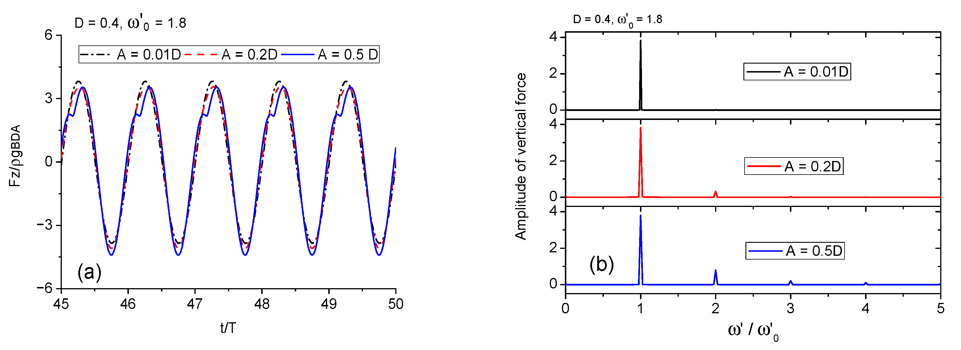
Figure 8.
Vertical force histories of different motion amplitudes and their corresponding spectral analyses when : (a) vertical force histories; (b) FFT analysis of these vertical forces.
Figure 8.
Vertical force histories of different motion amplitudes and their corresponding spectral analyses when : (a) vertical force histories; (b) FFT analysis of these vertical forces.
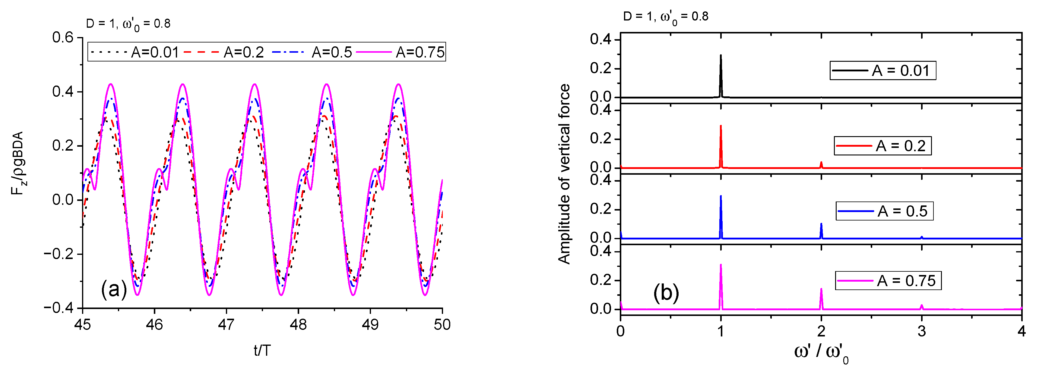
Figure 9.
Vertical force histories and their amplitude spectral analysis of heave motion with two frequencies: (a) vertical force histories; (b) FFT analysis of the vertical forces.
Figure 9.
Vertical force histories and their amplitude spectral analysis of heave motion with two frequencies: (a) vertical force histories; (b) FFT analysis of the vertical forces.
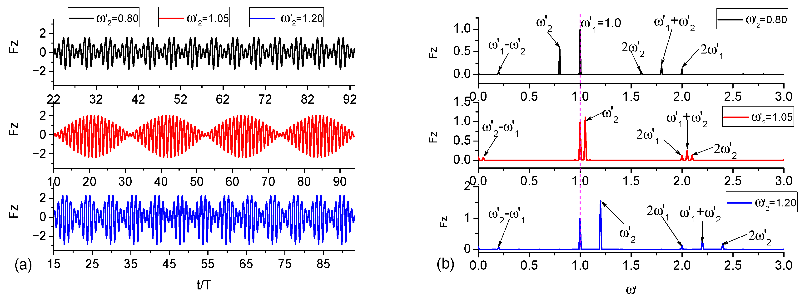
Figure 10.
Amplitude spectral analysis of wave runups of heave motion with two frequencies.
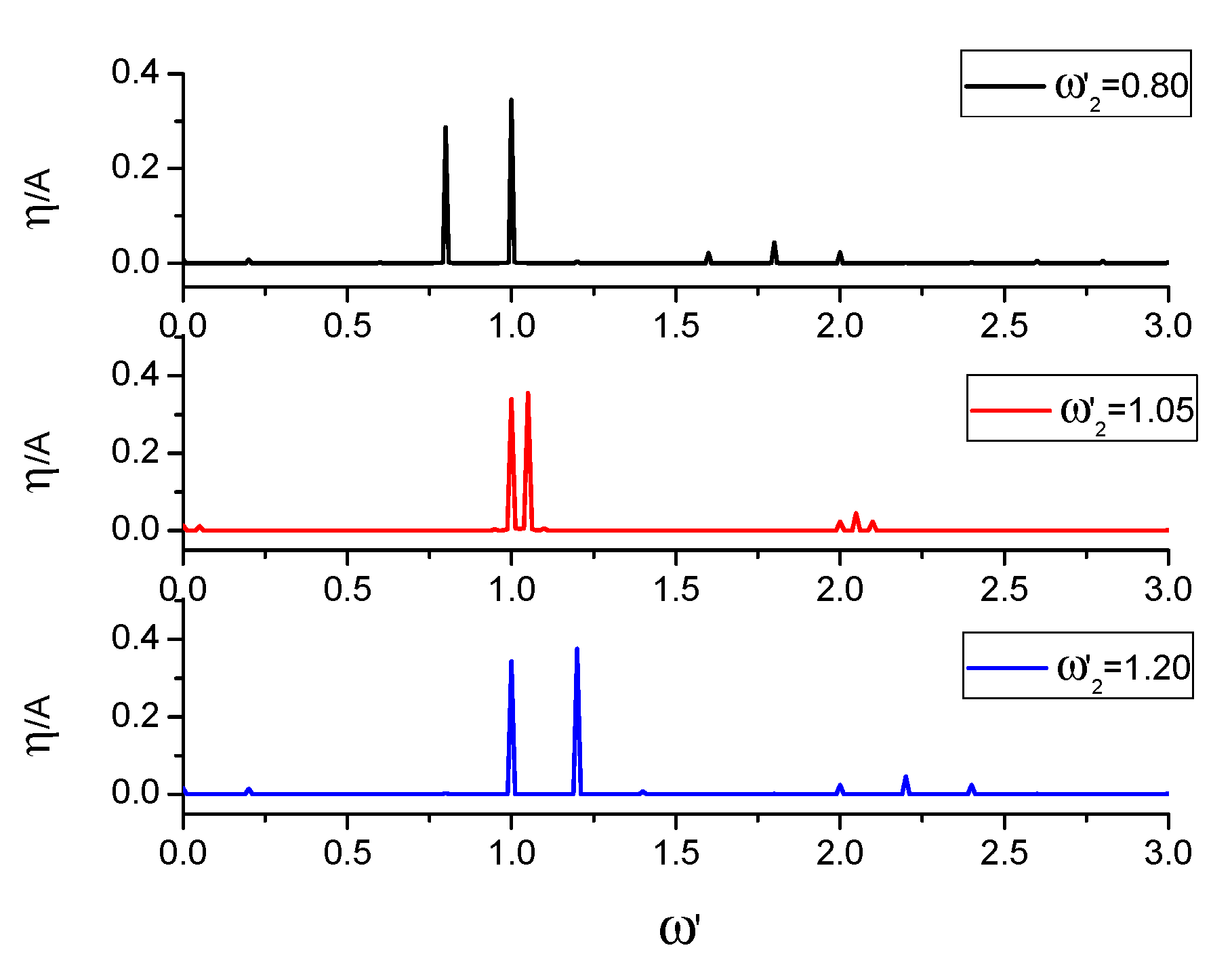
Figure 11.
Normalized force histories of different draughts and their FFT analysis when , : (a) horizontal force histories; (b) FFT analysis of horizontal forces; (c) vertical force histories; (d) FFT analysis of vertical forces.
Figure 11.
Normalized force histories of different draughts and their FFT analysis when , : (a) horizontal force histories; (b) FFT analysis of horizontal forces; (c) vertical force histories; (d) FFT analysis of vertical forces.
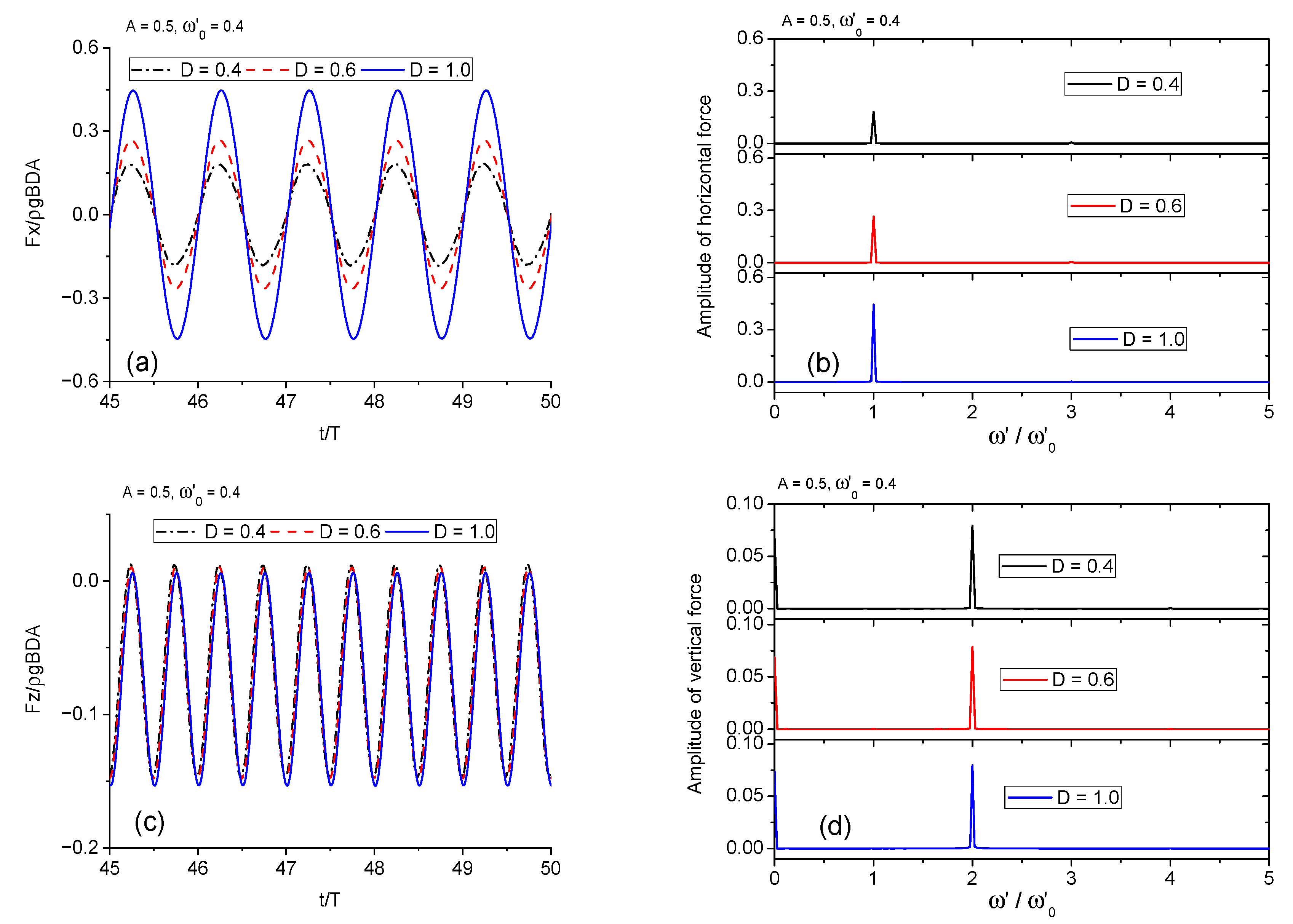
Figure 12.
Normalized force histories of different draughts and their FFT analysis when , : (a) horizontal force histories; (b) FFT analysis of horizontal forces; (c) vertical force histories; (d) FFT analysis of vertical forces.
Figure 12.
Normalized force histories of different draughts and their FFT analysis when , : (a) horizontal force histories; (b) FFT analysis of horizontal forces; (c) vertical force histories; (d) FFT analysis of vertical forces.

Figure 13.
FFT analysis of normalized forces of different amplitudes when , : (a) FFT analysis of horizontal forces; (b) FFT analysis of vertical forces.
Figure 13.
FFT analysis of normalized forces of different amplitudes when , : (a) FFT analysis of horizontal forces; (b) FFT analysis of vertical forces.
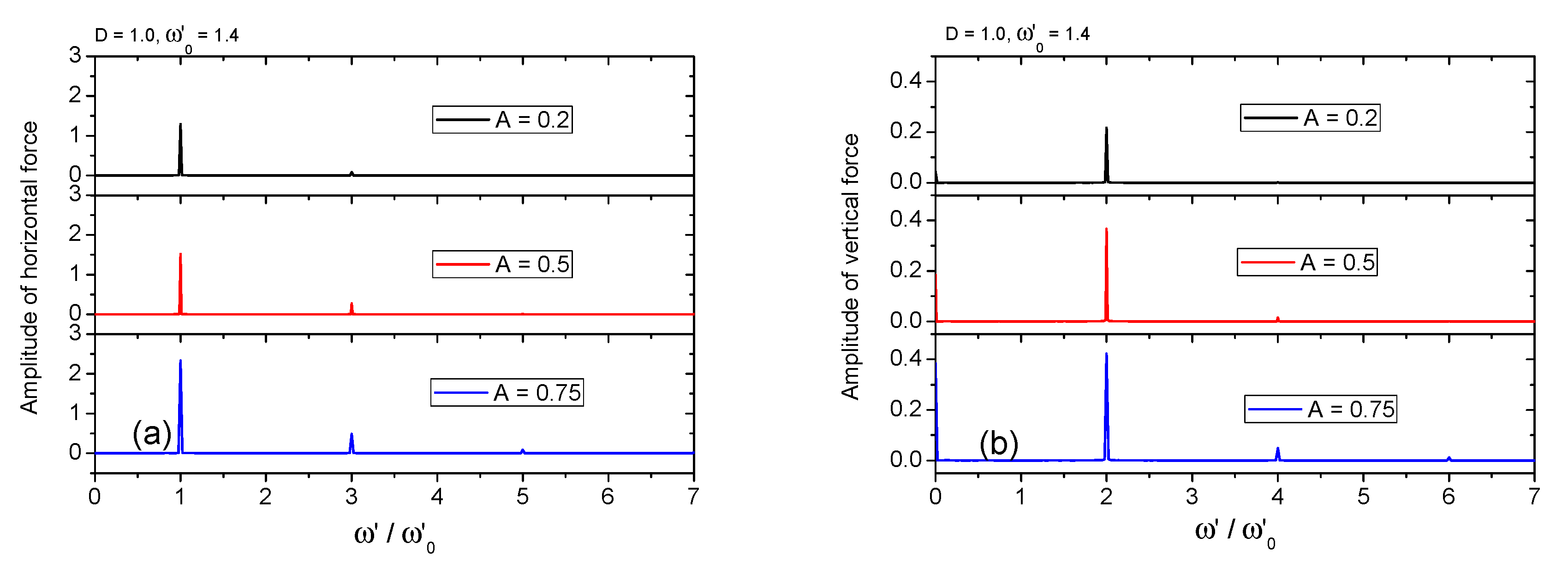
Figure 14.
Normalized forces and moments histories of different amplitudes and their FFT analysis when , : (a) horizontal force histories; (b) FFT analysis of horizontal forces; (c) vertical force histories; (d) FFT analysis of vertical forces; (e) moment histories; (f) FFT analysis of moment.
Figure 14.
Normalized forces and moments histories of different amplitudes and their FFT analysis when , : (a) horizontal force histories; (b) FFT analysis of horizontal forces; (c) vertical force histories; (d) FFT analysis of vertical forces; (e) moment histories; (f) FFT analysis of moment.
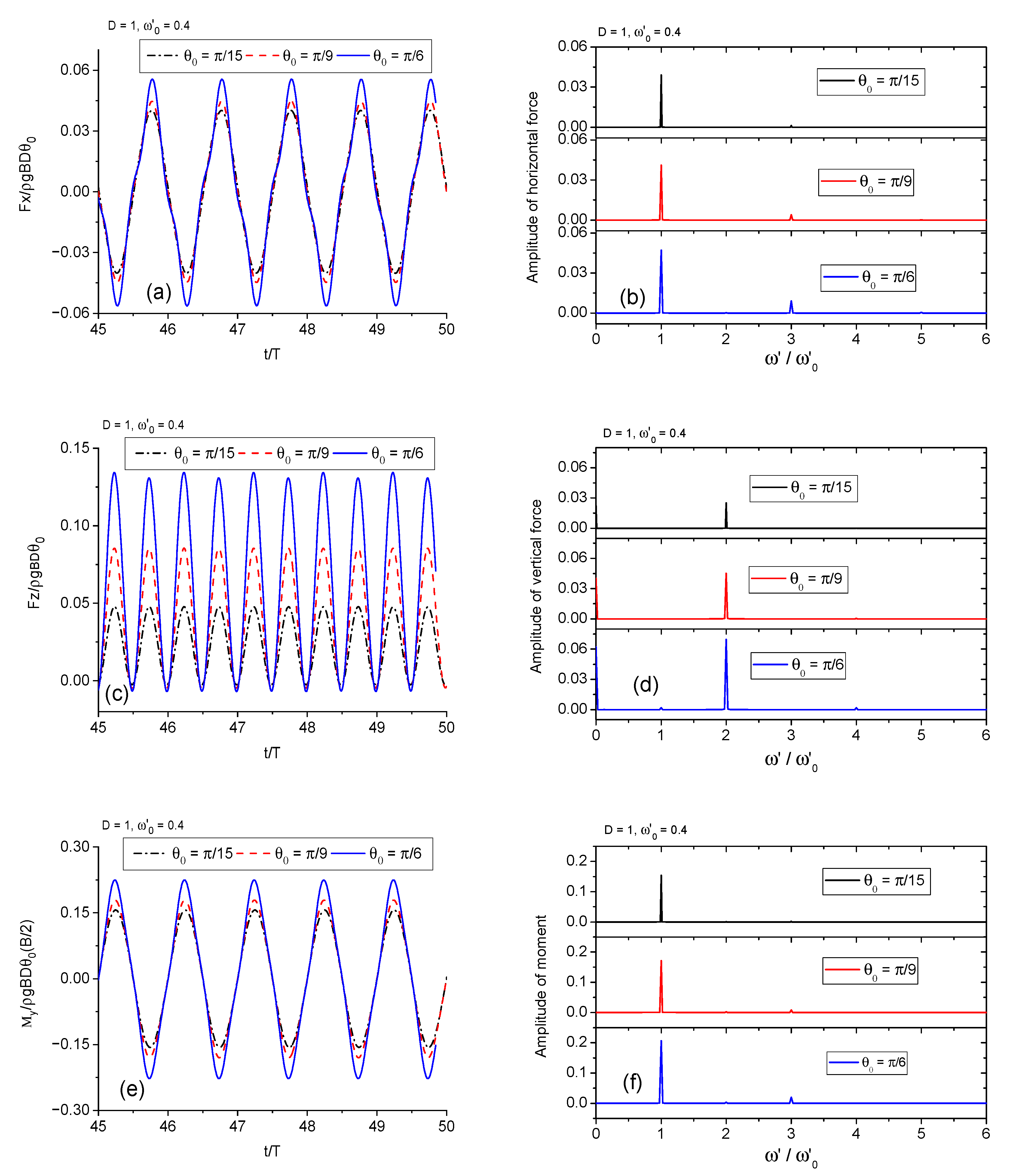
Figure 15.
FFT analysis of normalized forces and moments when , : (a) FFT analysis of horizontal forces; (b) FFT analysis of vertical forces; (c) FFT analysis of moment.
Figure 15.
FFT analysis of normalized forces and moments when , : (a) FFT analysis of horizontal forces; (b) FFT analysis of vertical forces; (c) FFT analysis of moment.

Figure 16.
Comparisons of combined motion with those of single-mode motion when : (a,b) horizontal force comparison with sway motion; (c,d) vertical force comparison with heave motion; (e,f) moment comparison with roll motion.
Figure 16.
Comparisons of combined motion with those of single-mode motion when : (a,b) horizontal force comparison with sway motion; (c,d) vertical force comparison with heave motion; (e,f) moment comparison with roll motion.
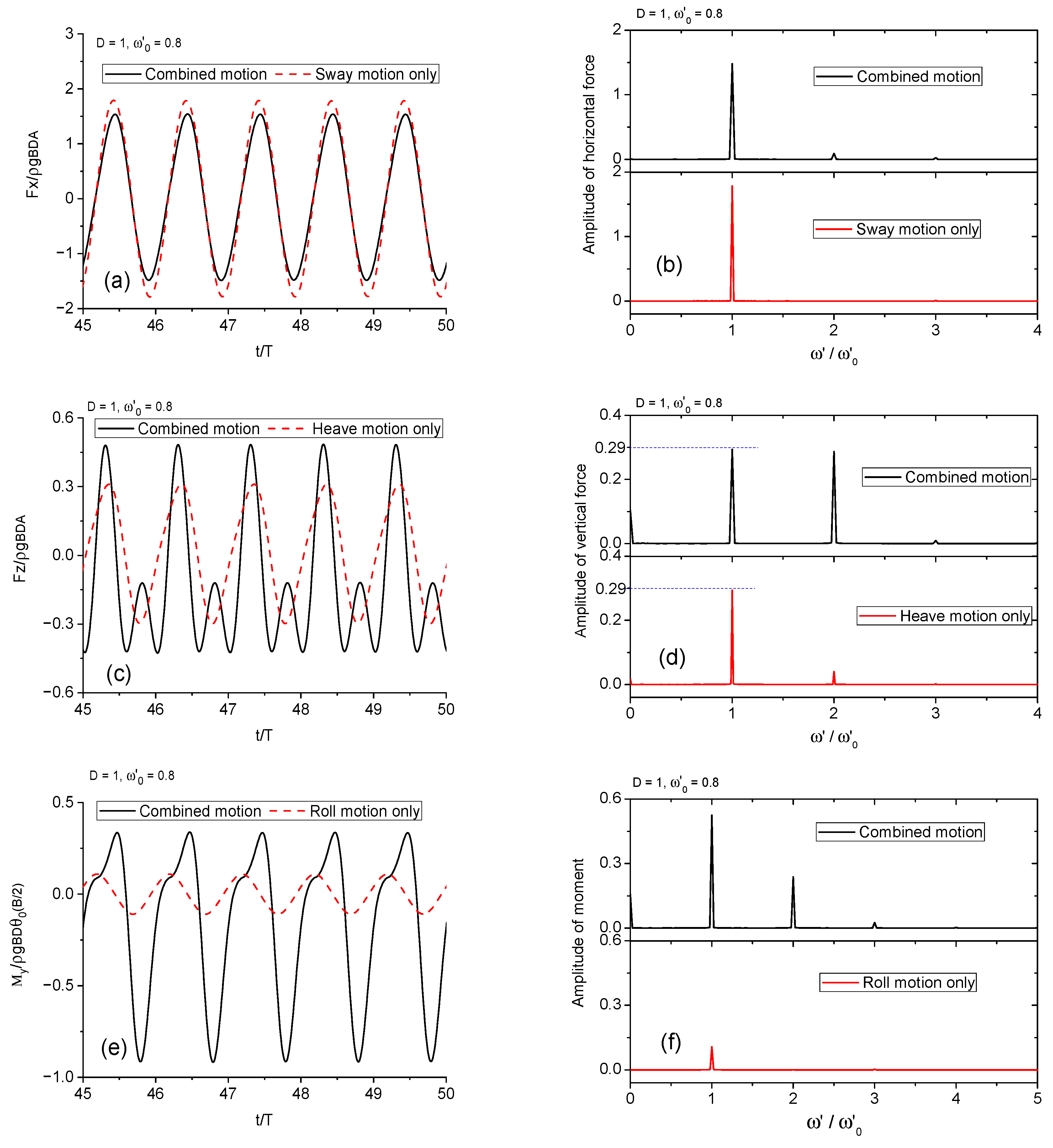
Figure 17.
Development of free surface profile for the body under combined motion when .
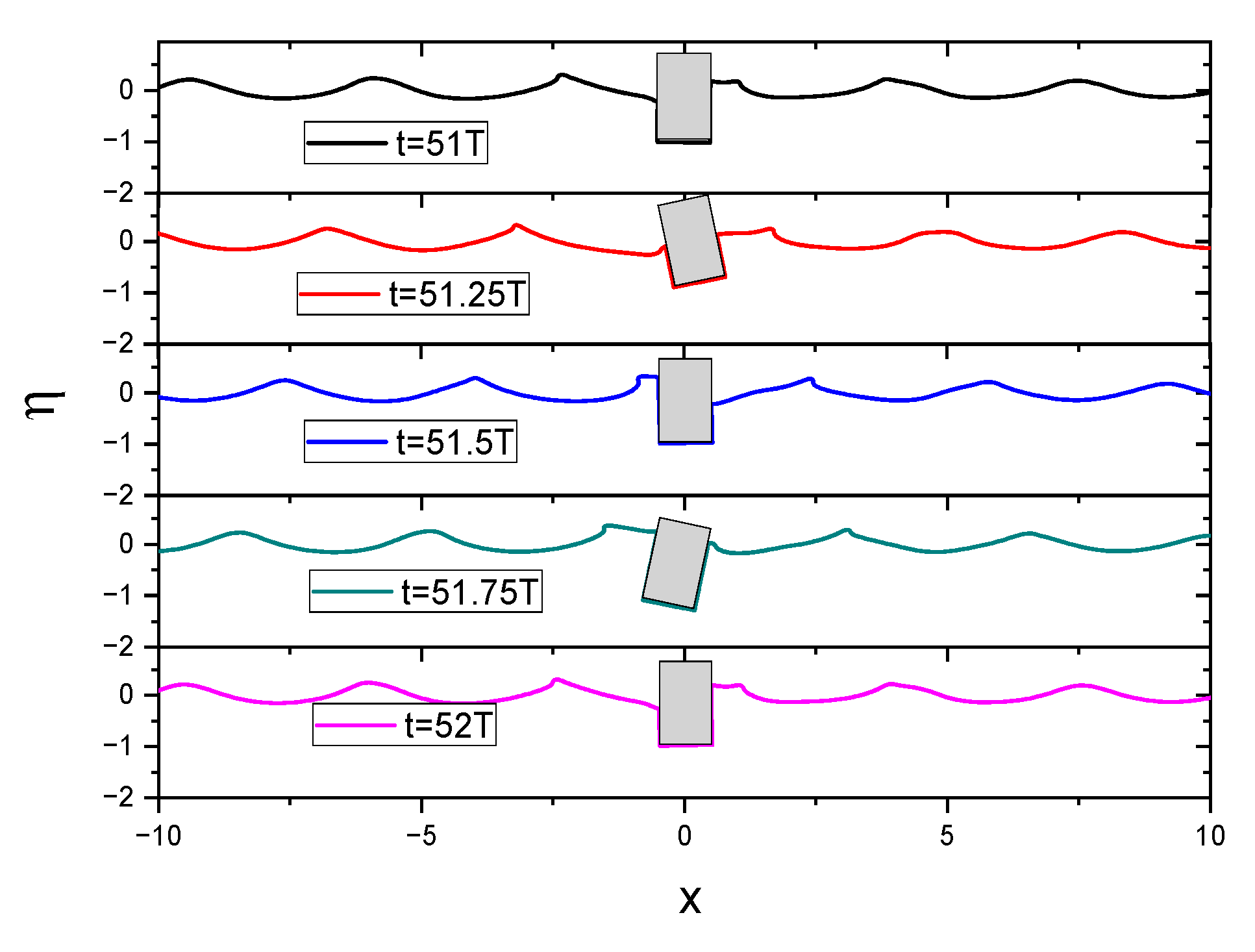
Figure 18.
Comparisons of combined motion with those of single-mode motion when : (a,b) horizontal force comparison with sway motion; (c,d) vertical force comparison with heave motion; (e,f) moment comparison with roll motion.
Figure 18.
Comparisons of combined motion with those of single-mode motion when : (a,b) horizontal force comparison with sway motion; (c,d) vertical force comparison with heave motion; (e,f) moment comparison with roll motion.
Publisher’s Note: MDPI stays neutral with regard to jurisdictional claims in published maps and institutional affiliations. |
© 2020 by the authors. Licensee MDPI, Basel, Switzerland. This article is an open access article distributed under the terms and conditions of the Creative Commons Attribution (CC BY) license (http://creativecommons.org/licenses/by/4.0/).
Share and Cite
MDPI and ACS Style
Li, Y.; Long, Y. Numerical Study on Wave Radiation by a Barge with Large Amplitudes and Frequencies. J. Mar. Sci. Eng. 2020, 8, 1034. https://doi.org/10.3390/jmse8121034
AMA Style
Li Y, Long Y. Numerical Study on Wave Radiation by a Barge with Large Amplitudes and Frequencies. Journal of Marine Science and Engineering. 2020; 8(12):1034. https://doi.org/10.3390/jmse8121034
Chicago/Turabian StyleLi, Yajie, and Yun Long. 2020. "Numerical Study on Wave Radiation by a Barge with Large Amplitudes and Frequencies" Journal of Marine Science and Engineering 8, no. 12: 1034. https://doi.org/10.3390/jmse8121034
Note that from the first issue of 2016, this journal uses article numbers instead of page numbers. See further details here.