Evaluation of the Viscous Drag for a Domed Cylindrical Moored Wave Energy Converter


Centre for Marine and Renewable Energy (MaREI), University College Cork, T12 Cork, Ireland
*
Author to whom correspondence should be addressed.
J. Mar. Sci. Eng. 2019, 7(4), 120; https://doi.org/10.3390/jmse7040120
Submission received: 14 March 2019
/
Revised: 11 April 2019
/
Accepted: 16 April 2019
/
Published: 25 April 2019
(This article belongs to the Special Issue Nonlinear Numerical Modelling of Wave Energy Converters)
Abstract
:Viscous drag, nonlinear in nature, is an important aspect of the fluid–structure interaction modelling and is usually not taken into account when the fluid is assumed to be inviscid. Potential flow solvers can competently compute radiation damping, which is related to the radiated wave field. However, the drag damping primarily related to the viscous effects is usually neglected in the radiation/diffraction problems solved by the boundary element method (BEM), also known as the boundary integral element method (BIEM). This drag force can have a significant impact in the case of structures extending much deeper below the free surface, or for those that are completely submerged. In this paper, the drag coefficient was quantified for the heave and surge response of a structure which consists of a moored horizontally oriented domed cylinder with two surface piercing square columns located at the top surface. The domed cylinder is the primary part and is submerged. The drag coefficient is estimated using the experimental measurements related to harmonic monochromatic wave–structure interaction. Finally, this estimated drag coefficient was used in the modified time domain model, which includes the nonlinear viscous correction term, and the resulting device response in heave and surge directions is presented for an irregular incoming wave field. The comparison of the numerical model and the experiments validates the estimated values obtained earlier. Prior to the time domain model, frequency-dependent parameters such as added mass, radiation damping, and excitation force were computed using three mainstream potential flow packages (that is, ANSYS AQWA, WAMIT, and NEMOH), and a comparison is presented. The effect of free surface on the drag coefficient is investigated through differences in values between heave and surge modes.
1. Introduction and Background
A part of the resistance to structures moving in fluid, for example, marine energy devices, is caused by the fluid viscosity. Displaced structures set up waves and generate eddies. Resistance due to waves is sometimes termed as gravity resistance as the waves build up potential energy. However, eddy formation and their resistance (or dissipation) is more related to the viscosity of the fluid. Therefore, fully submerged structures (such as submarines) experience relatively significant viscous resistance, while the generated waves and eddies ultimately dissipate due to the viscosity of the fluid.
The seakeeping and/or manoeuvring time domain mathematical model [1] relies on the frequency domain hydrodynamic parameters, which are computed through linear potential theory, where fluid is assumed nonviscous (inviscid).
Inviscid potential flow solvers provide robust solution of the wave–structure interaction response for a wave energy device and in order to account for the viscous effects, the use of the Morison equation has been reported by a number of studies [2,3,4]. However, identification of the drag coefficient used in this approach is quite challenging. A value for this coefficient can be found empirically or using numerical modelling, such as the RANS (Reynolds-averaged Navier–Stokes) solvers [5,6,7,8,9].
The authors of [10] examined two-dimensional nonlinear time-domain solutions of the viscous effects for a twin rectangular hull under heave oscillation and compared results with existing linear, inviscid frequency domain data. In the case for low frequencies, the viscous effects are reported to be significant even for small amplitudes of the body oscillation. Estimate of viscous effects is crucial for an accurate numerical modelling of the wave energy structures. In order to include the nonlinear drag force in such numerical modelling, the CFD (computational fluid dynamics) solvers can be employed to deduce the additional damping coefficients for a floating wave energy structure. In Reference [8], the viscous damping of a three-dimensional model of the float-over barge was estimated using a RANS (Reynolds-averaged Navier–Stokes) solver and a comparison with the experimental data showed applicability of the CFD for evaluation of the viscous damping associated with the low frequency waves.
The viscous drag’s impact on the power production of a generic surging type wave energy converter was studied using a nonlinear time domain model with viscous correction [2,7]. In relation to the viscous drag, the power output for a heaving wave energy converter was analysed in Reference [6], where it was reported that the viscous drag force caused a 4% reduction in the annual power production of such a point absorber device. A similar study for a generic surging type wave energy converter reported that the numerical power prediction can result in significant overestimation (more than 100%) if viscous effects are not taken into account [2]. CFD simulations can provide drag values (coefficient) that can be used in the time domain dynamic numerical model, as reported by References [6,7,11].
In addition to the viscous drag, the incoming wave nonlinearity, moorings scopes, and the power take off offer added nonlinear contributions, as has been reviewed in Reference [3]. In Reference [4], CFD modelling of the viscous effects was reported for a generic model scale buoy moored in waves, and issues and limitations associated with the CFD analysis were also discussed, such as being computationally demanding for long term power prediction. Recently, the authors of [12] reported a study of the nonlinear forces on a cylindrical generic moored point-absorbing wave energy converter using a RANS solver, the Euler equations solution, and the linear radiation–diffraction method. Viscous effects in relation to device scale are discussed. The scale effects and viscous drag relationship is usually seen as drag verses Reynolds number problem; however, for oscillatory flow, this can be a challenging task, in particular when RANS solvers are used, because results can be very sensitive to the mesh structure and the turbulence model used. The viscous force can have a significant impact on the control strategy considered. For a heaving wave follower type wave energy device, the identification of the drag using an extended Kalman filter was reported in Reference [13]; the study showed the importance of the viscous correction in relation to the control system performance.
In relation to multidegree of freedom motion, in Reference [14], the heading stability of a turret-moored ship was assessed by varying damping in different modes of motion. The study showed that viscous effects in pitch mode are stronger than heave or roll. However, for wave energy converters, there is a need to investigate the variation of the drag coefficient in relation to the multidegree of freedom response. In this paper, the drag coefficient was estimated for a moored wave energy converter, and a comparison of the nonlinear time domain numerical model against experimental data is presented. This study shows that small-scale monochromatic tests data can be used to identify the drag coefficient needed for the Morison equation’s nonlinear viscous term. Further, this paper shows that for a device that has an irregular shape, there can be considerable difference in the identified drag coefficient in relation to the motion mode (such as heave and surge response).
2. Methodology
2.1. Introduction
The significance of the viscous drag part of the hydrodynamic interaction that a marine structure experiences is case-dependent, due to a varying encounter (wave) frequency and the response amplitudes, which are usually classified in the form of the Reynolds number (Re) and the Keulegan–Carpenter (KC) number (Equation (2)). By definition, Re is given by Equation (1), where the numerator is the inertial part and the denominator is the viscous contribution:
where,
- –
- = fluid density,
- –
- U = maximum velocity,
- –
- D = relevant characteristic dimension of the rigid structure,
- –
- = dynamic viscosity of the fluid.
For the oscillatory flow phenomenon, the problem becomes more complex as the drag force also depends on another nondimensional measure of the KC number (for example, see [15]):
with:
- –
- = amplitude of the sinusoidal velocity,
- –
- T = time period of the sinusoidal velocity.
For sinusoidal motion ( or for deep water waves), the KC number can be rewritten as ([15]):
where a is the amplitude of the wave or of structure displacement.
The viscous drag force evaluation for simple geometrical shapes like cylinders and/or squares (with smooth and sharp corners) has been widely studied.
The viscous parameter is defined as the ratio of Re to the KC number. The amplitude of oscillation and the structures geometry are the relevant properties that quantify the viscous force in a particular situation.
Marine renewable devices such as wave energy converters are designed to exhibit relatively much larger motion amplitudes compared to conventional tension leg platforms (TLPs). Therefore, viscous effects are of primary importance, as their influence will have a direct effect on the energy production. Preliminary design assessment of such devices has implemented the seakeeping mathematical models where the viscous force (due to skin friction, flow separation, and eddies contribution) can be included using an additional viscous drag term [1,16]. As viscous force incorporation in this paper is achieved through the Morison equation, therefore, a brief introduction of the Morison equation is presented next.
The Morison equation ([17]) provides a semi-empirical formulation to model the unsteady force on rigid structures in oscillatory flow. According to this expression, the total in-line force on an immersed object within an oscillatory viscous fluid with velocity and acceleration is expressed as a summation of two components:
- –
- force due to the inertia; an effect of the irrotational (potential) assumption, i.e., ;
- –
- force due to the viscous drag; effect of the skin friction and flow separation, i.e.,
For a three-dimensional structure moving in-line with the oscillatory flow, the Morison equation becomes [15]:
where t is the time index and:
| = fluid density, | = relevant cross-sectional area, | ||
| V | = volume of the structure, | = drag coefficient, | |
| = inertia coefficient, | = fluid velocity, | ||
| = fluid acceleration, | U | = body velocity, | |
| = body acceleration. |
The last term () represents the Froude–Krylov force. The inertial force proposed by the Morison equation is proportional to the acceleration of the flow, whereas the viscous drag part is proportional to the time-dependent flow velocity and acts in the direction of the velocity. For a fixed structure in oscillatory flow, the inertia coefficient becomes .
The device is composed of two primary parts:
- (i).
- a submerged horizontal cylindrical part which has domed ends;
- (ii).
- two rectangular columns attached at the top surface of the domed cylinder.
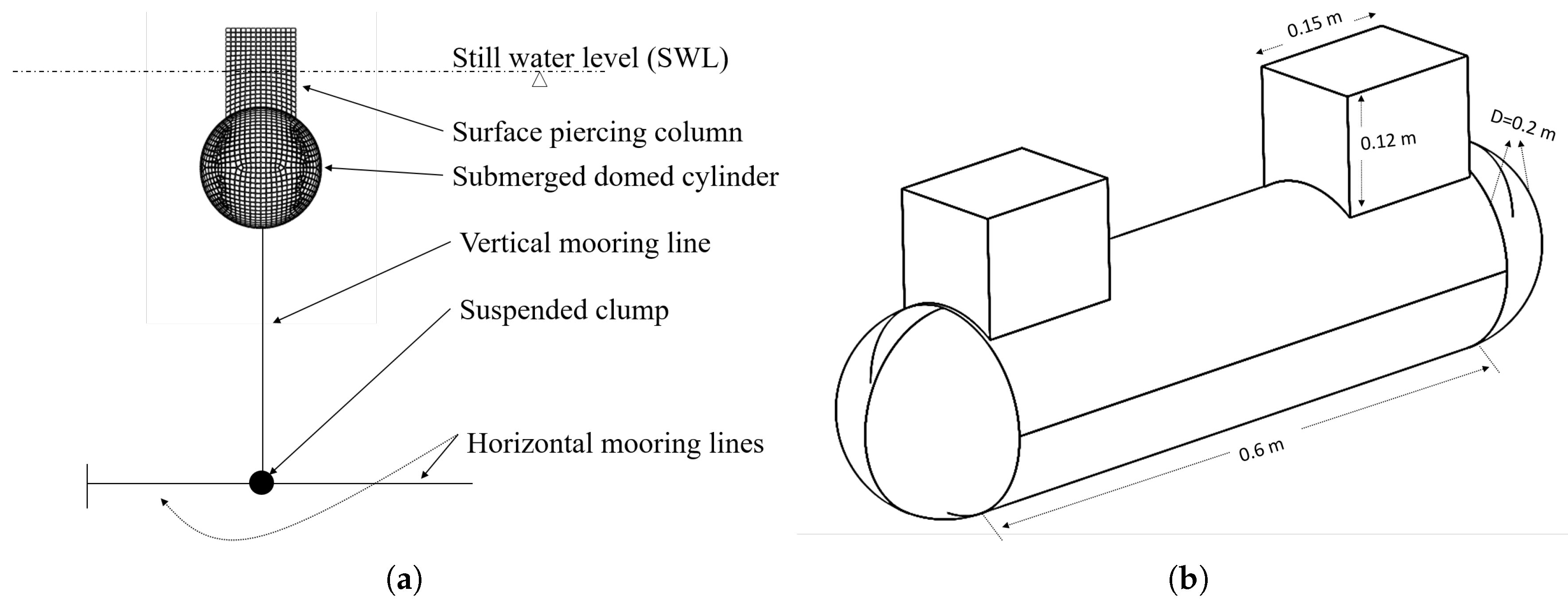
The rectangular columns are in surface piercing mode, and the draft depth is such that only half the length of these columns is submerged. The device is moored using two vertical mooring lines attached to the submerged cylinder and a free floating clump mass. The clump mass is then connected to the bottom (floor) of the tank using two additional horizontal mooring lines. For visual description of this setup, a picture of the meshed geometry and the schematic showing device dimensions are presented in Figure 1.
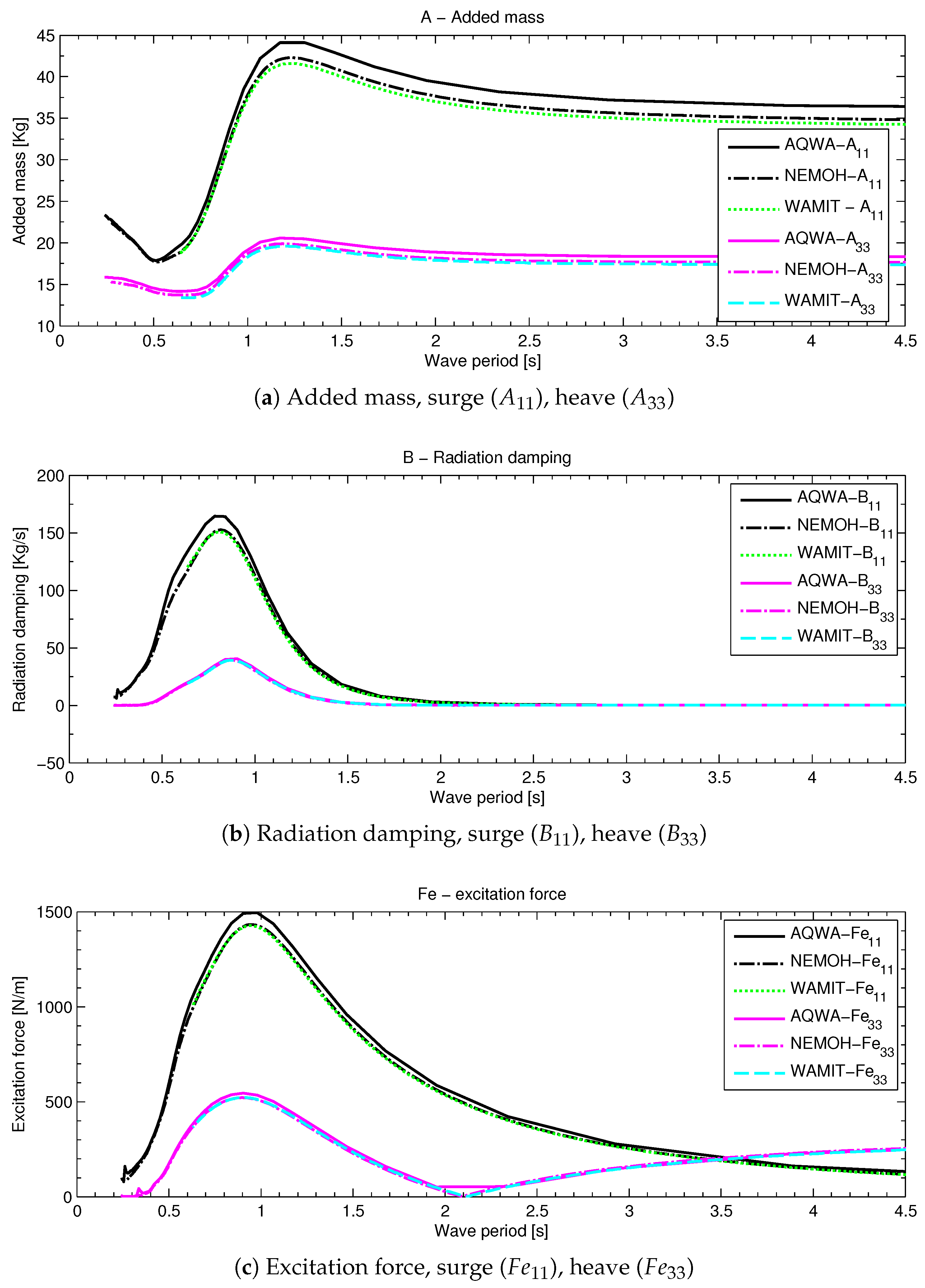
Frequency-dependent hydrodynamic properties are computed using a radiation–diffraction boundary element method solver. Three state of the art solvers—WAMIT (Software package of WAMIT Inc. (http://www.wamit.com/)), NEMOH (Open source code from LHEEA lab, Ecole Centrale de Nantes, France, version 2.0.) and AQWA (Software product of ANSYS Inc. (http://www.ansys.com/) version14.5.))—were employed for this purpose, and a comparison of these packages is then reported. NEMOH is an open source code that is based on Aquaplus, which is a BEM solver for calculation of first-order hydrodynamic coefficients.
Utilising the frequency domain data of NEMOH, a time domain model was used to compute the time series response of the floating structure, and the results are then compared against the experimental measurements. The body geometry and input parameters, such as mass properties, stiffness, and damping, are sourced from the panchromatic wave tests for configuration B of Reference [18] (see Figure 1), and these parameters are shown in Table 2. The time domain solution was derived using the convolution integral for the radiation force according to Cummins relation [19], and the viscous drag of the fluid structure interaction is included in the time domain model using nonlinear quadratic drag damping of Morison’s equation [17]. Following NEMOH’s results, a time domain model with viscous correction ([2]) was then implemented. In Reference [2] such a model was referred to as a potential time domain viscous (PTDV) model, and a comparison of the viscous correction was presented against CFD computations. It was shown that for a floating wave energy converter, viscous contributions show a significant impact on the power output of the surging wave energy device. Only surge mode was reported in that study with values derived from curve fitting of the Morison equation and the radiation force using CFD [7].
However, in the study presented here, the structure is a small-scale model which is composed of a submerged and a semisubmerged part, and the experimental measurements data were used for the estimate of the values.
2.2. Frequency Domain Model And Results
Hydrodynamic parameters from frequency domain analysis using WAMIT, AQWA, and NEMOH were computed using a slightly varying mesh structure and a number of tested frequency points. These frequency domain results of the hydrodynamic parameters are shown in Figure 2a–c. Compared to RANSE solvers, mesh independence for BEM solvers of the potential theory is relatively usually not an issue unless the considered panels are extremely coarse [2]. In the modelling reported here, it was ensured that a fairly dense mesh had been achieved, for example, in NEMOH and AQWA, the body was discretised into 1629 panels. It can be seen that results from all three packages are in reasonably good agreement; however, a small (negligible) percentage of the discrepancy in these results can be attributed to the differences of mesh structures, input frequency points, and the computational resource. Furthermore, the range of the frequency steps used in this computation is considerably large for NEMOH (300 frequency steps) and WAMIT (300 frequency steps) compared to the AQWA, where only 50 frequencies were used.
In Figure 2a, it can be seen that the added mass due to surge motion is approximately twice the added mass associated with the heave motion. This shows that the mass of the water that is accelerated due to surge motion of the structure is much higher (nearly twice) compared to the heave motion. Similar, from Figure 2b, radiation damping experienced by the structure due to radiated wave field is also considerably higher compared to the one observed in heave motion. This shows that the rigid floating structure is radiating significantly more waves due to surge motion compared to the heave motion. However, for waves with a wave period higher than 1.8 s (i.e., frequency lower than 3.5 rad/s), the radiation damping drops to zero for both of the cases, i.e., the surge and the heave. It can be seen in Figure 2c that the magnitude of the complex amplitude of the wave excitation force component in surge direction is significantly higher than the corresponding component in the heave direction.
Following the computation of the frequency-dependent hydrodynamic parameters (such as added mass matrix A, radiation damping matrix B, and the excitation force vector ), the frequency domain response amplitude of the device is obtained from the complex magnitude of using Equation (5):
where:
| = angular frequency in [rad/s], | m | = mass of the structure, | |
| = frequency-dependent added mass, | = frequency-dependent wave damping, | ||
| C | = linear viscous damping (if any), | = hydrostatic stiffness, | |
| K | = additional stiffness (if any), | = frequency-dependent excitation force amplitude | |
| (complex variable). |
The magnitude of the is the response amplitude operator (RAO) as a function of the wave-frequency of unit wave-amplitude. C is the additional linear damping. For frequency domain analysis, a value for this linear damping was adopted from free decay tests of surge and heave motions shown in Reference [18] (Figure 7). A value of 3 N/m/s for heave and 7 N/m/s for the surge motion were used for the linear frequency domain results.
2.3. Time Domain Model
Time domain analysis (based on frequency domain parameters of NEMOH) relies on the equation of motion Equation (6):
where:
- –
- = added mass at infinite frequency,
- –
- = acceleration of structure,
- –
- = wave excitation force,
- –
- = non-linear viscous drag force.
Representation of the term in a state–space model is given below, in Equation (7):
where:
- –
- = complex velocity-dependent variables,
- –
- = real part of the Prony coefficient,
- –
- = imaginary part of the Prony coefficient.
In Equation (6), is the additional quadratic drag damping term in accordance with the Morison equation. i.e.,:
where is the relative velocity, with being the instantaneous velocity of the incident wave. is the body velocity. is the fluid density. is the relevant cross-sectional area of the structure. The excitation force due to irregular wave signal is given by:
where ℜ denotes the real part of the complex variable, and:
- –
- = wave amplitude of frequency wave,
- –
- = frequency-dependent wave excitation force (complex variable),
- –
- = phase variable used to generate random wave field’
- –
- = total number of wave frequencies.
Here (in Equation (6)), the convolution product of radiation impulse response function times the velocity has been replaced by additional state variable using the approach described in Reference [20]. The use of the prony method is implied for the computation of coefficients and using the method shown in Reference [21]. In Equation (7), is the total number of prony coefficients. Finally, the equation of motion (Equation (6)) is solved using the ode45 (based on an explicit Runge–Kutta formula) solver function in MATLAB.
2.4. Evaluation of the Drag Coefficient ()
The drag coefficient of the Morison equation (Equation (4)) can be determined by means of experiments or numerical computations. The process involves measurements/computations of the force time history from the experiments or numerical computations. This force series is then utilised in the curve fitting against the Morison equation yielding appropriate coefficient values based on the criteria of the curve fitting approach. For such a purpose, a number of methods can be considered, for example [22]: Morison’s method, the Fourier series approach, least squares method, and weighted least squares method.
For the present case study, the experimental normalised motion response, as reported in Reference [18], was used in order to estimate the values, and this was achieved by curve fitting of these experimental readings against the time domain model of Equation (6) through the least squares approach.
The Morison viscous force term is proportional to the cross-sectional area of the moving structure. From the geometry of the structure (Figure 1), it can be seen that this area in heave mode is the cross-sectional area of the domed cylinder orthogonal to the heave direction; however, for the surge mode, the cylindrical cross-sectional area orthogonal to the surge direction has an additional contribution from the two individual surface-piercing rectangular columns.
3. Results
3.1. The Drag Coefficient ()
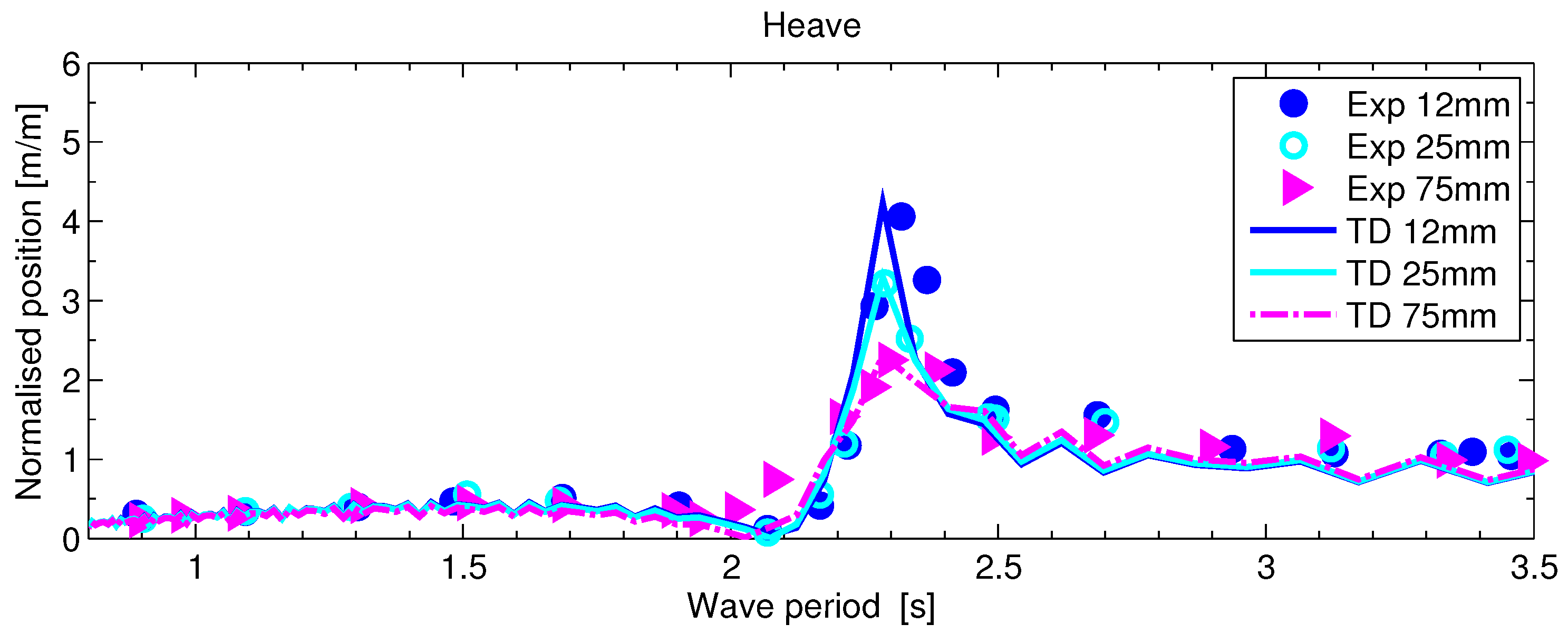
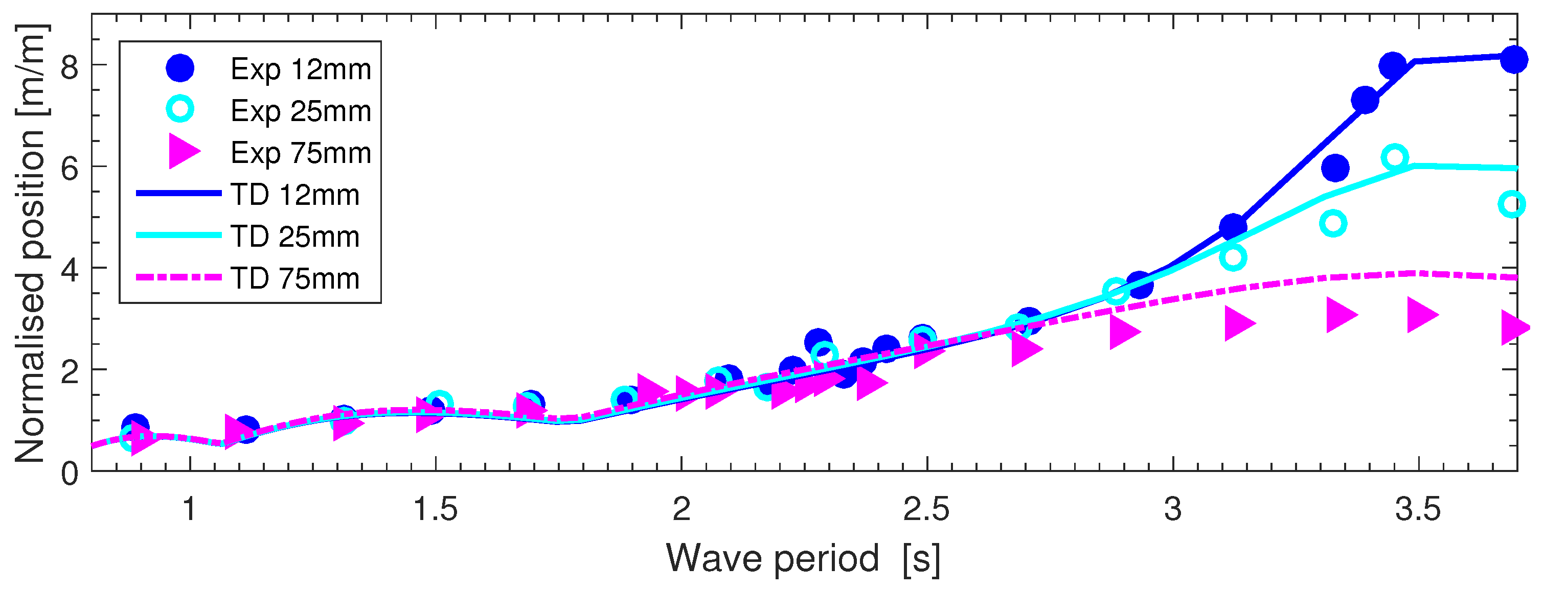
In Figure 3, normalised heave–response is shown against experiments for the estimated value of 0.5, whereas for surge–response, a similar comparison is shown in Figure 4, where the estimated value is 2.4.
Corresponding KC and Re values can be computed using Equations (3) and (1). For the KC number, the amplitude of motion a is obtained through multiplication of the experimental values of the normalised response (say ) per unit wave amplitude (shown in Figure 3 and Figure 4) by the corresponding wave amplitude. Considering the sinusoidal response, for the Re number, the velocity amplitude U can be obtained by the following relation (Equation (10)):
where is the wave frequency in . The KC and Re values are shown in Table 1.
3.2. Time Domain Model Results And Analysis
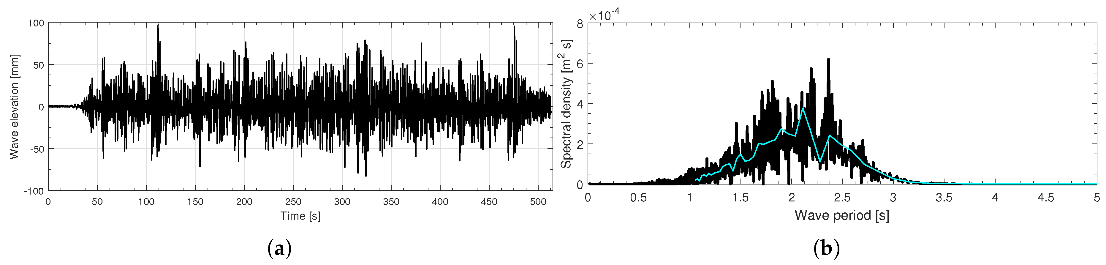
The instantaneous time history of the heave and surge displacement for the given irregular random wave time series are computed using the time domain model. The time series and the corresponding spectral plot of the incoming wave is shown in Figure 5; the peak period of the random wave is approximately 2.3 s, and the significant wave height is ≈72.6 mm. It can be seen that the the resonance period of the device was within the range of the considered wave spectrum.
Time taken for each time domain computation for the given wave time series of 512 s with time step of 0.00729 s was 2.28 min. Input parameters for all case studies are shown in Table 2. Key properties in this Table 2 are the total stiffness contributions experienced by the float due to attached mooring lines [18].
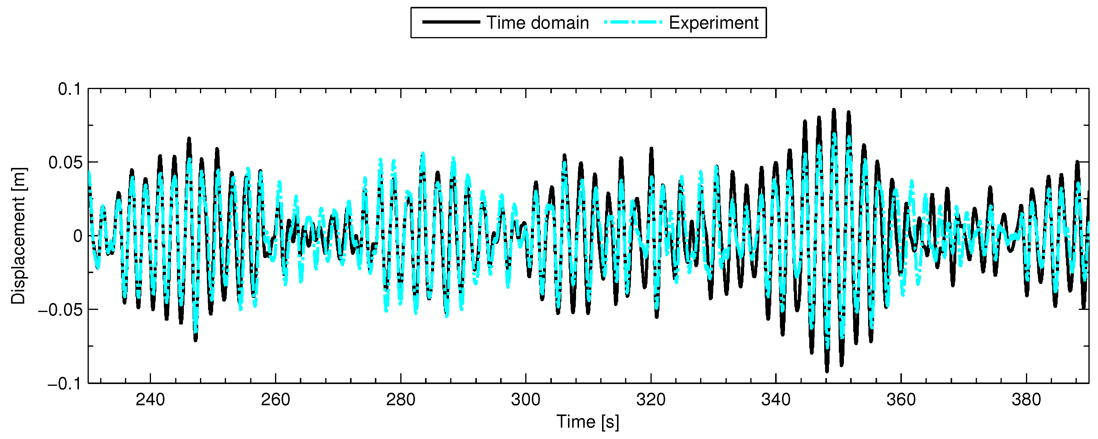
For the heave mode response, an extract of the time series results from Equation (6) are shown against the measured heave response in Figure 6. A similar comparison for the surge case is shown in Figure 7. The root mean squared error (RMSE) of the computed and experimental results can be computed using Equation (11). RMSE values of time series results are shown in Table 3.
Here, refers to the computational results and to the experimental measurements, j and N are the index and the total number of data points, respectively.
A comparison between the experiment data and the computed response using the time domain model (Equation (6)) was also done in terms of the spectral densities. For this, the frequency components of the fast Fourier transform were used to obtain the spectral density using Equation (12). In order to eliminate the initial conditions influence, from the 512s of time series data, results from 256 s onward were used for this analysis.
where y is the fast Fourier transform of the input signal, is the complex conjugate of y, N is the number of data points, and the sampling time. The corresponding frequency in this case is given by Equation (13):
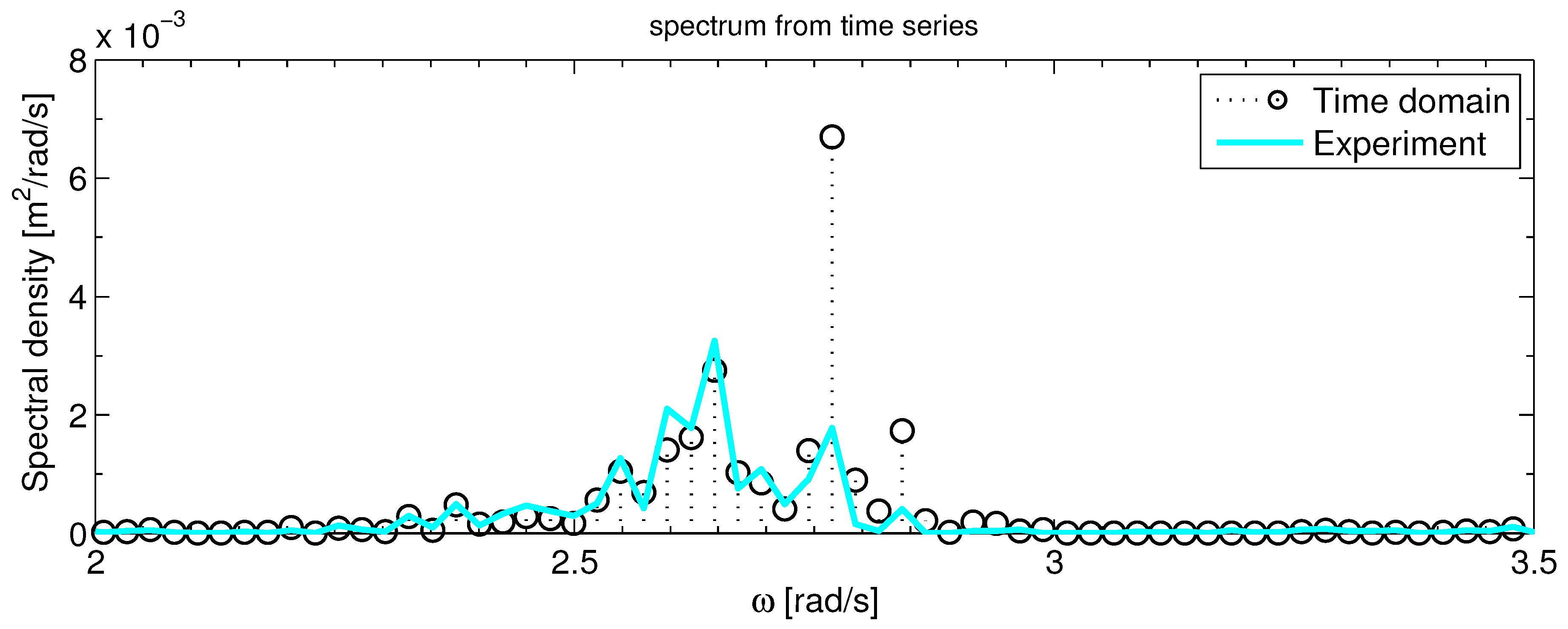
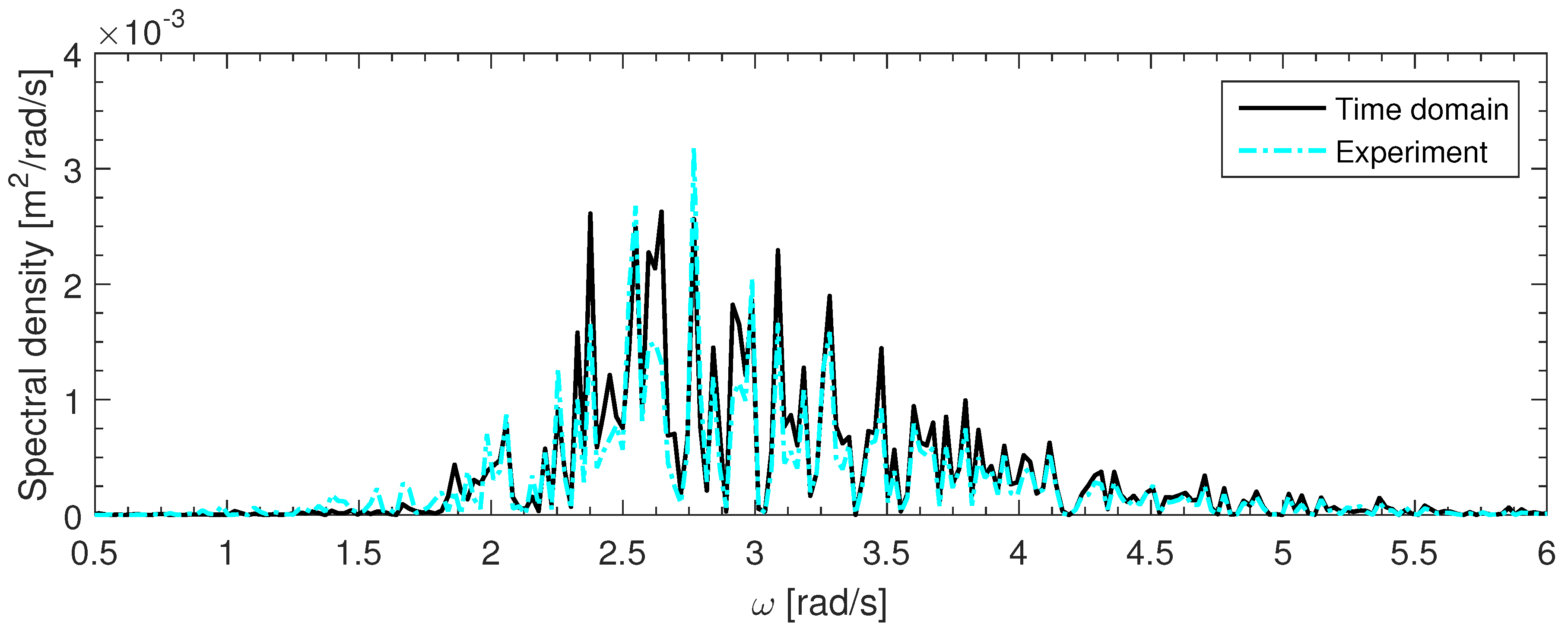
The spectral density of heave is shown in Figure 8, where the results show a good match with the experiment; however, it can be seen that the time domain model carries some overprediction, which is shown at two frequency points. For the surge case, the spectral density is presented in Figure 9. Again, it is seen that time domain model response, although in good level of accuracy, still carries some minor overprediction, as is shown by some spikes at a few frequencies.
From the irregular wave response, the RAO or normalised response RN shown in Figure 10 and Figure 11 was obtained via Equation (14):
- –
- = Spectral density of the response,
- –
- = Spectral density of the wave signal.
Figure 10 shows the heave response of the device in relation to the unit wave amplitude at various wave periods. Here, experiments from the regular wave of varying amplitudes are plotted alongside computational results of the frequency and time domain analysis using NEMOH’s hydrodynamic parameters. For this graph, the resulting response is divided by the wave amplitude in order to produce the normalised position. Figure 11 shows the frequency domain response amplitude of the surge motion of the device alongside the normalised response from the panchromatic waves and measured data from experiments for monochromatic waves of fixed amplitudes. It is seen that the device response to the panchromatic wave force signal is in accordance with the trend predicted by the frequency domain approach and the experiments.
The RMSE of the time history responses (surge and heave) is shown in Table 3.
3.3. Discussion
Following the RMSE shown in Table 3, it is noted that incorporation of the viscous force produced very good agreement with the experiments; however, the heave response of the device is relatively in better agreement with the experiments compared to the surge response’s RMSE. From analysis of the spectral curves shown in Figure 8 and Figure 9, it can be noted that for the surge case, experimental results carry significant contributions for frequencies below 2.5 rad/s as well as for frequencies above 3.5 rad/s compared to the heave case (Figure 8).
For a measure of correlation between two signals (or series) (namely and , for i = 1,2,3,...,n), the correlation coefficient r can be computed using Equation (15):
where and are the mean values of x and y, respectively, and n is the total number of data points. The value of the correlation coefficient between the prediction and the experimental data is shown in Table 4. As the value of this correlation coefficient is above 0.9, this shows that the results are in excellent agreement.
From Figure 10 and Figure 11, it is worth noticing that the frequency domain approach is the most robust and offered a fairly good indication of the float’s response to waves of differing frequencies per unit wave amplitude. Overall, a normalised position from the panchromatic wave field showed a quite similar trend to that of the linear frequency domain results; however, there are instances where nonlinear drag force became significant.
It can be seen that the viscous correction in the time domain model—which is based on linear frequency domain data—offered a robust method compared to more rigorous computational methods, such as Reynolds-averaged Navier–Stokes equations (RANSE) models, where computation of a monochromatic wave requires a relatively much longer computation time; however, for the quantification of the viscous drag coefficients and for the validation of the modified time domain models, CFD can be employed, as has been demonstrated [23].
One important feature observed in this modelling is the magnitude of the drag coefficient for the surge and heave motions. As shown in Table 2, the drag coefficient obtained for the heave motion is nearly 50% less than surge motion. This implies that the significance of the drag force for heave is considerably less compared to that of the surge case. The cross-sectional area or the water-plane area for the surge mode is larger than that for the heave mode due to, firstly, the additional rectangular columns and, secondly, the fact that the device is surface piercing and a part of the extra damping is, possibly, coming from the nonlinearity of the free surface interaction.
For heave motion, because the surface-piercing profile, as part of the device, is above the water plane and there is no motion against the direction of the incoming waves, there is relatively less drag offered by the free surface interaction. Furthermore, a much higher total stiffness (hydrostatic plus moorings) force can counteract part of the drag force in heave mode; hence, the resultant drag damping value is less than surge.
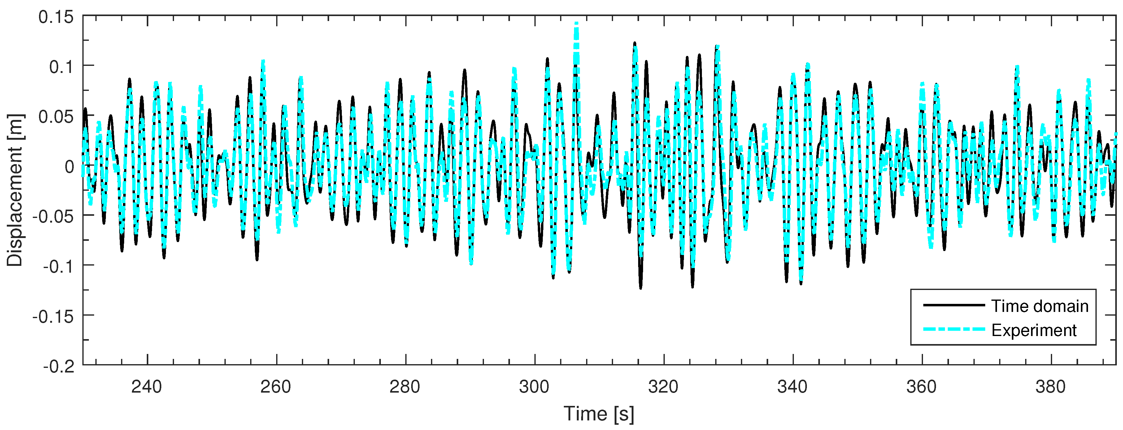
Finally, an analysis of the time domain model with and without an additional nonlinear viscous force () is presented. An extract of the time series response is shown in Figure 12. The case with refers to the scenario where is not included in the model. It is observed that in the absence of the additional drag force, the RMSE value (corresponding to the experiment measurements) for the heave case (where instead of nonlinear damping term, the linear damping, similar to the frequency domain model, of 3 was employed in order to avoid unrealistic motion amplification) increases by 38%. Similarly, for , the surge response RMSE value increases by 22.6%. This shows the relative importance of the nonlinear features that can be competently captured using drag force .
4. Conclusions
It was demonstrated in this paper that results for the frequency domain parameters computed using three radiation–diffraction panel codes—WAMIT, AQWA and NEMOH—show very good agreement.
Simulations for an irregular (panchromatic) wave were performed using the nonlinear time domain model, and a comparison against the experimental results was presented. The statistical measures, such as RMSE and correlation coefficient of the computed and the experimental data, were reported, which demonstrated a very good agreement. Thus, nonlinear features of wave structure interactions can be taken into account through the additional nonlinear viscous drag damping in accordance with the Morison equation.
Preliminary hydrodynamic evaluation using the frequency domain linear approach was shown to be reasonably accurate, and this produced a robust estimate of the structure’s response for a range of wave frequencies. However, from the normalised response of time series results shown against the RAO of the linear frequency domain model, it was observed that there are instances where the nonlinear viscous effects were significant. Consequently, it is concluded that viscous effects can cause a considerable influence on the resultant response.
For the particular device, it was shown that the magnitude of the estimated drag coefficient for the heave motion is ≈5 times less than the corresponding value of the surge motion.
Author Contributions
Investigation and numerical modelling, M.A.B.; Validation, J.M.; Writing—original draft, M.A.B.; Writing—review and editing, M.A.B. and J.M.
Funding
This research was funded by Science Foundation Ireland (SFI) funding of MaREI.
Acknowledgments
The authors like to thank Centre for Ocean Energy Research (COER), Maynooth, for providing the experimental data. The authors would like to thank Wanan Sheng for his valuable comments and discussions during the validation of this work.
Conflicts of Interest
The authors declare no conflict of interest.
References
- Perez, T. Ship Motion Control: Course Keeping and Roll Stabilisation Using Rudder and Fins; Springer: Berlin/Heidelberg, Germany, 2005. [Google Scholar]
- Bhinder, M.A.; Babarit, A.; Gentaz, L.; Ferrant, P. Potential time domain model with viscous correction and CFD analysis of a generic surging floating wave energy converter. Int. J. Mar. Energy 2015, 10, 70–96. [Google Scholar] [CrossRef]
- Penalba, M.; Giorgi, G.; Ringwood, J. A Review of Non-Linear Approaches for Wave Energy Converter Modelling. In Proceedings of the 11th European Wave and Tidal Energy Conference, Nantes, France, 6–11 September 2015. [Google Scholar]
- Palm, J.; Eskilsson, C.; Paredes, G.M.; Bergdahl, L. Coupled mooring analysis for floating wave energy converters using CFD: Formulation and validation. Int. J. Mar. Energy 2016, 16, 83–99. [Google Scholar] [CrossRef]
- Thilleul, O.; Babarit, A.; Drouet, A.; Le Floch, S. Validation of CFD for the determination of damping coefficients for the use of Wave Energy Converters modelling. In Proceedings of the International Conference on Offshore Mechanics and Arctic Engineering-OMAE, Nantes, France, 9–14 June 2013; Volume 9. [Google Scholar] [CrossRef]
- Bhinder, M.A.; Babarit, A.; Gentaz, L.; Ferrant, P. Assessment of Viscous Damping via 3D-CFD Modelling of a Floating Wave Energy Device. In Proceedings of the 9th European Wave and Tidal Energy Conference EWTEC, Southampton, UK, 5–9 September 2011. [Google Scholar]
- Bhinder, M.A.; Babarit, A.; Gentaz, L.; Ferrant, P. Effect of viscous forces on the performance of a surging wave energy converter. In Proceedings of the Twenty-Second International Offshore and Polar Engineering Conference, Rhodes, Greece, 17–22 June 2012. [Google Scholar]
- Pistidda, A.; Ottens, H.; Zoontjes, R. Using CFD to assess low frequency damping. In Proceedings of the International Conference on Offshore Mechanics and Arctic Engineering-OMAE, Rio de Janeiro, Brazil, 1–6 July 2012; Volume 5, pp. 657–665. [Google Scholar]
- Jin, S.; Patton, R.J.; Guo, B. Viscosity effect on a point absorber wave energy converter hydrodynamics validated by simulation and experiment. Renew. Energy 2018, 129, 500–512. [Google Scholar] [CrossRef]
- Ananthakrishnan, P. Viscosity and nonlinearity effects on the forces and waves generated by a floating twin hull under heave oscillation. Appl. Ocean Res. 2015, 51, 138–152. [Google Scholar] [CrossRef]
- Nematbakhsh, A.; Michailides, C.; Gao, Z.; Moan, T. Comparison of Experimental Data of a Moored Multibody Wave Energy Device With a Hybrid CFD and BIEM Numerical Analysis Framework. In Proceedings of the 34th International Conference on Ocean, Offshore and Arctic Engineering, St. John’s, NF, Canada, 31 May–5 June 2015; Volume 9. [Google Scholar] [CrossRef]
- Palm, J.; Eskilsson, C.; Bergdahl, L.; Bensow, R.E. Assessment of Scale Effects, Viscous Forces and Induced Drag on a Point-Absorbing Wave Energy Converter by CFD Simulations. J. Mar. Sci. Eng. 2018, 6, 124. [Google Scholar] [CrossRef]
- Davis, A.F.; Fabien, B.C. Systematic identification of drag coefficients for a heaving wave follower. Ocean Eng. 2018, 168. [Google Scholar] [CrossRef]
- Zangeneh, R.; Thiagarajan, K.; Urbina, R.; Tian, Z. Viscous damping effects on heading stability of turret-moored ships. In Proceedings of the International Conference on Offshore Mechanics and Arctic Engineering-OMAE, San Francisco, CA, USA, 7–12 June 2014; Volume 8A. [Google Scholar] [CrossRef]
- Sumer, B.; Fredsøe, J. Hydrodynamics around Cylindrical Strucures; World Scientific Pub Co Inc.: Hackensack, NJ, USA, 2006; Volume 26. [Google Scholar]
- Faltinsen, O. Sea Loads on Ships and Offshore Structures; Cambridge University Press: Cambridge, UK, 1993; Volume 1. [Google Scholar]
- Morison, J.; O’Brien, M.; Johnson, J.; Schaaf, S. The force exerted by surface waves on piles. J. Pet. Trans. 1950, 189, 149–157. [Google Scholar] [CrossRef]
- Costello, R.; Padeletti, D.; Davidson, J.; Ringwood, J. Comparison of numerical simulations with experimental measurements for the response of a modified submerged horizontal cylinder moored in waves. In Proceedings of the ASME 2014 33rd International Conference on Ocean, Offshore and Arctic Engineering OMAE, San Francisco, CA, USA, 8–13 June 2014. [Google Scholar]
- Cummins, W. The Impulse Response Function and Ship Motions; Technical Report; DTIC Document; David Taylor Model Basin: Washington, DC, USA, 1962. [Google Scholar]
- Babarit, A.; Duclos, G.; Clément, A. Comparison of latching control strategies for a heaving wave energy device in random sea. Appl. Ocean Res. 2004, 26, 227–238. [Google Scholar] [CrossRef]
- Sheng, W.; Alcorn, R.; Lewis, A. A new method for radiation forces for floating platforms in waves. Ocean Eng. 2015, 105, 43–53. [Google Scholar] [CrossRef]
- Journee, J.; Massie, W. Offshore Hydromechanics; Delft University of Technology: Delft, The Netherlands, 2001. [Google Scholar]
- Bhinder, M.A. 3D Non-Linear Numerical Hydrodynamic Modelling of Floating Wave Energy Converters. Ph.D. Thesis, Ecole Centrale de Nantes, Nantes, France, 2013. [Google Scholar]
Figure 1.
Geometry of the doomed cylinder body—(a) schematic of the mooring setup and (b) perspective outline view of the submerged surface of geometry with dimensions; here, D is the diameter, and the overall length of the cylindrical body is 0.8 m.
Figure 1.
Geometry of the doomed cylinder body—(a) schematic of the mooring setup and (b) perspective outline view of the submerged surface of geometry with dimensions; here, D is the diameter, and the overall length of the cylindrical body is 0.8 m.

Figure 2.
Frequency-dependent hydrodynamic properties of the system.

Figure 3.
Evaluation of the drag coefficient from the curve fitting exercise. Here, Exp represents experimental results adapted from [18], with permission from ASME, 2014, and TD represents the time domain computational model with .
Figure 3.
Evaluation of the drag coefficient from the curve fitting exercise. Here, Exp represents experimental results adapted from [18], with permission from ASME, 2014, and TD represents the time domain computational model with .

Figure 4.
Evaluation of the drag coefficient from the curve fitting exercise for surge mode. Here, Exp represents experiment data adapted from [18], with permission from ASME, 2014, and TD represent the time domain computational model with .
Figure 4.
Evaluation of the drag coefficient from the curve fitting exercise for surge mode. Here, Exp represents experiment data adapted from [18], with permission from ASME, 2014, and TD represent the time domain computational model with .

Figure 5.
Random incoming wave (a) elevation time series, (b) spectral density.

Figure 6.
Heave motion response from the time domain model and the experiment.

Figure 7.
Surge motion response from the time domain model and the experiment.

Figure 8.
Spectral density of heave response (root mean squared error (RMSE) of computed and experimental results = 3.9 × 10).
Figure 8.
Spectral density of heave response (root mean squared error (RMSE) of computed and experimental results = 3.9 × 10).

Figure 9.
Spectral density of surge response (RMSE of computed and experiment results = 2.3 × 10).

Figure 10.
Heave response amplitude operator (RAO) (from the frequency domain) alongside the normalised response from the time domain results of the panchromatic waves (). Experimental measurements for the regular waves of amplitude 12 mm, 25 mm, and 75 mm are also shown.
Figure 10.
Heave response amplitude operator (RAO) (from the frequency domain) alongside the normalised response from the time domain results of the panchromatic waves (). Experimental measurements for the regular waves of amplitude 12 mm, 25 mm, and 75 mm are also shown.

Figure 11.
Surge RAO (fromthe frequency domain) alongside the normalised response from time domain results of the panchromatic waves (). Experimental measurements for the regular waves of amplitude 12 mm, 25 mm, and 75 mm are also shown.
Figure 11.
Surge RAO (fromthe frequency domain) alongside the normalised response from time domain results of the panchromatic waves (). Experimental measurements for the regular waves of amplitude 12 mm, 25 mm, and 75 mm are also shown.

Figure 12.
Experiment and time domain results with and without .


Table 1.
Maximum and minimum values of the Keulegan–Carpenter (KC) number for the heave and the surge modes corresponding to experiment results for the regular wave of amplitude 75mm—corresponding Re number is also shown.
Table 1.
Maximum and minimum values of the Keulegan–Carpenter (KC) number for the heave and the surge modes corresponding to experiment results for the regular wave of amplitude 75mm—corresponding Re number is also shown.
| Heave | |||||
| Period | Um | ||||
| 2.29595 | 0.16901025 | 2.25347 | 0.462519968 | 7.01 | 4.63 × 10 |
| 0.89581 | 0.01740397 | 0.23205 | 0.122070975 | 0.72 | 1.22 × 10 |
| Surge | |||||
| Period | Um | ||||
| 3.7 | 2.84164 | 0.21312 | 0.36303 | 8.84 | 5.50 × 10 |
| 0.90 | 0.66324 | 0.04974 | 0.34634 | 2.06 | 5.24 × 10 |
Table 2.
Parameters (properties) for the time domain model.
| Parameter | Symbol & Units | Value |
|---|---|---|
| Heave mode | ||
| Total stiffness | [N/m] | 369.5 |
| Estimated drag coefficient. | [-] | 0.5 |
| Mass | m [kg] | 8.9 |
| Mass of clump | [kg] | 19.75 |
| Surge mode | ||
| Total stiffness | [N/m] | 132 |
| Estimated drag coefficient. | [-] | 2.4 |
| Mass | m [kg] | 8.9 |
Table 3.
Root mean squared error (RMSE) of the two time series comparison; the computational and the measured experimental data (presented in Figure 6, Figure 7, Figure 8 and Figure 9).
| Simulation—Time Domain Model | RMSE |
|---|---|
| From time series | |
| Surge (time 0 s–512 s) | 0.016 |
| Surge (time 256 s–512 s) | 0.017 |
| Heave(time 0 s–512 s) | 0.010 |
| Heave (time 256 s–512 s) | 0.012 |
| From spectral densities | |
| Surge (for time series of 256 s–512 s) | 2.3 × 10 |
| Heave (for time series of 256 s–512 s) | 3.9 × 10 |
Table 4.
Correlation coefficient for results comparison.
| Response | Correlation Coefficient (r) |
|---|---|
| Surge | 0.92 |
| Heave | 0.91 |
© 2019 by the authors. Licensee MDPI, Basel, Switzerland. This article is an open access article distributed under the terms and conditions of the Creative Commons Attribution (CC BY) license (http://creativecommons.org/licenses/by/4.0/).
Share and Cite
MDPI and ACS Style
Bhinder, M.A.; Murphy, J. Evaluation of the Viscous Drag for a Domed Cylindrical Moored Wave Energy Converter. J. Mar. Sci. Eng. 2019, 7, 120. https://doi.org/10.3390/jmse7040120
AMA Style
Bhinder MA, Murphy J. Evaluation of the Viscous Drag for a Domed Cylindrical Moored Wave Energy Converter. Journal of Marine Science and Engineering. 2019; 7(4):120. https://doi.org/10.3390/jmse7040120
Chicago/Turabian StyleBhinder, Majid A, and Jimmy Murphy. 2019. "Evaluation of the Viscous Drag for a Domed Cylindrical Moored Wave Energy Converter" Journal of Marine Science and Engineering 7, no. 4: 120. https://doi.org/10.3390/jmse7040120
Note that from the first issue of 2016, this journal uses article numbers instead of page numbers. See further details here.