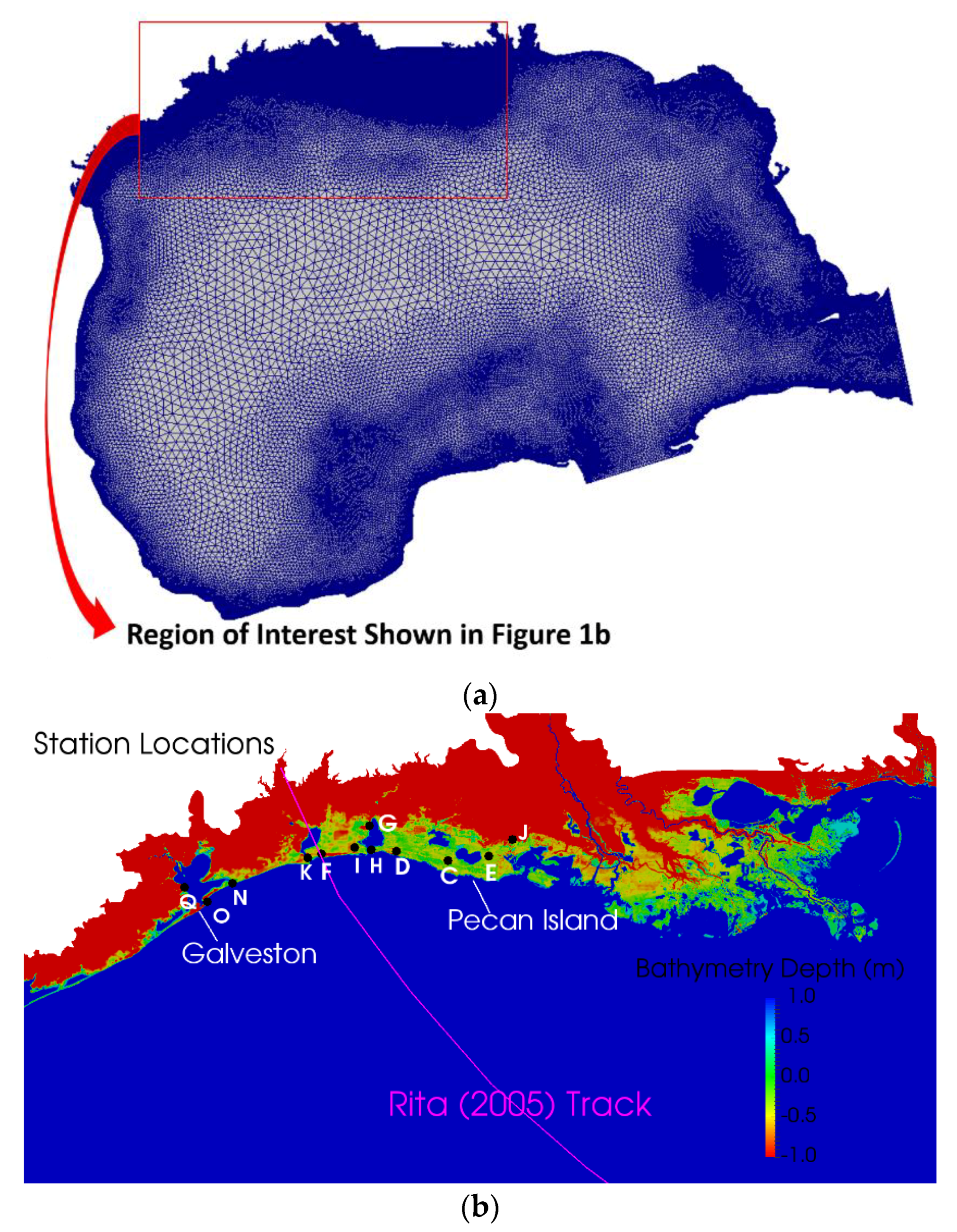
Figure 1.
Unstructured ULtralite-Levee-Removed (ULLR) [
56] mesh (
a) resolution; (
b) observation station locations with respect to Hurricane Rita track. Note that the bathymetry is artificially constrained to be between 1 m and −1 m to delineate the shoreline. Here a negative bathymetry represents above sea level.
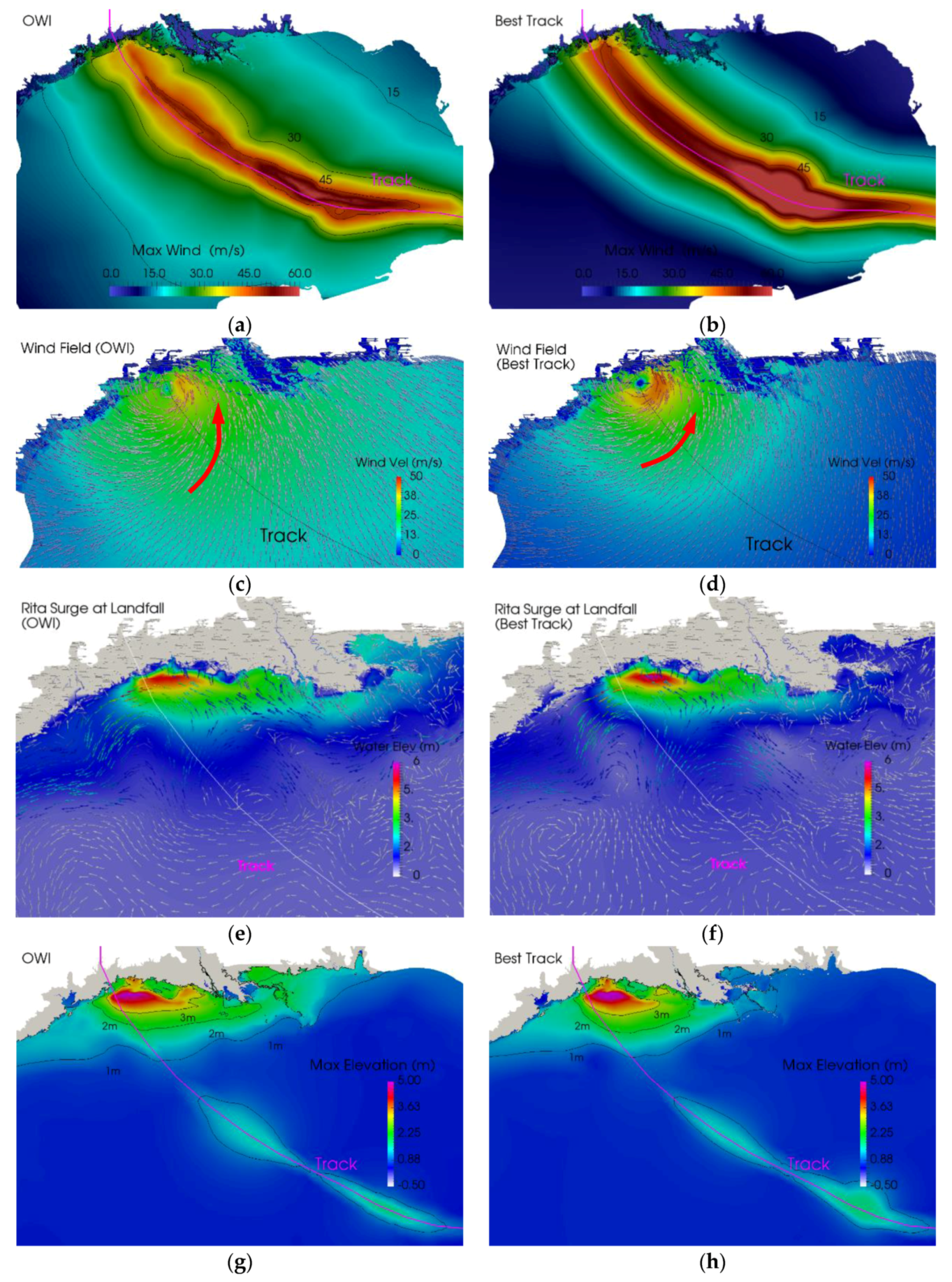
Figure 2.
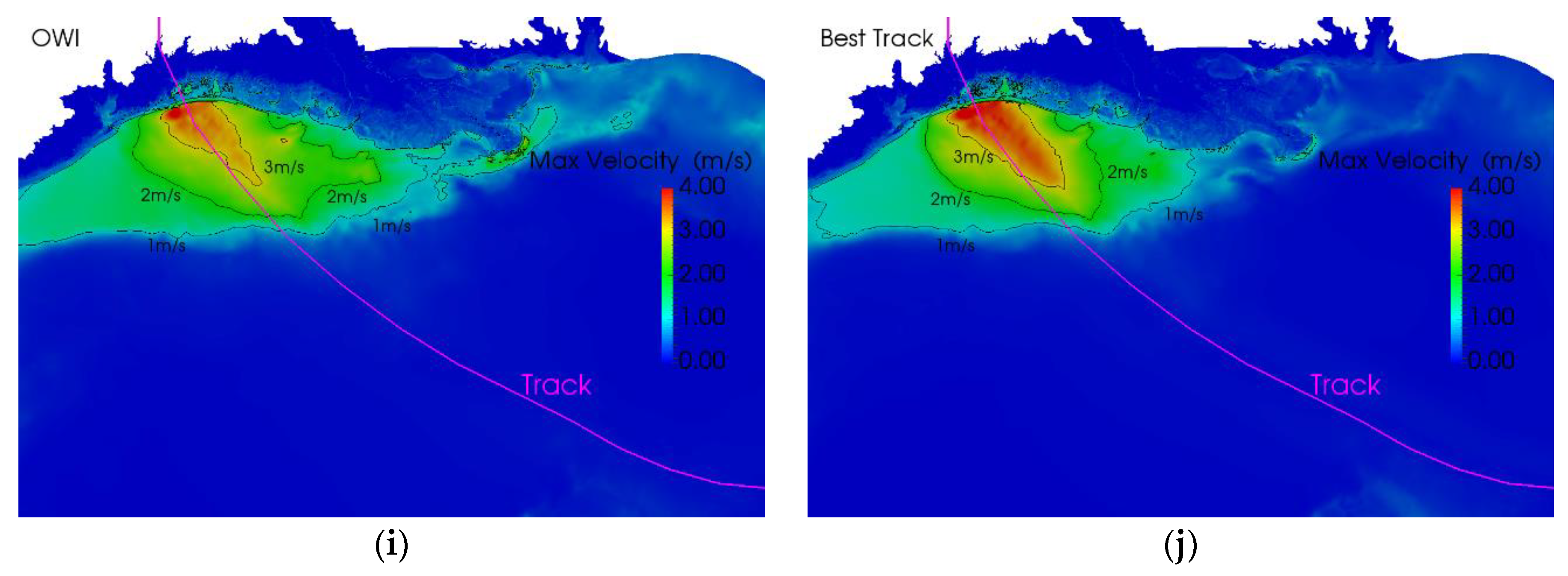
Wind field and storm surge hindcast results using Oceanweather Inc. (OWI) (a,c,e,g,i) and Best track in Generalized Asymmetric Holland Model (GAHM) − NWS = 20 option (b,d,f,h,j), (a,b) maximum wind track; (c,d) Wind vector at 8:30 a.m., 24 September of 2005; (e,f) Water elevation and velocity vector at 8:30 a.m., 24 September of 2005; (g,h) maximum water elevation; (i,j) maximum water velocity.
Figure 2.
Wind field and storm surge hindcast results using Oceanweather Inc. (OWI) (a,c,e,g,i) and Best track in Generalized Asymmetric Holland Model (GAHM) − NWS = 20 option (b,d,f,h,j), (a,b) maximum wind track; (c,d) Wind vector at 8:30 a.m., 24 September of 2005; (e,f) Water elevation and velocity vector at 8:30 a.m., 24 September of 2005; (g,h) maximum water elevation; (i,j) maximum water velocity.
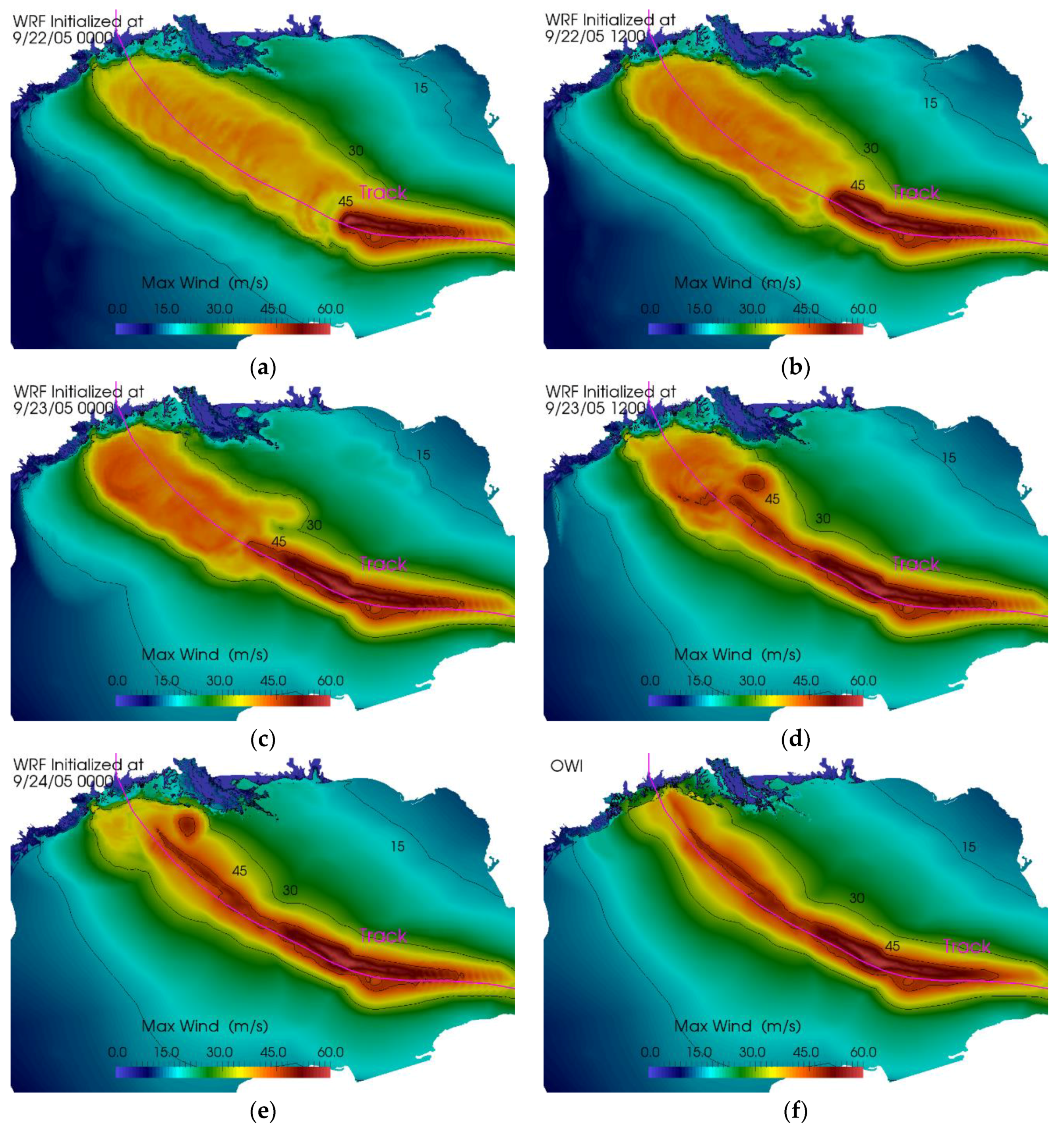
Figure 3.
Rita maximum wind track plots using wind fields from WRF and OWI models. (a) WRF Run 1, (b) WRF Run 2, (c) WRF Run 3, (d) WRF Run 4, (e) WRF Run 5, and (f) OWI.
Figure 3.
Rita maximum wind track plots using wind fields from WRF and OWI models. (a) WRF Run 1, (b) WRF Run 2, (c) WRF Run 3, (d) WRF Run 4, (e) WRF Run 5, and (f) OWI.
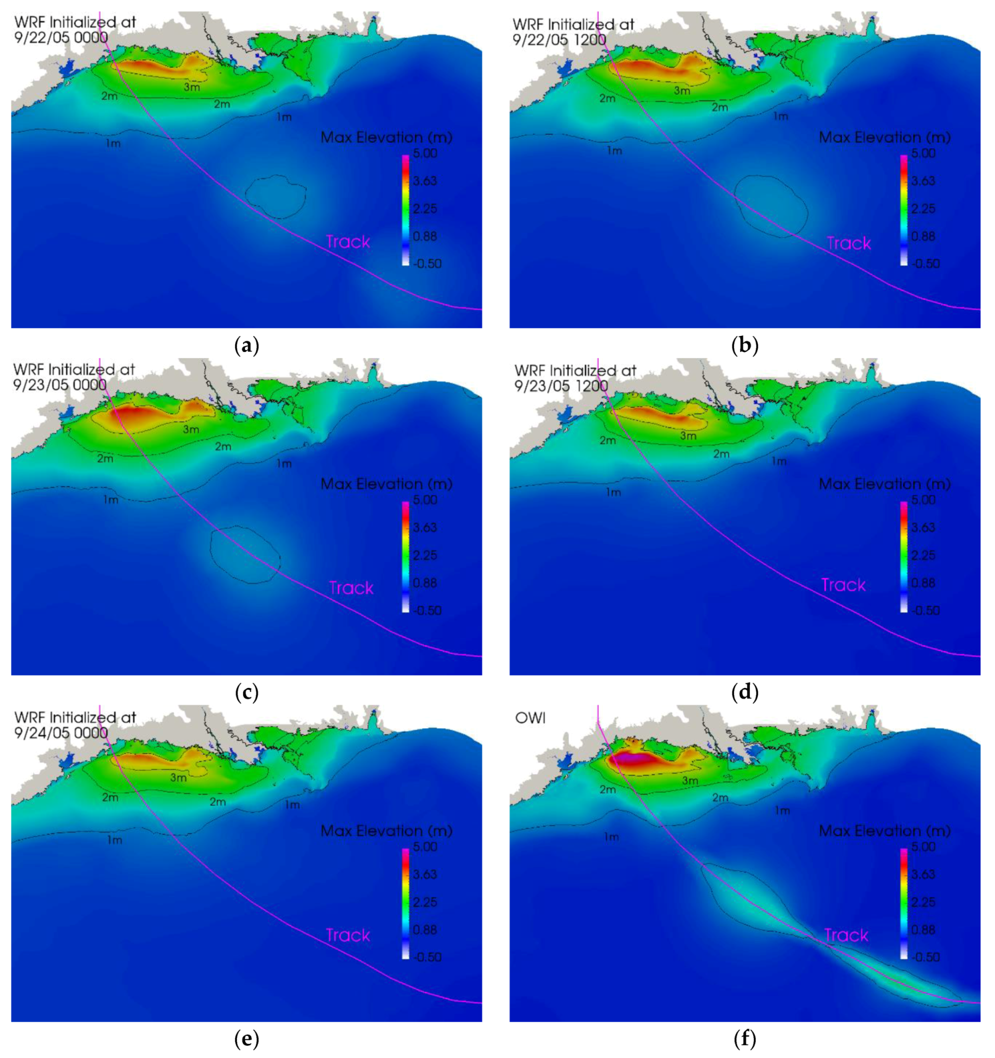
Figure 4.
Rita maximum water elevation from ADvanced CIRCulation + Simulating Waves Nearshore (ADCIRC+SWAN) simulation results using wind fields from WRF and OWI models. (a) WRF Run 1, (b) WRF Run 2, (c) WRF Run 3, (d) WRF Run 4, (e) WRF Run 5, and (f) OWI.
Figure 4.
Rita maximum water elevation from ADvanced CIRCulation + Simulating Waves Nearshore (ADCIRC+SWAN) simulation results using wind fields from WRF and OWI models. (a) WRF Run 1, (b) WRF Run 2, (c) WRF Run 3, (d) WRF Run 4, (e) WRF Run 5, and (f) OWI.
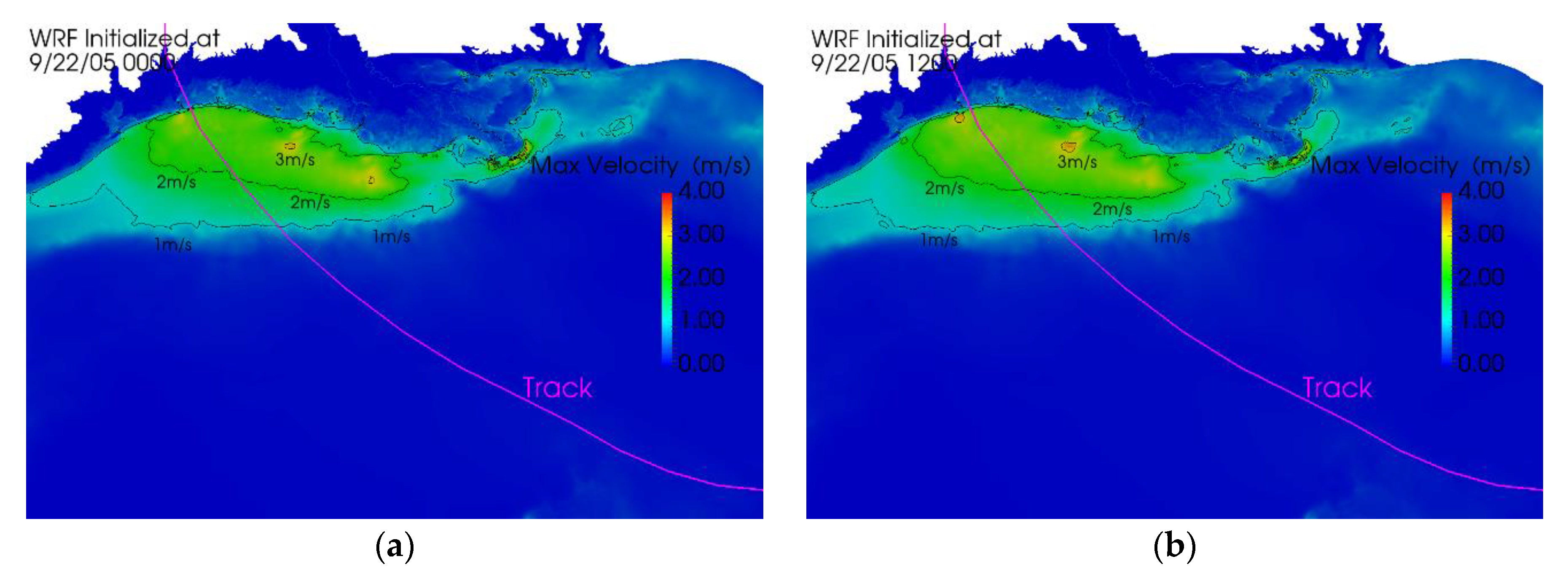
Figure 5.
Rita maximum water velocity from ADCIRC+SWAN simulation results using wind fields from WRF and OWI models. (a) WRF Run 1, (b) WRF Run 2, (c) WRF Run 3, (d) WRF Run 4, (e) WRF Run 5, and (f) OWI.
Figure 5.
Rita maximum water velocity from ADCIRC+SWAN simulation results using wind fields from WRF and OWI models. (a) WRF Run 1, (b) WRF Run 2, (c) WRF Run 3, (d) WRF Run 4, (e) WRF Run 5, and (f) OWI.
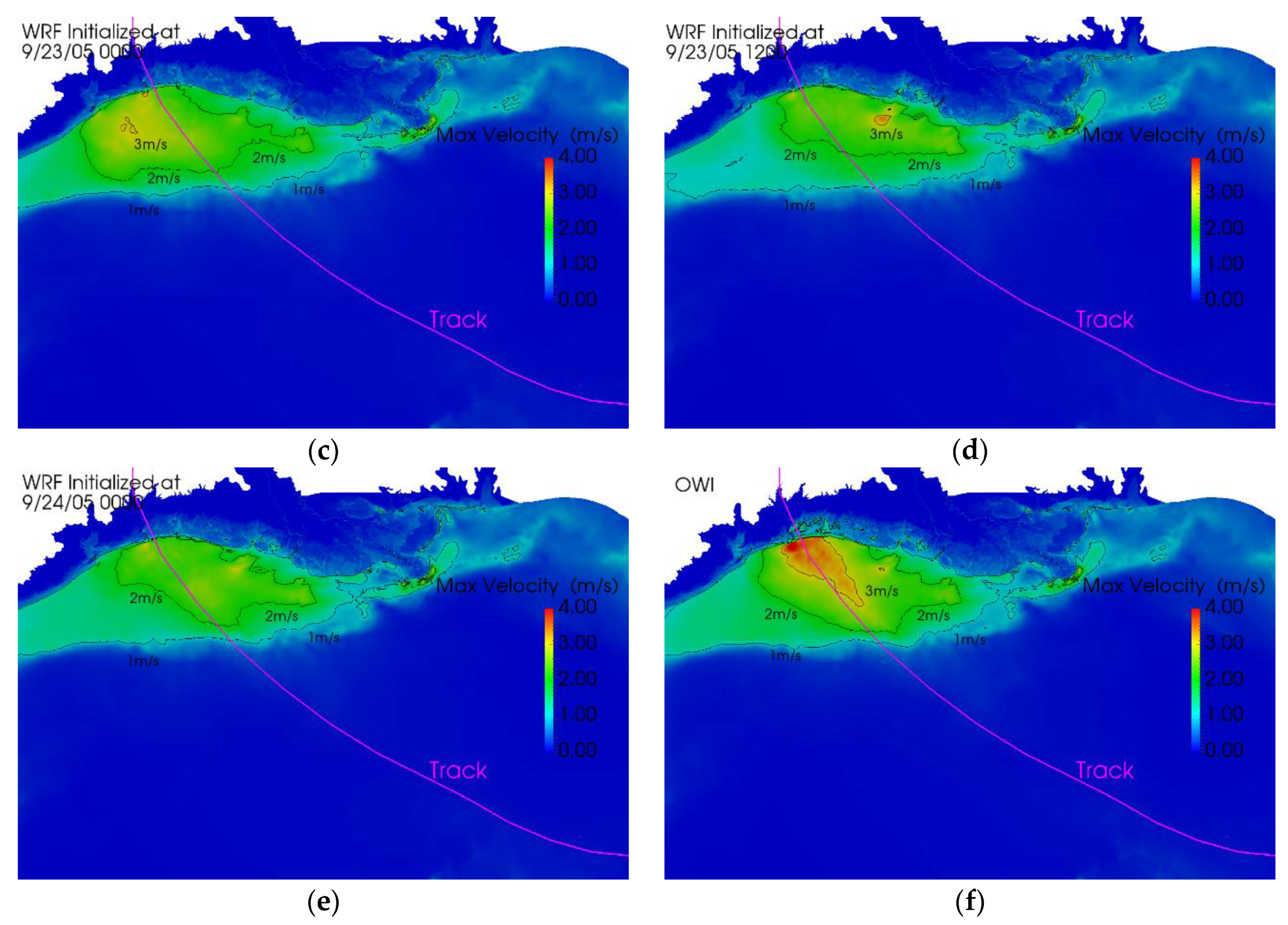
Figure 6.
Differences and contrasts between OWI hindcast and WRF Run 3—initialized at 9/23/05 0000 forecast results of Hurricane Rita storm surges: (
a) difference of maximum wind speed, (
b) contrast of wind vectors at landfall, (
c) difference of maximum water elevation, and (
d) difference of water velocity. The black dots are the locations of eight stations listed in
Table 2.
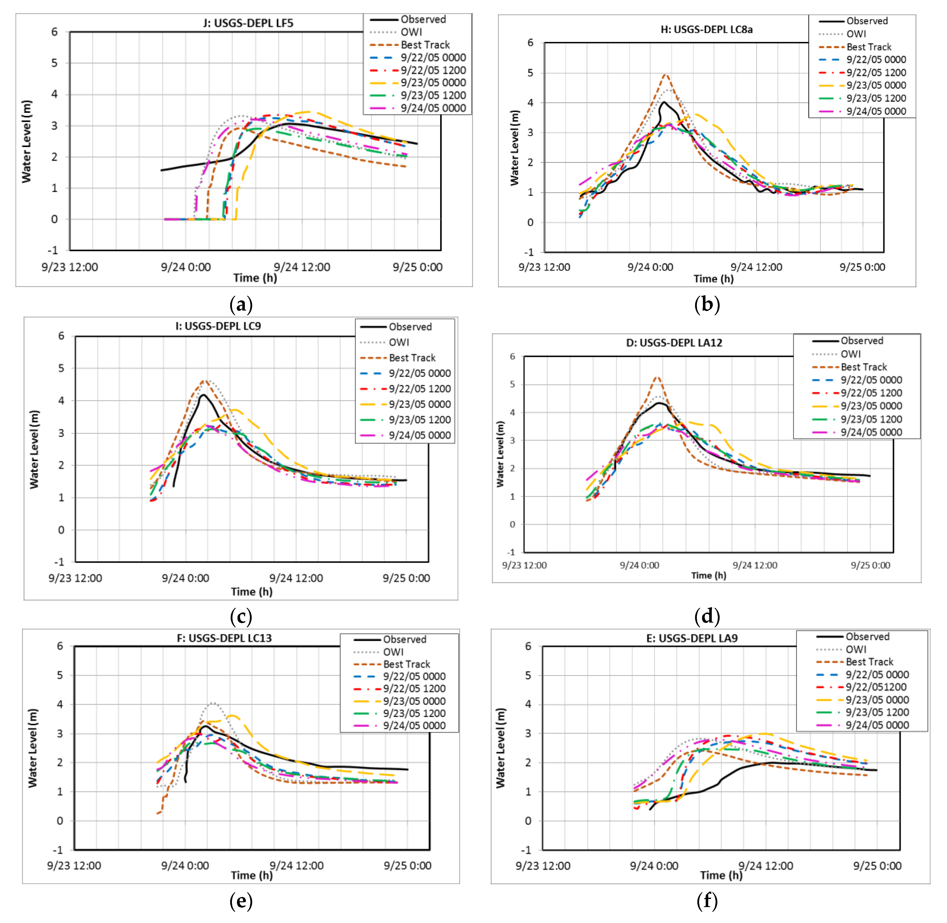
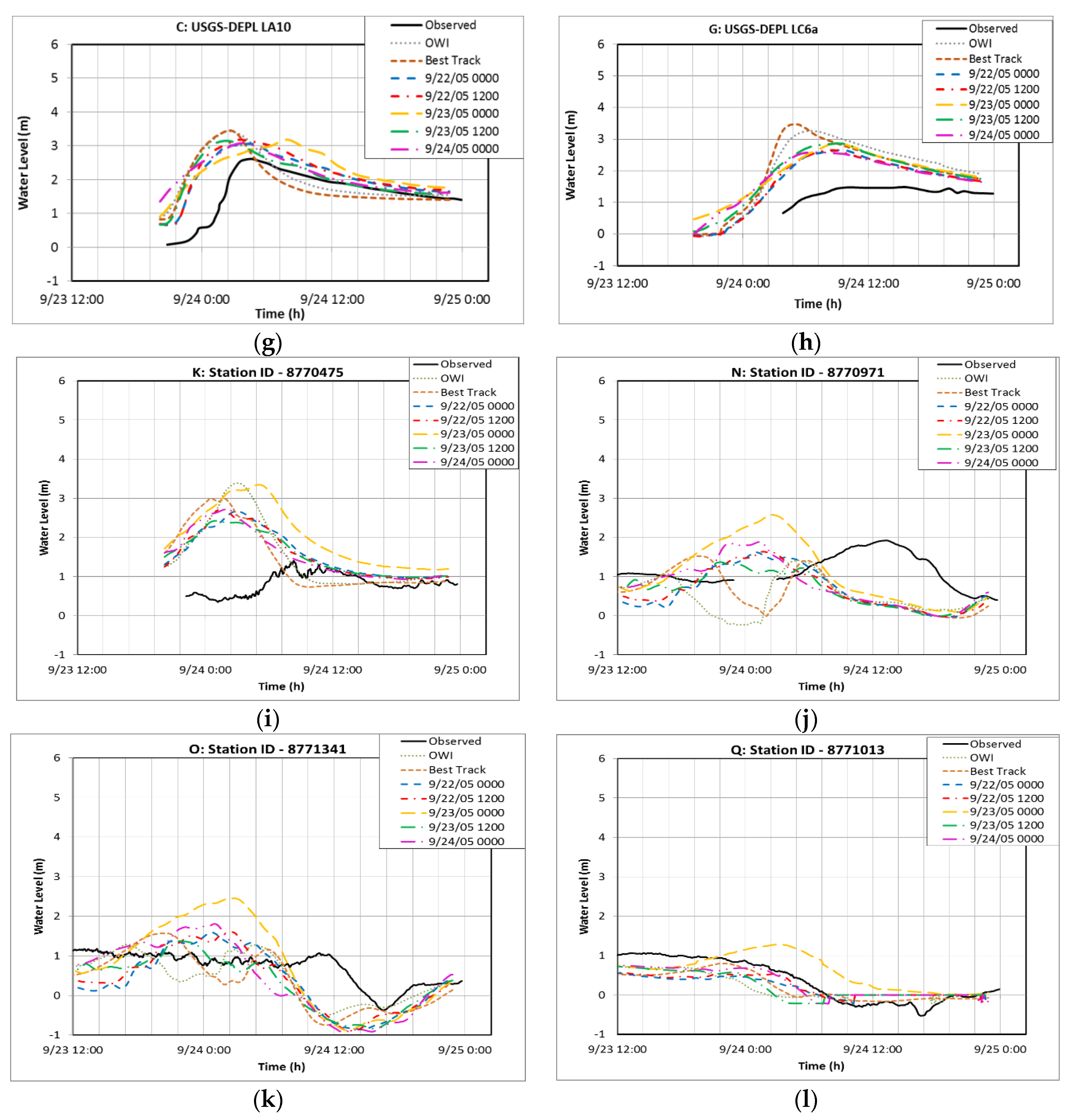
Figure 7.
Effect of wind fields from WRF, OWI, and Best track in GAHM models: Observed and ADCIRC+SWAN modeled significant water level time series at different observation stations during the time of Hurricane Rita (9/22-25/05). (a) J—USGS-DEPL LF5; (b) H—USGS-DEPL LC8a; (c) I—USGS-DEPL LC9; (d) D—USGS-DEPL LA12; (e) F—USGS-DEPL LC13; (f) E—USGS-DEPL LA9; (g) C—USGS-DEPL LA10; (h) G—USGS-DEPL LC6a; (i) K—ID 8770570, Sabine Pass North, TX; (j) N—ID 8770971, Rollover Pass, TX; (k) O—ID 8771341, Galveston Bay Entrance, North Jetty, TX; (l) Q—ID 8771013, Eagle Point, Galveston Bay, TX.
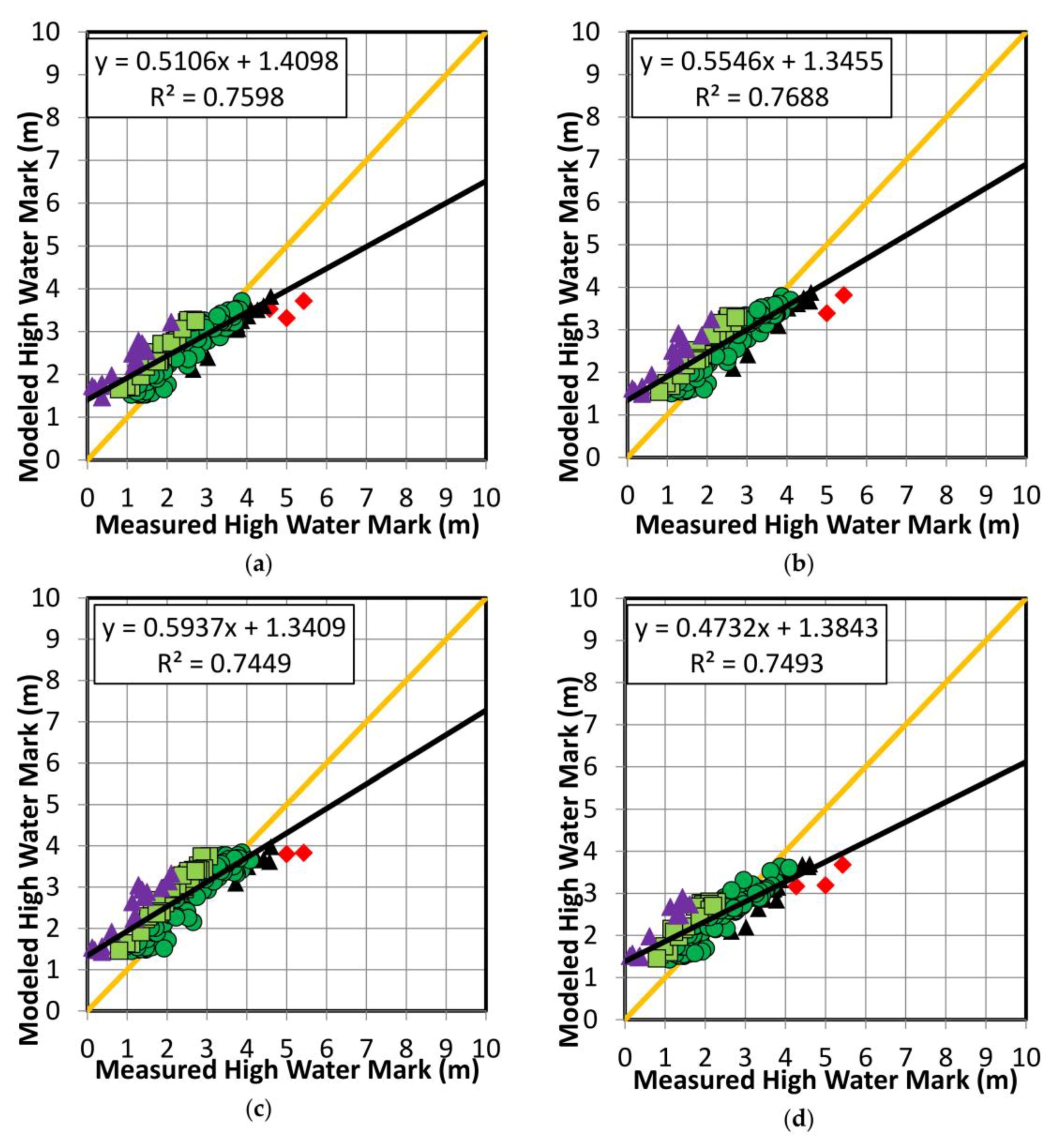
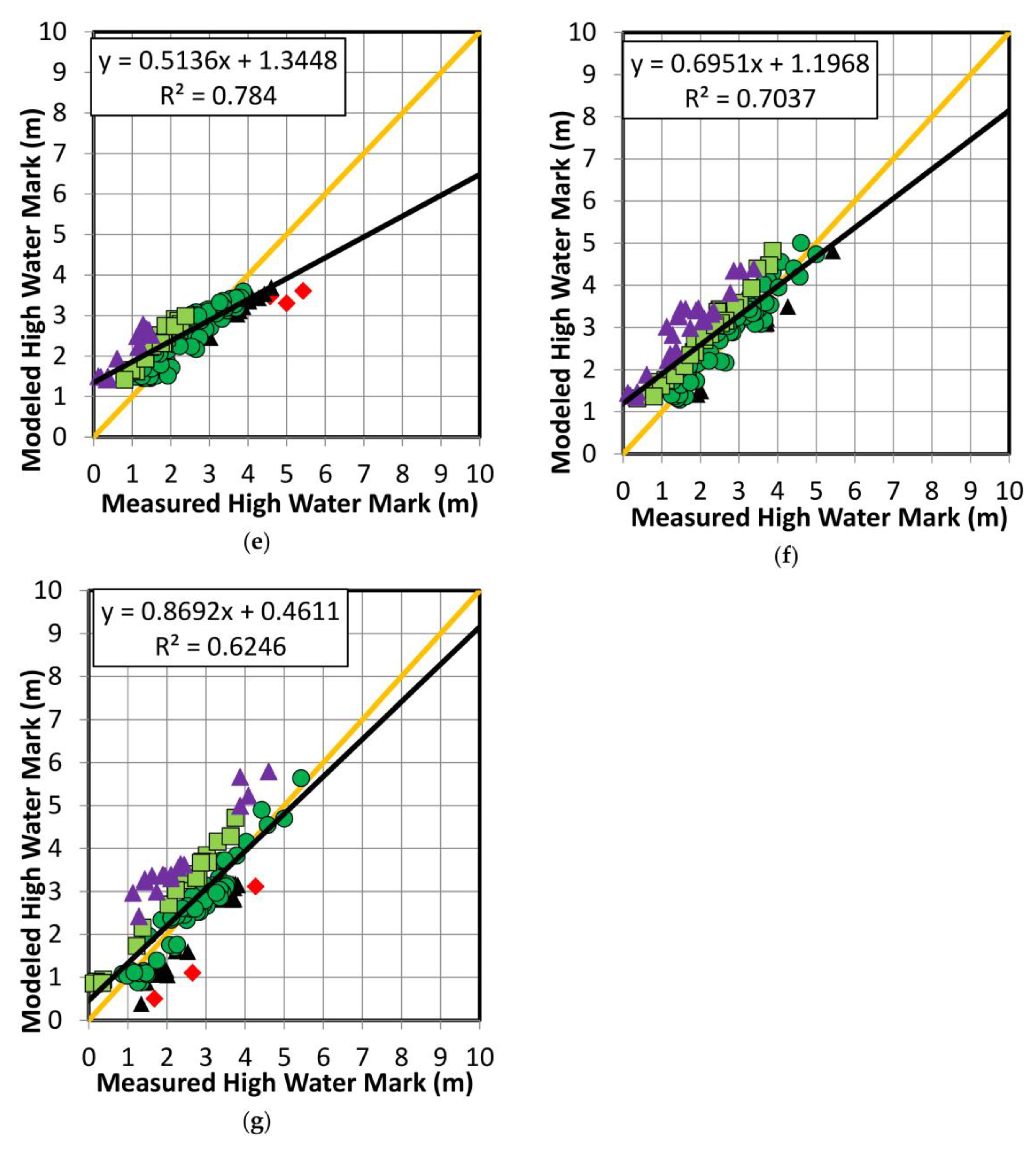
Figure 8.
Scatter plots of Rita high water marks (HWM’s) from ADCIRC+SWAN simulations using wind fields from WRF, OWI, and Best track in GAHM models. (a) WRF Run 1, (b) WRF Run 2, (c) WRF Run 3, (d) WRF Run 4, (e) WRF Run 50, (f) OWI, and (g) Best track in GAHM. Red diamond and black triangles indicate underprediction by the model; purple triangles and light green squares indicate overprediction. Dark green circles indicate a match within 0.5 m. The black line represents the best fit lines. The orange line is the parity.
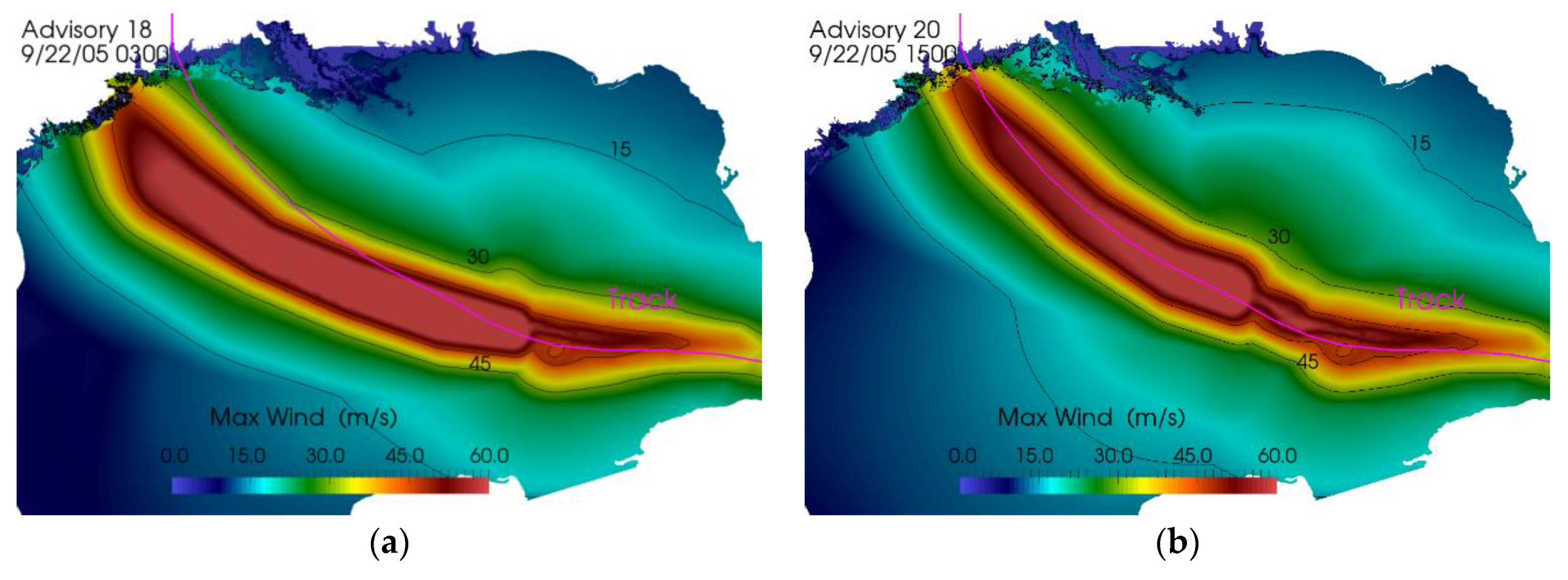
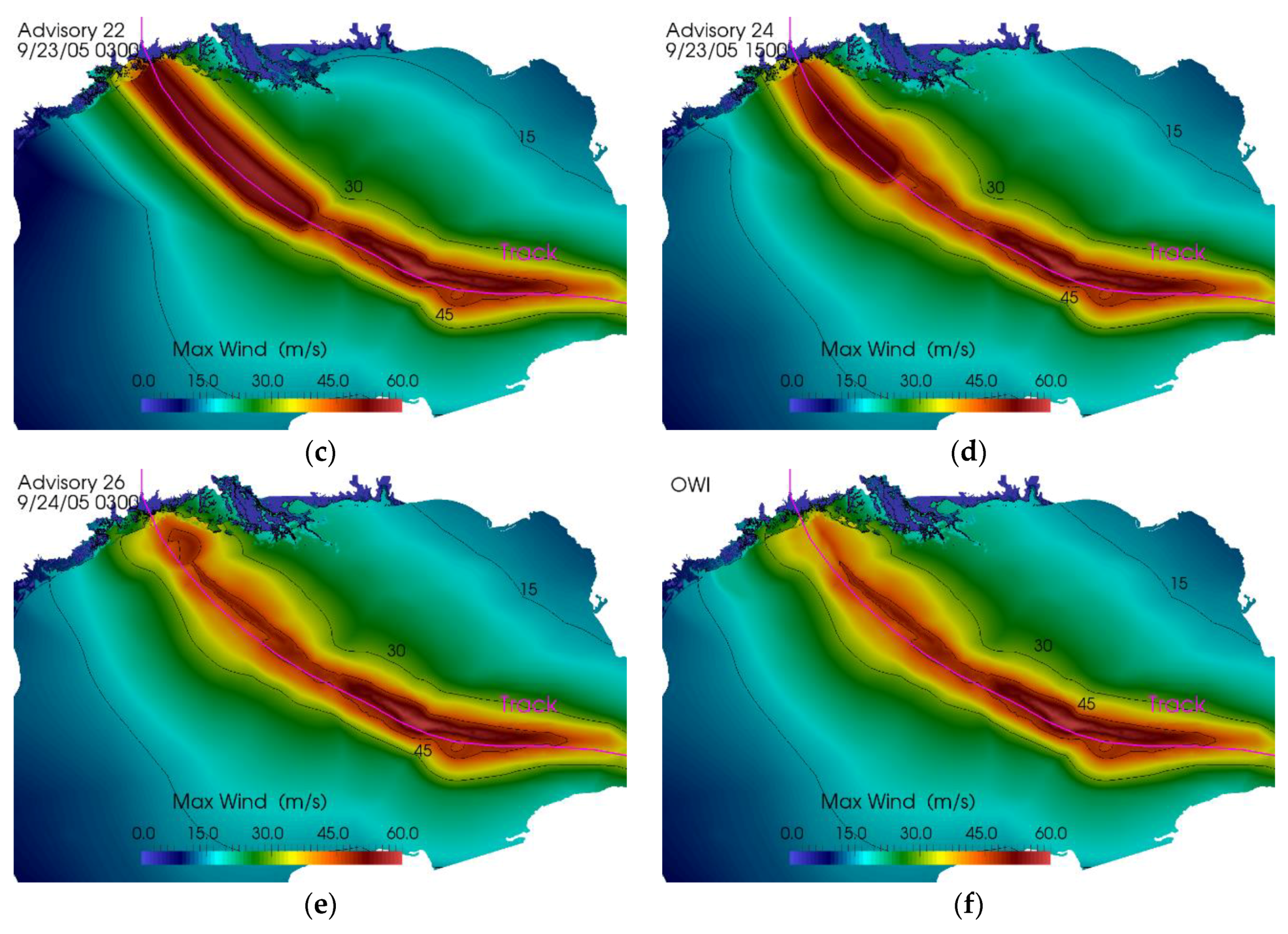
Figure 9.
Rita maximum wind track plots using wind fields from Advisories in GAHM and OWI models. (a) Advisory 18—Adv Run 1, (b) Advisory 20—Adv Run 2, (c) Advisory 22—Adv Run 3, (d) Advisory 24—Adv Run 4, (e) Advisory 26—Adv Run 5, and (f) OWI.
Figure 9.
Rita maximum wind track plots using wind fields from Advisories in GAHM and OWI models. (a) Advisory 18—Adv Run 1, (b) Advisory 20—Adv Run 2, (c) Advisory 22—Adv Run 3, (d) Advisory 24—Adv Run 4, (e) Advisory 26—Adv Run 5, and (f) OWI.
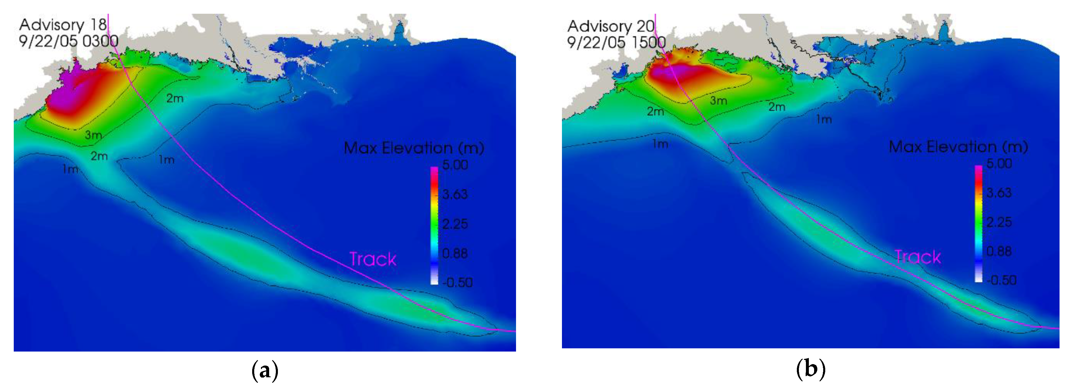
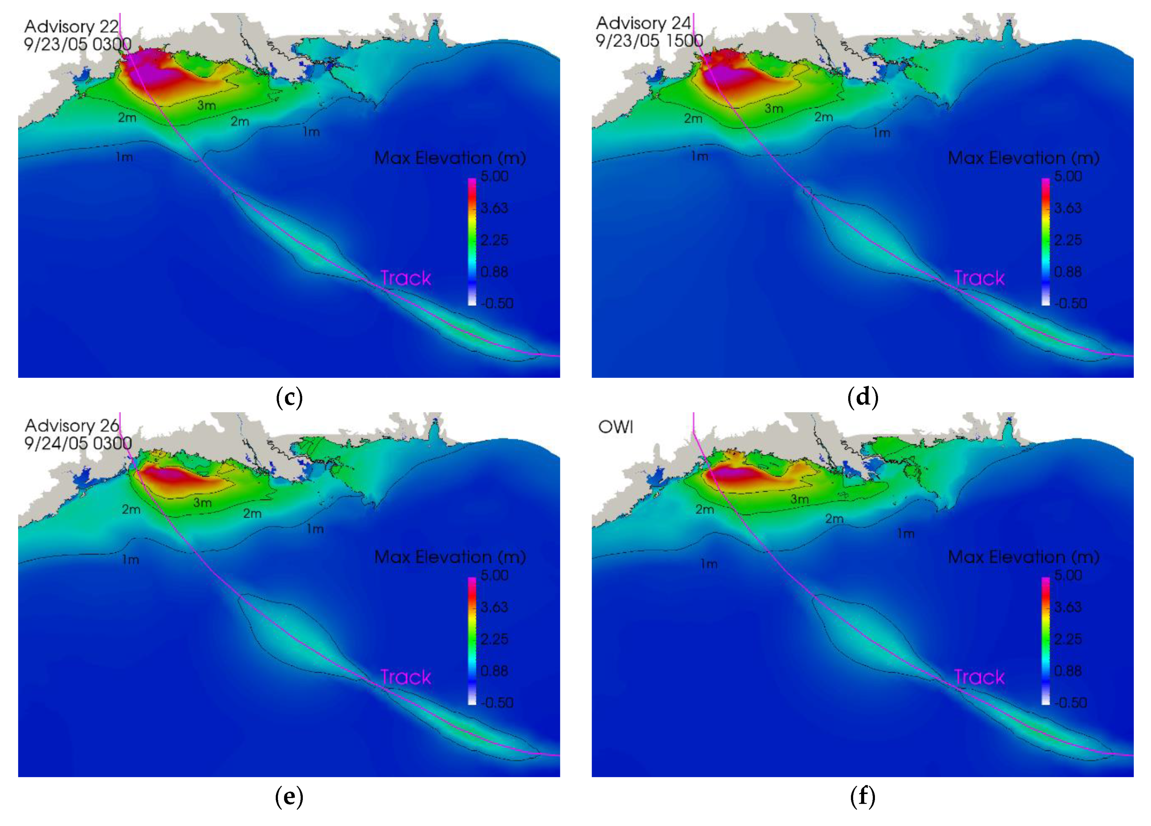
Figure 10.
Rita maximum water elevation from ADCIRC+SWAN simulation results using wind fields from advisories in GAHM and OWI models. (a) Advisory 18—Adv Run 1, (b) Advisory 20—Adv Run 2, (c) Advisory 22—Adv Run 3, (d) Advisory 24—Adv Run 4, (e) Advisory 26—Adv Run 5, and (f) OWI.
Figure 10.
Rita maximum water elevation from ADCIRC+SWAN simulation results using wind fields from advisories in GAHM and OWI models. (a) Advisory 18—Adv Run 1, (b) Advisory 20—Adv Run 2, (c) Advisory 22—Adv Run 3, (d) Advisory 24—Adv Run 4, (e) Advisory 26—Adv Run 5, and (f) OWI.
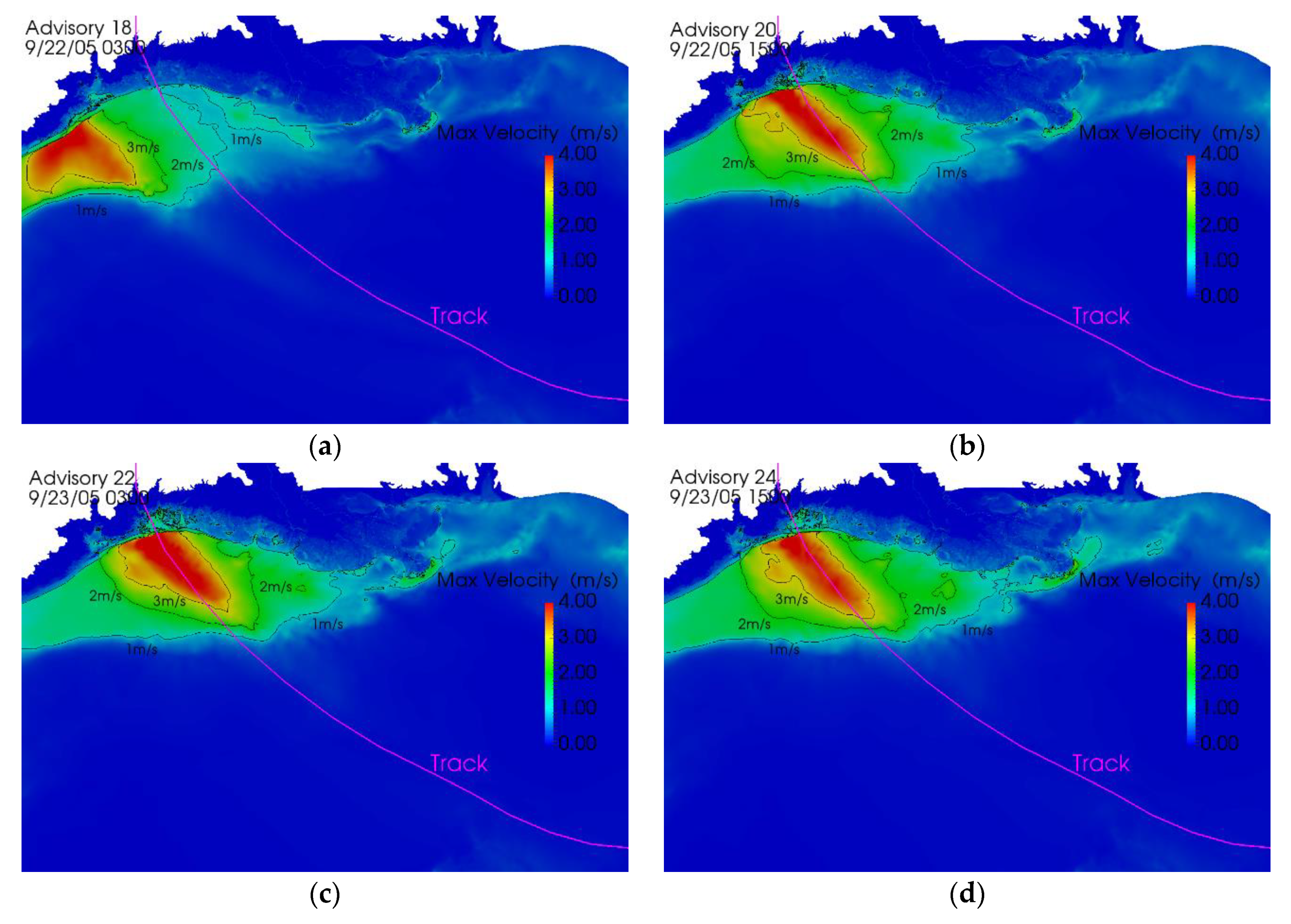
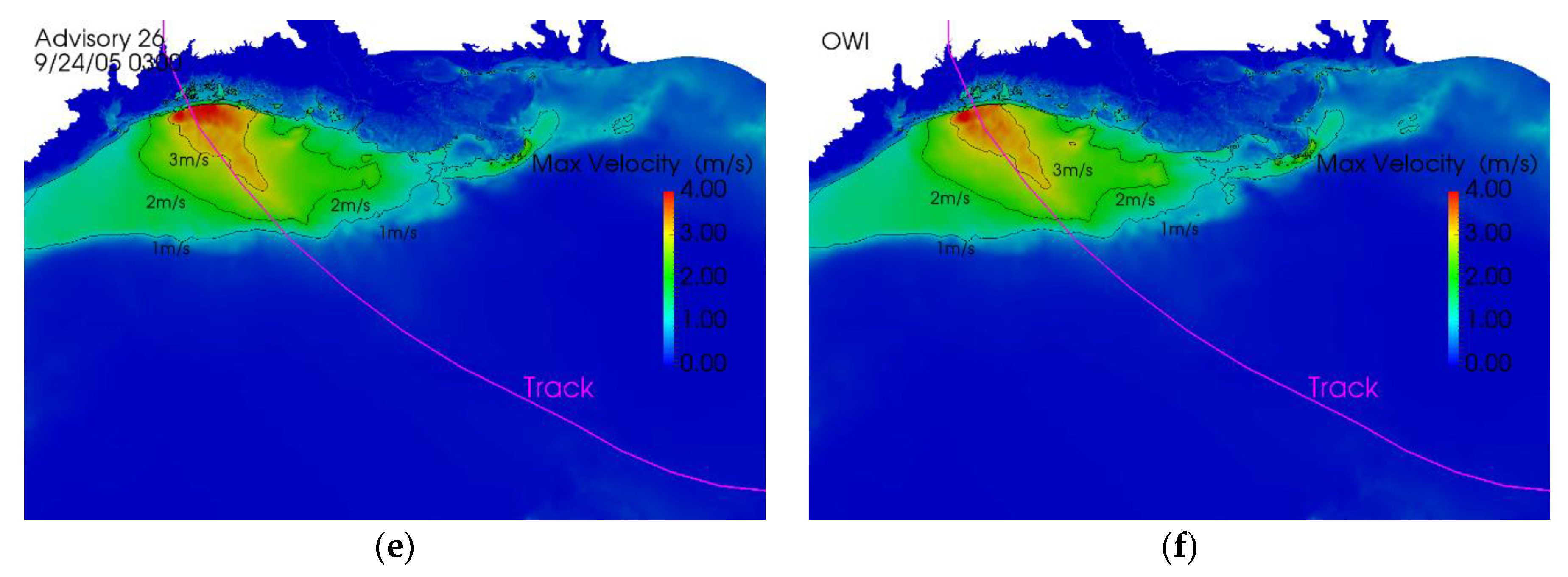
Figure 11.
Rita maximum water velocity from ADCIRC+SWAN simulation results using wind fields from advisories in GAHM and OWI models. (a) Advisory 18—Adv Run 1, (b) Advisory 20—Adv Run 2, (c) Advisory 22—Adv Run 3, (d) Advisory 24—Adv Run 4, (e) Advisory 26—Adv Run 5, and (f) OWI.
Figure 11.
Rita maximum water velocity from ADCIRC+SWAN simulation results using wind fields from advisories in GAHM and OWI models. (a) Advisory 18—Adv Run 1, (b) Advisory 20—Adv Run 2, (c) Advisory 22—Adv Run 3, (d) Advisory 24—Adv Run 4, (e) Advisory 26—Adv Run 5, and (f) OWI.
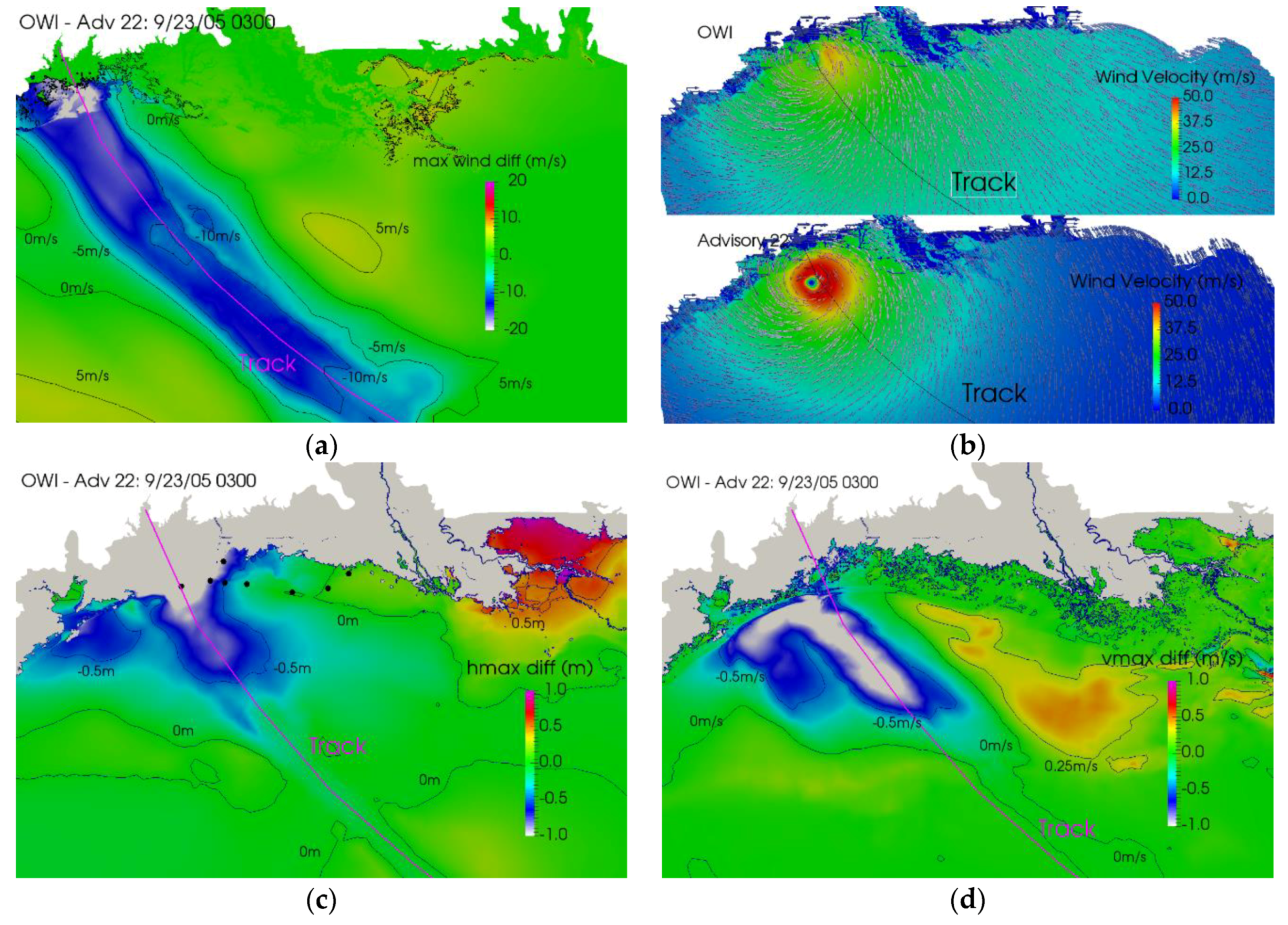
Figure 12.
Differences and contrasts between OWI and Adv Run 3 hindcast results of Hurricane Rita storm surges: (
a) difference of maximum wind speed, (
b) contrast of wind vectors at landfall, (
c) difference of maximum water elevation, and (
d) difference of water velocity. The black dots are the locations of eight stations listed in
Table 2.
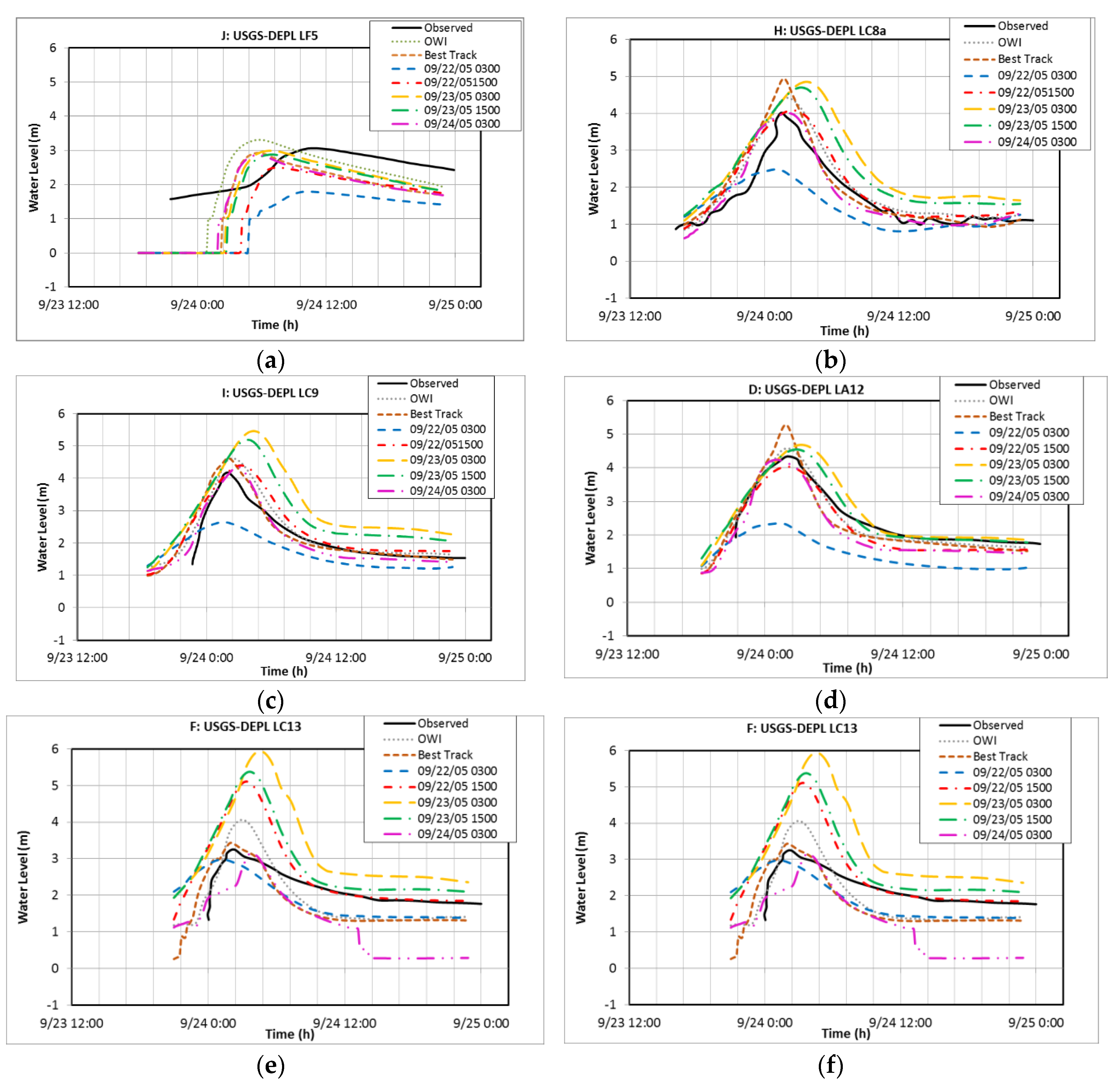
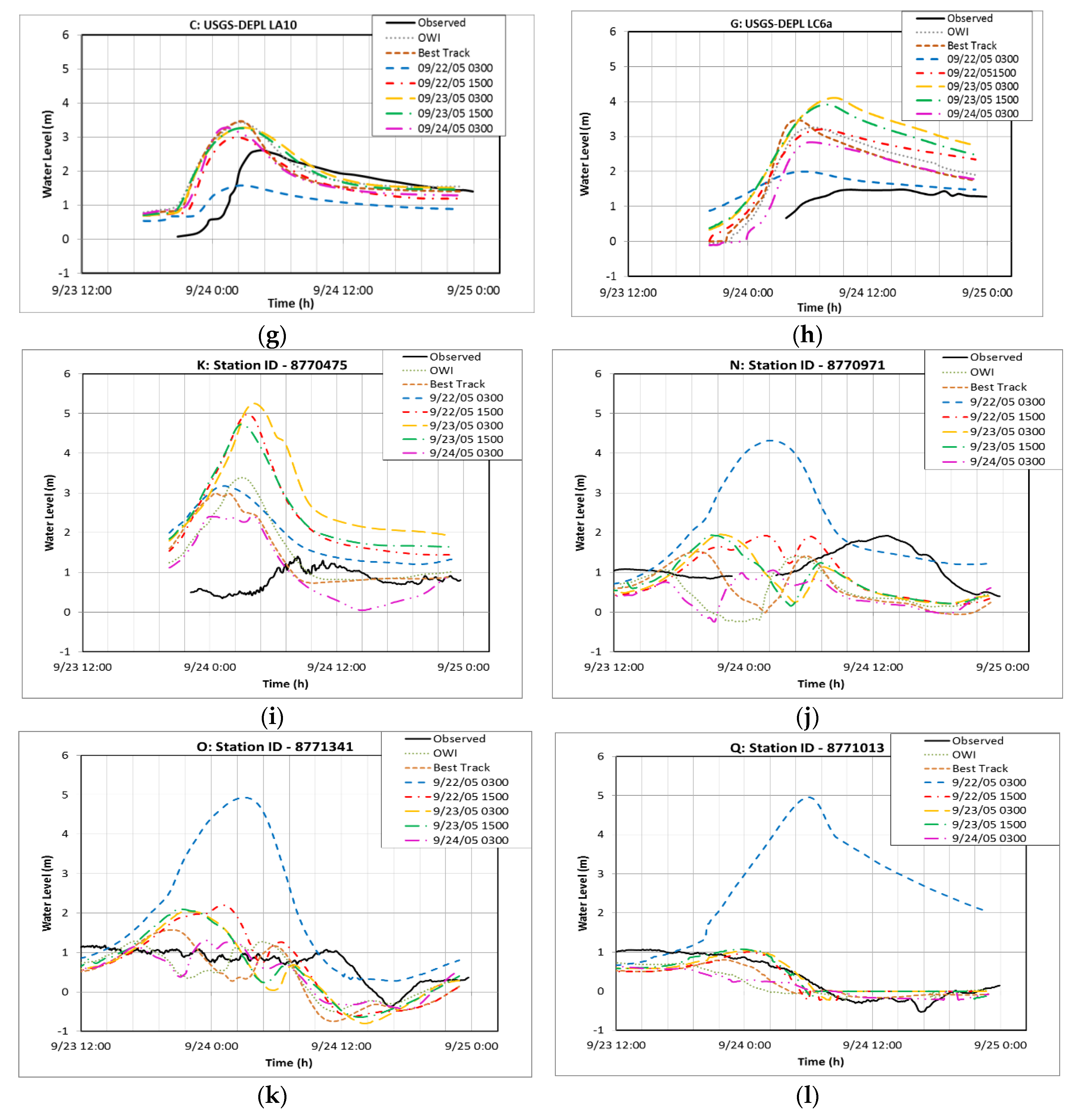
Figure 13.
Effect of wind fields from Advisories in GAHM and OWI models: Observed and ADCIRC+SWAN modeled significant water level time series at different observation stations during the time of Hurricane Rita (9/22-25/05). (a) J—USGS-DEPL LF5; (b) H—USGS-DEPL LC8a; (c) I—USGS-DEPL LC9; (d) D—USGS-DEPL LA12; (e) F—USGS-DEPL LC13; (f) E—USGS-DEPL LA9; (g) C—USGS-DEPL LA10; (h) G—USGS-DEPL LC6a; (i) K—ID 8770570, Sabine Pass North, TX; (j) N—ID 8770971, Rollover Pass, TX; (k) O—ID 8771341, Galveston Bay Entrance, North Jetty, TX; (l) Q—ID 8771013, Eagle Point, Galveston Bay, TX. (Advisory 18—Adv Run 1: 9/22/05 0300; Advisory 20—Adv Run 2: 9/22/05 1500; Advisory 22—Adv Run 3: 9/23/05 0300; Advisory 24—Adv Run 4: 9/23/05 1500; Advisory 26—Adv Run 5: 9/24/05 0300).
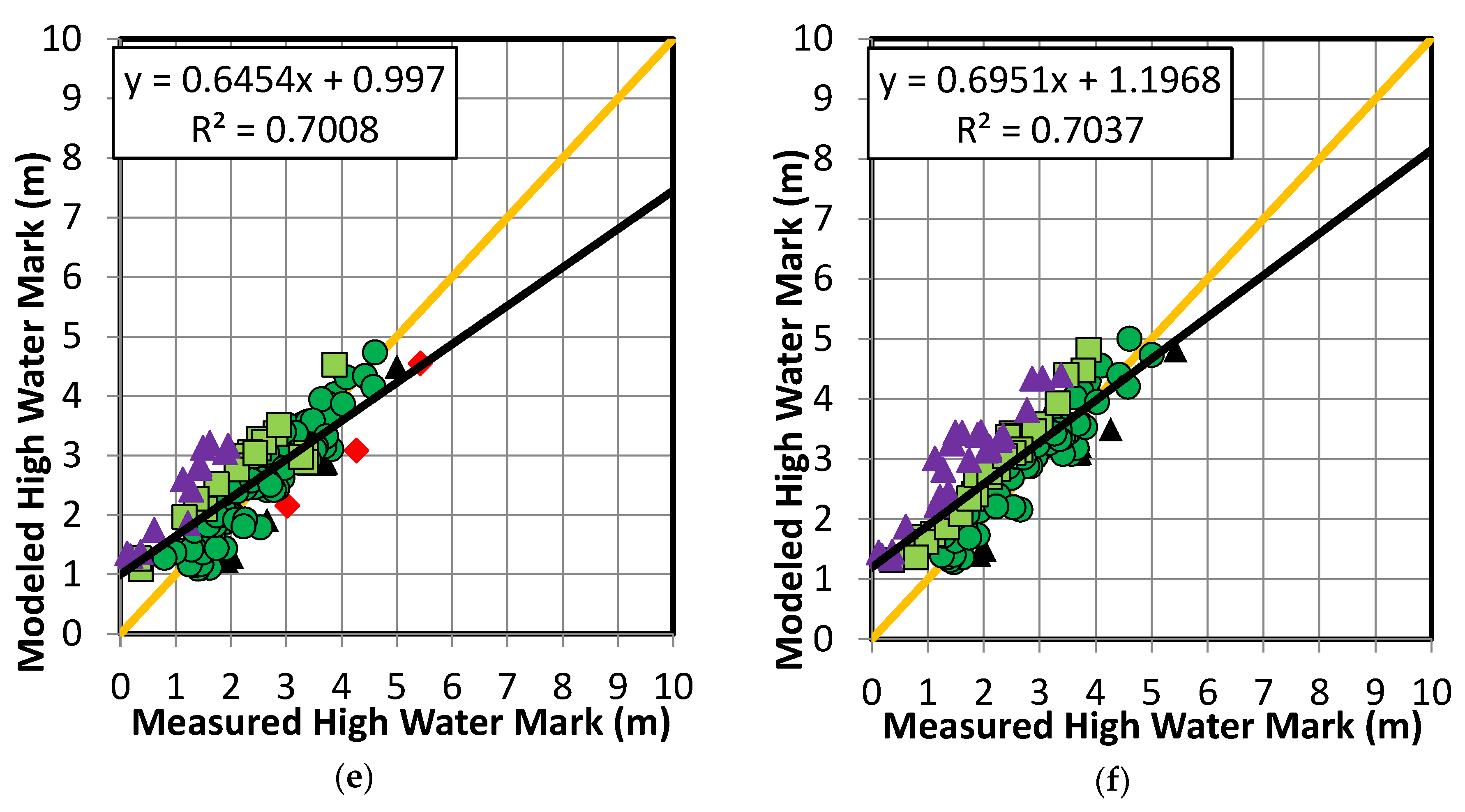
Figure 14.
Scatter plots of Rita HWM’s from ADCIRC+SWAN simulations using wind fields from advisories in GAHM and OWI. (a) Advisory 18—Adv Run 1, (b) Advisory 20—Adv Run 2, (c) Advisory 22—Adv Run 3, (d) Advisory 24—Adv Run 4, (e) Advisory 26—Adv Run 5, and (f) OWI. Red diamond and black triangles indicate underprediction by the model; purple triangles and light green squares indicate overprediction. Dark green circles indicate a match within 0.5 m. The black line represents the best fit lines. The orange line represents the parity.
Table 1.
Weather Research and Forecasting (WRF) model configuration.
Table 1.
Weather Research and Forecasting (WRF) model configuration.
| Parameter | Configuration |
|---|
| Initial conditions | NCEP 1° by 1° final analysis (FNL) |
| Map projection | Lambert |
| Horizontal grid distance | 15 km |
| NCEP time interval | 6 h |
| Time step | 60 |
| Microphysics | WSM6 |
| Longwave radiation | RRTM |
| Shortwave radiation | Dudhia |
| Cumulus parameterization | Kain-Fritsch |
| PBL parameterization | Yonsei University (YSU) scheme |
| Land Surface option | NOAH land surface model |
Table 2.
Locations of United States Geological Survey (USGS) [
64] Deployed (DEPL) observation stations. Note: LA10, LC13, LF5, etc. are identification tags for station locations.
Table 2.
Locations of United States Geological Survey (USGS) [
64] Deployed (DEPL) observation stations. Note: LA10, LC13, LF5, etc. are identification tags for station locations.
| ID | Station | Longitude (°) | Latitude (°) |
|---|
| C | USGS-DEPL LA10 | −92.67552 | 29.70658 |
| D | USGS-DEPL LA12 | −93.11494 | 29.7861 |
| E | USGS-DEPL LA9 | −92.32792 | 29.74476 |
| F | USGS-DEPL LC13 | −93.75285 | 29.76407 |
| G | USGS-DEPL LC6a | −93.34333 | 30.00432 |
| H | USGS-DEPL LC8a | −93.32886 | 29.79764 |
| I | USGS-DEPL LC9 | −93.47052 | 29.81823 |
| J | USGS-DEPL LF5 | −92.12703 | 29.88604 |
| 8770570 | Sabine Pass North, TX | −93.87000 | 29.72833 |
| 8770971 | Rollover Pass, TX | −94.51000 | 29.51500 |
| 8771341 | Galveston Bay Entrance, North Jetty, TX | −94.72500 | 29.35667 |
| 8771013 | Eagle Point, Galveston Bay, TX | −94.91833 | 29.48000 |
Table 3.
Description of WRF runs and initialization times for surge forecasts.
Table 3.
Description of WRF runs and initialization times for surge forecasts.
| Simulation Number | Initialization Time (UTC) | Hours before Landfall |
|---|
| WRF Run 1 | 9/22/2005 0000 | 56 |
| WRF Run 2 | 9/22/2005 1200 | 44 |
| WRF Run 3 | 9/23/2005 0000 | 32 |
| WRF Run 4 | 9/23/2005 1200 | 20 |
| WRF Run 5 | 9/24/2005 0000 | 8 |
Table 4.
HWM error statistics for Rita surge forecast and hindcast using wind fields from WRF, OWI, and Best Track in GAHM.
Table 4.
HWM error statistics for Rita surge forecast and hindcast using wind fields from WRF, OWI, and Best Track in GAHM.
| Case | | ERMS (m) | (m) | BMN (-) | σ (m) | SI (-) | MAE (m) | ENORM (-) | Dry | Wet |
|---|
| WRF Run 1 | 0.760 | 0.459 | 0.256 | 0.108 | 0.629 | 0.407 | 0.534 | 0.068 | 10 | 134 |
| WRF Run 2 | 0.769 | 0.443 | 0.295 | 0.125 | 0.598 | 0.387 | 0.520 | 0.068 | 10 | 134 |
| WRF Run 3 | 0.745 | 0.515 | 0.391 | 0.166 | 0.604 | 0.392 | 0.564 | 0.077 | 9 | 135 |
| WRF Run 4 | 0.749 | 0.470 | 0.153 | 0.065 | 0.671 | 0.435 | 0.525 | 0.070 | 9 | 135 |
| WRF Run 5 | 0.784 | 0.435 | 0.208 | 0.088 | 0.628 | 0.408 | 0.511 | 0.065 | 9 | 135 |
| OWI | 0.704 | 0.598 | 0.480 | 0.203 | 0.609 | 0.394 | 0.616 | 0.088 | 7 | 137 |
| Best Track in GAHM | 0.625 | 0.591 | 0.138 | 0.056 | 0.759 | 0.480 | 0.625 | 0.081 | 23 | 121 |
Table 5.
Description of Rita advisory runs and initialization times for surge forecasts.
Table 5.
Description of Rita advisory runs and initialization times for surge forecasts.
| Simulation Number | Advisory Identification | Initialization Time (UTC) | Hours before Landfall |
|---|
| Adv Run 1 | Advisory 18 | 9/22/2005 0300 | 53 |
| Adv Run 2 | Advisory 20 | 9/22/2005 1500 | 41 |
| Adv Run 3 | Advisory 22 | 9/23/2005 0300 | 29 |
| Adv Run 4 | Advisory 24 | 9/23/2005 1500 | 17 |
| Adv Run 5 | Advisory 26 | 9/24/2005 0300 | 5 |
Table 6.
HWM error statistics for Rita simulations using forecasted wind fields from archived Advisories.
Table 6.
HWM error statistics for Rita simulations using forecasted wind fields from archived Advisories.
| Case | | ERMS (m) | (m) | BMN (-) | σ (m) | SI (-) | MAE (m) | ENORM (-) | Dry | Wet |
|---|
| Advisory 18: Adv Run 1 | 0.438 | 1.050 | −0.611 | −0.253 | 0.827 | 0.529 | 0.850 | 0.151 | 48 | 96 |
| Advisory 20: Adv Run 2 | 0.568 | 0.675 | 0.091 | 0.038 | 0.820 | 0.526 | 0.659 | 0.095 | 23 | 121 |
| Advisory 22: Adv Run 3 | 0.713 | 0.496 | 0.193 | 0.080 | 0.680 | 0.436 | 0.553 | 0.069 | 36 | 108 |
| Advisory 24: Adv Run 4 | 0.615 | 0.663 | 0.266 | 0.110 | 0.773 | 0.496 | 0.620 | 0.094 | 23 | 121 |
| Advisory 26: Adv Run 5 | 0.701 | 0.423 | 0.167 | 0.071 | 0.631 | 0.409 | 0.508 | 0.062 | 9 | 135 |
| OWI (repeated) | 0.704 | 0.598 | 0.480 | 0.203 | 0.609 | 0.394 | 0.616 | 0.088 | 7 | 137 |
| Best Track (repeated) | 0.625 | 0.591 | 0.138 | 0.056 | 0.759 | 0.480 | 0.625 | 0.081 | 23 | 121 |
Table 7.
Summarized HWM error statistics for Rita surge forecast and hindcast using different wind fields.
Table 7.
Summarized HWM error statistics for Rita surge forecast and hindcast using different wind fields.
| Case | | ERMS (m) | (m) | BMN (-) | σ (m) | SI (-) | MAE (m) | ENORM (-) | Dry | Wet |
|---|
| OWI | 0.704 | 0.598 | 0.480 | 0.203 | 0.609 | 0.394 | 0.616 | 0.088 | 7 | 137 |
| Best Track in GAHM | 0.625 | 0.591 | 0.138 | 0.056 | 0.759 | 0.480 | 0.625 | 0.081 | 23 | 121 |
| WRF Run 3 | 0.745 | 0.515 | 0.391 | 0.166 | 0.604 | 0.392 | 0.564 | 0.077 | 9 | 135 |
| Adv Run 3 | 0.713 | 0.496 | 0.193 | 0.080 | 0.680 | 0.436 | 0.553 | 0.069 | 36 | 108 |


