Noise Characteristics Analysis of the Horizontal Axis Hydrokinetic Turbine Designed for Unmanned Underwater Mooring Platforms

Abstract

Operating horizontal axis hydrokinetic turbine (HAHT) generates noise affecting the ocean environment adversely. Therefore, it is essential to determine the noise characteristics of such types of HAHT, as large-scale turbine sets would release more noise pollution to the ocean. Like other rotating machinery, the hydrodynamic noise generated by the rotating turbine has been known to be the most important noise source. In the present work, the transient turbulent flow field of the HAHT is obtained by incompressible large eddy simulation, thereafter, the Ffowcs Williams and Hawkings acoustic analogy formulation is carried out to predict the noise generated from the pressure fluctuations of the blade surface. The coefficient of power is compared with the experimental results, with a good agreement being achieved. It is seen from the pressure contours that the 80% span of the blade has the most severe pressure fluctuations, which concentrate on the region of leading the edge of the airfoil and the suction surface of the airfoil. Then, the noise characteristics around a single turbine are systematically studied, in accordance with the results of the flow field. The noise characteristics around the whole turbine are also investigated to determine the directionality of the noise emission of HAHT.

1. Introduction

Unmanned underwater mooring platforms (UUMPs), which are anchored to the seabed using mooring cables, could perform various functions in the ocean with a long period of time, typically ranging from several months to several years. In the present stage, most of the battery-powered UUMPs face the problem of an insufficiency if energy supply during the service period, because of the limited battery capacity and uninterrupted energy consumption by the electronic devices. Thus, the energy problem of the UUMPs is a significant issue to be considered in the design process.

Marine renewable energy is a huge potential energy resource, including ocean thermal energy [1], ocean surface solar energy [2], ocean wave energy [3], and ocean current energy [4], which could potentially recharge the batteries of the UUMPs. As most of the UUMPs are expected to carry out fix-point missions for long durations, ocean thermal energy and ocean surface solar energy are not suitable for continuous energy supply of UUMPs. For the utilization of ocean wave energy, conversion devices are also expected to be located near the ocean surface, which is infeasible for deep-water UUMPs. As a matter of fact, UUMPs are often placed where ocean currents are consistently available [5], which could provide an effective energy supply to recharge the UUMPs. Hydrokinetic turbines are the primary energy conversion devices for the utilization of ocean current energy, which can be classified into two categories, namely vertical axis hydrokinetic turbine (VAHT) and horizontal axis hydrokinetic turbine (HAHT; they cloud be also be called cross-flow turbines and axial-flow turbines) [6]. In the early stages, Tian et al. [4] designed a miniature VAHT to capture ocean current energy and recharge a moored autonomous underwater vehicle (AUV). However, the maximum power coefficient of the turbine is very low (only 0.1) because of the disturbance of the hull. Subsequently, they investigated several types of HAHT [5,7,8], and the results showed that the maximum power coefficient has significantly improved. The investigation of HAHT is still a hot topic all over the world [9,10].

Although extensive research and investigations over the last decade on ocean current energy have been carried out, there are still many challenges to be encountered. One of the most important aspects is that the installation of the ocean current turbines has to fully consider the interactions with the ambient marine environment. For example, several researchers have conducted research about the impact of hydrokinetic turbines on the spatial ecology of wild fishes [11], fish migration [12], phytoplankton dynamics [13], etc. Another annoying issue that has to be faced is the hydrodynamic noise when the turbine is in operational mode. Loud flow-induced noise not only affects the health and existence of the organisms in the ocean, but also threatens the safety of the high-precision mechanical devices of the UUMPs. Recently, some scholars have carried out the investigation of noise produced by hydrokinetic turbines, as follows: Hafla et al. [14] modelled underwater noise propagation from marine hydrokinetic power devices through a time-domain, velocity–pressure solution’ Lossent et al. [15] measured the underwater operational noise level emitted by an ocean current turbine and assessed its potential impact on marine fauna, which indicated that the behavioral disturbance might occur up to 1 km around the device for harbor porpoises; and Pine et al. [16] found that the turbine-generated noise can reduce the listening space of marine fauna. The results showed that listening space reductions (LSRs) for harbor seals were in excess of 80% within 60 m, whilst for harbor porpoises, they were in excess of 55% within 10 m of the devices. Like wind turbines, the vertical axis turbines are much quieter compared with the horizontal types, and the horizontal axis turbines often generate low-frequency noise at blade passing frequency and higher order harmonics, which are harmful to the environment [17]. This phenomenon has also been confirmed by the research group from Northwestern Polytechnical University, with a series of continuous research [4,5,7,8,18]. In fact, the HAHT investigated in this paper and the horizontal axis wind turbines are similar to the rotating machinery of renewable energy. For wind turbines, several researchers have investigated the noise characteristics. A technical procedure [19,20] was proposed to simultaneously estimate the emission and the residual noise components measured nearby a wind farm when the residual noise is mainly generated by wind. The experimental tests of the noise emission characteristics of large wind turbines, with emphasis on infrasound and low-frequency noise [21], were also carried out. Additionally, the annoyance of people because of wind turbine noise [22] and the wind turbine noise reduction [23] have been investigated, individually. To the author’s knowledge, the specific noise characteristics of the ocean current turbines have not been systematically studied. Because of the loud deleterious hydrodynamic noise observed around HAHT, it is necessary to consider the noise emission problem of ocean current energy generating units, which not only help to build a harmonious marine ecological environment, but also enhances the competitiveness of current generating units in the international market.

In this paper, the noise characteristics of a HAHT (rated power = 30.0 W, diameter D = 1.2 m) designed for UUMPs are investigated based on large eddy simulations (LES) combined with the Ffowcs Williams and Hawkings (FW–H) equation, which is adopted to simulate the rotating noise of turbines [24]. The paper is organized as follows. In Section 2, the model of the HAHT investigated in this paper is introduced. Then, the numerical model is illustrated in Section 3, and the accuracy of the numerical model predictions is verified and validated in Section 4. In Section 5, the results and discussions of the flow field characteristics and the noise field characteristics are demonstrated. Finally, the conclusions are presented in Section 6.

2. Description of the HAHT

The HAHT designed in this paper is a three-blade turbine with a diameter of D = 1.2 m. As shown in Figure 1, the UUMPs are anchored to the sea floor with mooring cables, and the HAHT is mounted on the UUMPs with a hub, gearing system, bearing system, and sealing system. As the ocean current flows, the torque of the turbine is transmitted to the generator via the magnetic coupling unit, where the energy conversion process could be accomplished from kinetic energy to electric energy. Figure 1 simply illustrates the diagrammatic sketch of the working principle of the HAHT designed for UUMPs. As this paper is focused on the noise characteristics of the HAHT, therefore, the details of the magnetic coupling unit, generator, and gearbox are not introduced here, which could be found in the previous study [7,8].

The blade of the turbine is generated from the FF-77-W airfoil shape. More concretely, it is created from the fx77w121, fx77w153, and fx77w258 airfoils, which are available in the literature [25]. The details of the geometrical parameters of the airfoil are summarized in

Table 1. Particulars of the turbine blades.

r/R	r (m)	c (m)	t/c (%)	φ (deg)
0.108	0.0648	0.0576	25.6	14.61
0.138	0.0828	0.0558	24.9	14.57
0.196	0.1176	0.0546	23.5	14.47
0.278	0.1668	0.0528	21.6	14.27
0.379	0.2274	0.0522	19.3	13.81
0.492	0.2952	0.0510	16.6	12.93
0.608	0.3648	0.0504	14.8	11.58
0.721	0.4326	0.0498	13.8	9.75
0.822	0.4932	0.0492	12.9	7.61
0.904	0.5424	0.0486	12.2	5.52
0.962	0.5772	0.0486	12.1	3.79
1.000	0.6000	0.0486	12.1	2.90

, where R is the radius of the turbine, r is the spanwise location of the blade, c is the chord length, t is the thickness of the airfoil, and φ is the twist angle of the airfoil. To give a closer view of the geometric appearance of the blade, the three-dimensional view of the blade, and the view of the blade from the tip of the blade to blade root are shown in Figure 2.

3. Numerical Model

The procedure of noise calculation for the HAHT could be represented in four steps, as in Figure 3. The geometry modeling was carried out to build the flow field of the turbine initially, and then the mesh generation was conducted to meet the grid distribution requirements for the subsequent flow field analysis and noise field analysis. The flow field characteristics of the rotational turbine were simulated using LES with a transient computational fluid dynamics (CFD) method. Thereafter, the FW–H acoustic analogy was employed with the pressure fluctuations near the surface of the turbine as the input to calculate the hydrodynamic noise result at the designated sound observing point.

3.1. Governing Equations

3.1.1. LES Formulation

A three-dimensional unsteady incompressible simulation was used for the LES model. In the procedure of LES calculation, the low-pass filtered quantity of turbulent vortices was resolved by establishing the turbulence model, while the sub-grid scale quantity of the turbulent vortices, which were smaller than the size of the computational mesh, was modeled. The filtered variable $\overline{\phi }(x)$ is expressed as follows:

$$\overline{\phi }(x)=\frac{1}{V}{\displaystyle {\mathsf{\int }}_V\phi (x^{\prime })\mathrm{d}{x}^{\prime },}{x}^{\prime }\in V$$

(1)

where $\mathrm{x}$ is the large-scale spatial coordinate after filtering, $V$ is the volume of a computational cell, and ${\mathrm{x}}^{\prime }$ is the spatial coordinate of the actual flow. The unsteady filtered mass conservation equation and the filtered incompressible transient three-dimensional Navier–Stokes equations are as follows:

$$\frac{\partial \overline{\rho }}{\partial t}+\frac{\partial }{\partial x_i}(\overline{\rho }{\overline{u}}_i)=0$$

(2)

$$\frac{\partial }{\partial t}(\overline{\rho }{\overline{u}}_i)+\frac{\partial }{\partial x_j}(\overline{\rho }\overline{u_i{u}_j})=-\frac{\partial \overline{p}}{\partial x_i}+\frac{\partial }{\partial x_j}(\mu \frac{\partial {\overline{u}}_i}{\partial x_j})-\frac{\partial {\tau }_{ij}}{\partial x_j}$$

(3)

where $\overline{\rho }$ is the density, ${\overline{u}}_i$ and ${\overline{u}}_j$ are the velocity components, $\overline{p}$ is the pressure, and ${\tau }_{ij}$ is the term of sub-grid stress, which includes the residual stresses, represented as follows:

$${\tau }_{ij}=\overline{\rho }\left(\overline{u_i{u}_j}-{\overline{u}}_{{}_i}{\overline{u}}_{{}_j}\right).$$

(4)

The sub-grid stress ${\tau }_{ij}$ indicates the momentum transport between large-scale vortex and small-scale vortex. What is more, the effect of small-scale fluctuations on the overall flow field is quantified. To make Equation (3) enclosed, the corresponding sub-grid model has to be reconstructed. At present, the sub-grid model is based largely on the hypothesis proposed by Boussinesq [26], expressed as follows:

$${\tau }_{ij}-\frac{1}{3}{\tau }_{\mathrm{kk}}{\delta }_{ij}=-2{\mu }_t{\overline{S}}_{ij}$$

(5)

where ${\mu }_t$ is the coefficient of the sub-grid eddy viscosity, ${\delta }_{ij}$ is the sub-grid scale of Reynolds stress, and ${\overline{S}}_{ij}$ is the deformation rate tensor corresponding to the scale of solution, written as follows:

$${\overline{S}}_{ij}=\frac{1}{2}\left(\frac{\partial {\overline{u}}_i}{\partial x_j}+\frac{\partial {\overline{u}}_j}{\partial x_i}\right).$$

(6)

The eddy viscosity hypothesis of Equation (5) would transform solving the sub-grid stress into solving the coefficient of sub-grid scale eddy viscosity. The Smagorinsky–Lilly model is developed to solve this problem, where the coefficient of the sub-grid eddy viscosity could be obtained as follows:

$${\mu }_t=\overline{\rho }{L}_{\mathrm{s}}^2\left|\overline{S}\right|$$

(7)

$$\left|\overline{S}\right|=\sqrt{2{\overline{S}}_{ij}{\overline{S}}_{ij}}$$

(8)

where $L_{\mathrm{s}}$ is the mixing length of sub-grid, which can be expressed as follows:

$$L_{\mathrm{s}}=\min (kd,C_s\Delta )$$

(9)

where $k$ is Karman constant, $d$ is the distance from the node to the nearest wall, $C_s$ is Smagorinsky constant, and $\Delta$ is the filter scale, which is computed according to the volume of the computational cell, as follows:

$$\Delta =V^{1/3}$$

(10)

3.1.2. Acoustic Simulation FW–H Equation

Lighthill [27] was the earliest researcher concentrated on aerodynamic noise, whose idea was rearranging the Navier-Stokes equations into an inhomogeneous wave equation, as follows:

$$\frac{1}{c_0^2}\frac{{\partial }^2{p}^{\prime }}{\partial t^2}-{\nabla }^2{p}^{\prime }=\frac{{\partial }^2{Q}_{ij}}{\partial x_i\partial x_j}$$

(11)

where $c_0$ is the sound speed, $Q_{ij}$ is Lighthill’s stress tensor. It was used to predict the noise generated from jet noise initially. Unfortunately, Lighthill only considered the quadrupole sources. Thereafter, Ffowcs-Williams and Hawkings [28] extended Equation (11) to predict the noise from a moving surface, where the monopole and dipole sources are also considered, as follows:

$$\begin{array}{l}\frac{1}{c_0^2}\frac{{\partial }^2{p}^{\prime }}{\partial t^2}-{\nabla }^2{p}^{\prime }=\frac{{\partial }^2}{\partial x_i\partial x_j}\left\{Q_{ij}H(f)\right\}\\ -\frac{\partial }{\partial x_i}\left\{\left[P_{ij}{n}_j+\rho u_i(u_n-v_n)\right]\delta (f)\right\}+\frac{\partial }{\partial t}\left\{\left[{\rho }_0{v}_n+\rho (u_n-v_n)\right]\delta (f)\right\}\end{array}$$

(12)

where $H(f)$ is the Heaviside function, $n_j$ is the unit normal vector pointing toward the exterior region, $u_i$ is the fluid velocity in the i direction, $u_n$ is the fluid velocity component normal to the surface f = 0 (f = 0 represents a mathematical surface introduced to “embed” the exterior flow problem in an unbounded space [29]), $v_n$ is the surface velocity normal to the surface f = 0, $\delta (f)$ is the Dirac delta function, and $P_{ij}$ is the compressive stress tensor, expressed as follows:

$$P_{ij}=p^{\prime }{\delta }_{ij}.$$

(13)

Lighthill’s stress tensor $Q_{ij}$ could be written as follows

$$Q_{ij}=P_{ij}+\rho u_i{u}_j-c_0^2(\rho -{\rho }_0){\delta }_{ij}.$$

(14)

Equation (12) could be integrated analytically on the assumption that the flow space is free and there are no obstacles between the noise sources and the receivers. With the generalized function theory [30] and free space Green’s function, the overall sound pressure at the observing points could be obtained, as follows:

$$p^{\prime }(\overrightarrow{x},t)={p^{\prime }}_T(\overrightarrow{x},t)+{p^{\prime }}_L(\overrightarrow{x},t)$$

(15)

where ${p^{\prime }}_T$ and ${p^{\prime }}_L$ denote the sound pressure of the thickness noise (monopole source) and loading noise (dipole source), respectively, expressed as follows [31]:

$${p^{\prime }}_T(\overrightarrow{x},t)=\frac{1}{4\pi }{{\displaystyle \underset{f=0}{\mathsf{\int }}\left[\frac{{\rho }_0({\dot{U}}_n+U_{\dot{n}})}{r{(1-M_r)}^2}\right]}}_{ret}dS+\frac{1}{4\pi }{{\displaystyle \underset{f=0}{\mathsf{\int }}\left[\frac{{\rho }_0{U}_n\{r{\dot{M}}_r+c_0(M_r-M^2)\}}{r^2{(1-M_r)}^3}\right]}}_{ret}dS$$

(16)

$$\begin{array}{l}{p^{\prime }}_L(\overrightarrow{x},t)=\frac{1}{4\pi }{{\displaystyle \underset{f=0}{\mathsf{\int }}\left[\frac{{\dot{L}}_r}{c_{0}r{(1-M_r)}^2}\right]}}_{ret}dS+\frac{1}{4\pi }{{\displaystyle \underset{f=0}{\mathsf{\int }}\left[\frac{L_r-L_M}{r^2{(1-M_r)}^2}\right]}}_{ret}dS\\ \\ +\frac{1}{4\pi }{{\displaystyle \underset{f=0}{\mathsf{\int }}\left[\frac{L_r\{r{\dot{M}}_r+c_0(M_r-M^2)\}}{c_0{r}^2{(1-M_r)}^3}\right]}}_{ret}dS\end{array}$$

(17)

where

$$U_i=v_i+\frac{\rho }{{\rho }_0}\left(u_i-v_i\right)$$

(18)

$$L_i=P_{ij}{\widehat{n}}_j+\rho u_i\left(u_n-v_n\right)$$

(19)

where r is the distance to receiver, t is the observer time, and M_r is the Mach number of a point on the moving surface the Mach number vector. M_i relates to the motion of the integration surface: M_i = v_i/c₀. The dot above a variable represents the source-time differentiation of that variable, the subscripts represent the inner products of a vector and a unit vector implied by the subscript, and the subscript ret indicates that the integrals are calculated at the retarded time, defined as follows:

$$t_{ret}=t-\frac{r}{c_0}.$$

(20)

After a Fast Fourier Transform (FFT) algorithm, the sound pressure data at a noise observing point could be obtained in the considered frequency range. The sound pressure level (SPL) is obtained as follows:

$$\mathrm{SPL}\left(\mathrm{dB}\right)=20{\log }_{10}\left(\frac{p_{rms}}{p_{ref}}\right)$$

(21)

where $p_{rms}$ is the effective acoustic pressure amplitude of the sound wave and $p_{ref}$ is the reference acoustic pressure. For noise transmission in water, the reference pressure is normally defined as 1$\mathsf{\mu }\mathrm{Pa}$($1\times {10}^{-6}\mathrm{Pa}$). The overall sound pressure level (OASPL) is defined as follows:

$$\mathrm{OASPL}\left(\mathrm{dB}\right)=10{\log }_{10}\left({\displaystyle \sum _{i=1}^n{10}^{\frac{\mathrm{SPL}(i)}{10}}}\right)$$

(22)

where $\mathrm{SPL}(i)$ is the octave band sound pressure level in the broadband frequency domain and $n$ is the number of octave bands from the lowest frequency to the highest frequency concerned.

3.2. Computation Domains and Grid Generation

To consider the full development of the incoming flow and to eliminate the blockage effect, the overall computational domain is a circular cylinder with a diameter of 5D and a length of 15D. The HAHT was placed at the centerline of the cylinder at a distance of 5D from the inlet boundary, as shown in Figure 4. The overall computational domain was divided into three subdomains. The first domain was called the rotating flow domain, which contained the grid elements surrounding the HAHT. The second domain was called wake flow domain, which was a little larger than the first domain, to simulate the flow characteristics of the wake flow after the HAHT. The third domain which contains the cells in the outer region was called outer flow domain.

The boundary conditions are shown in Figure 4. A flow with a steady and uniform velocity of 0.5 m/s, which is considered here according to the marine current energy resources distribution in China [32], was imposed at the inlet boundary of the computational domain. A pressure outlet boundary was applied at the outlet boundary of the computational domain. No-slip boundary conditions were applied at the surface of the blades. To enhance the stability of the numerical simulations, symmetry boundary conditions were imposed at the side wall of the outer flow domain, which could help to avoid the effects of walls. Two pairs of interfaces, interface groups 1 and 2, were applied at the overlap faces between adjacent subdomains to consider the data transmission of the flow properties.

To simulate the flow characteristics of the HAHT accurately, fine meshes were generated for the region of the rotating flow domain and wake flow domain. Figure 5a shows the mesh on the surface of the computational model from A-A plane. A hex dominant method was applied in the wake flow domain and outer flow domain, while the tetrahedrons mesh was employed in the region of the rotating flow domain. Fine mesh in the wake flow domain could capture the flow information in the wake flow. Extremely refined mesh in the rotating flow domain could obtain the flow fluctuations near the blades. To capture the pressure fluctuations of the surface of the blade, which lead to the generation of the flow-induced noise, 20 layers of prisms were imposed on the surface of the blades with a mesh growth rate of 1.12. The mesh of the blade subdomain in three different cross sections with the view from blade tip to blade root is shown in Figure 5b. To observe the mesh near the blade clearly, Figure 5c gives a view of the mesh near the blade from the cross section along the spanwise direction.

3.3. Solution Sets

Fluent 14.5 was used as the CFD software in the simulations. According to the result of Tian et al. [8], the HAHT could obtain an optimal value of the power coefficient when the tip speed ratio (TSR) was nearly equal to 5, which was adopted in the present simulations. TSR denotes the ratio of the blade tip speed to the incoming flow speed, which is defined as follows:

$$\mathrm{TSR}=\frac{\omega R}{U}$$

(23)

where $\omega$ is the angular velocity of the HAHT and $U$ is the flow speed at the inlet.

For the LES model, the Smagorinsky–Lilly model was chosen as its subgrid-scale model, where the Cs value was 0.1, to yield the best results for a wide range of flows [29]. To obtain a fast convergence, the Pressure-Implicit with Splitting of Operators (PISO) algorithm was applied in pressure–velocity coupling in the solver. Additionally, the second order implicit was chosen as the transient formulation in the transient process. The drops of all of the scaled residuals (continuity, x-velocity, y-velocity, and z-velocity) below 1.0 × 10⁻⁴ were used as the convergence criterion. The time step for each simulation in previous research was 1° of the HAHT rotation [8], while the time step for the present simulation was set as 0.25° of the HAHT rotation in order to obtain a wider frequency range, and to ensure a small Courant number and accurate temporal discretization at the same time. After the dynamic stabilization of the LES calculation, another 1800 time steps were set to enable the acoustic frequency range calculated to be 0~477 Hz with an interval of about 0.5 Hz. The surface pressure fluctuations of the HAHT were used as the noise source field data, and then the noise spectrum in the frequency domain could be obtained using FFT.

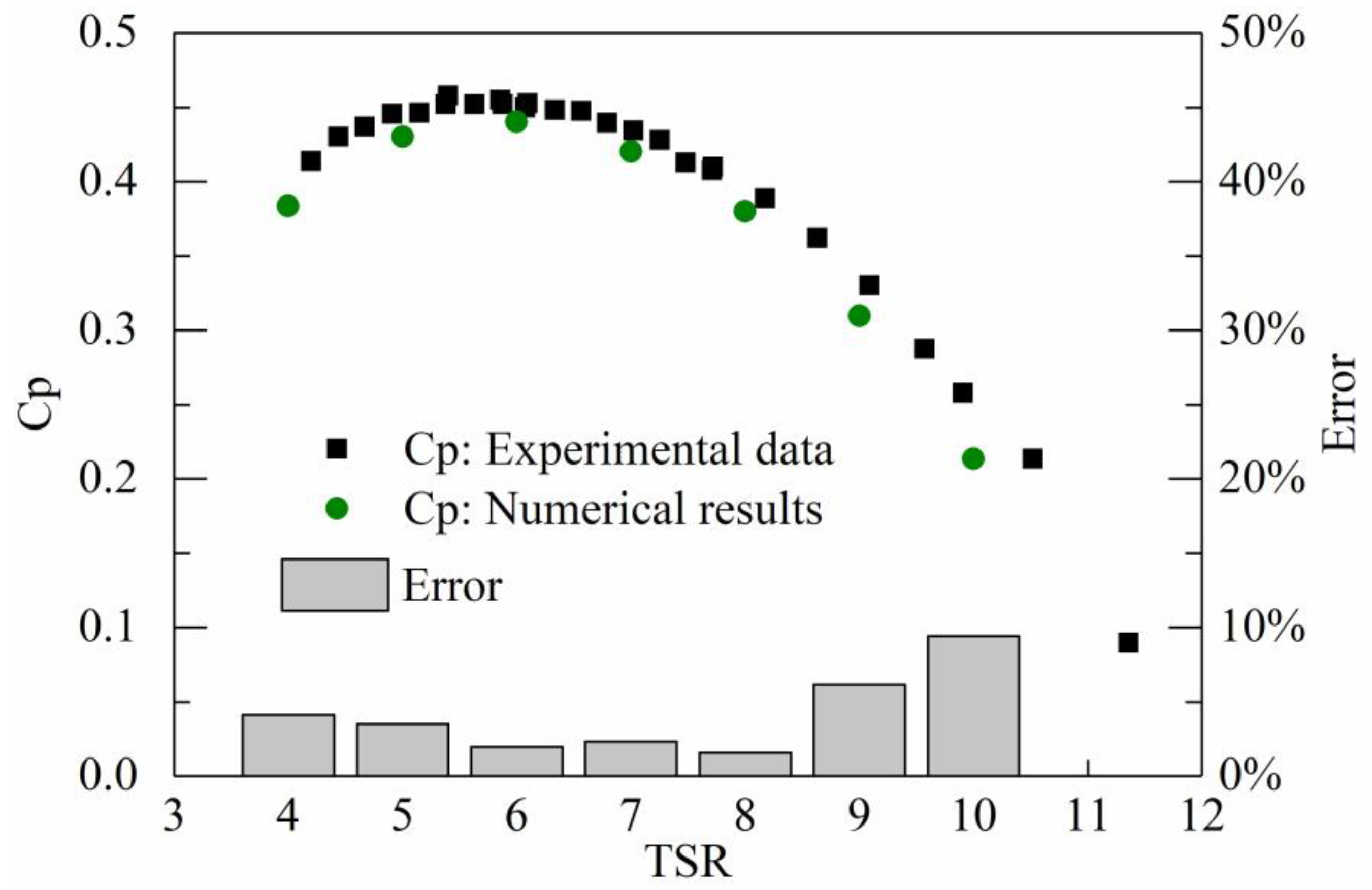
4. Numerical Method Verification and Validation

A mesh resolution study was carried out to evaluate the effect of mesh resolution on the torque of the HAHT and its coefficient of the power. The coefficient of the power is calculated as follows

$$C_p=\frac{M\omega }{0.5\pi r^2\rho v^3}$$

(24)

where $C_p$ is coefficient of the power, $M$ is the torque of the HAHT, and $\omega$ is the angular velocity of the HAHT. The results with different mesh resolutions are summarized in

Table 2. Results of torque and power coefficient for mesh verification.

Approx. Number of Grid Elements (million)	Torque/Nm	Cp
9.33	6.6872	0.3949
12.76	6.7939	0.4012
15.81	6.7972	0.4014

. It is seen that three different kinds of mesh configurations were investigated. The main different settings for the mesh generation were as follows: Mesh 1 had 15 layers of prisms applied on the surface of the blades, and the element size in the rotating flow domain was 1.5 mm; Mesh 2 had 20 layers of prisms and a 1.0-mm element size in the rotating flow domain; while Mesh 3 had 25 layers of prisms and a 0.8-mm element size in the rotating flow domain. It can be seen that Mesh 2 and Mesh 3 had approximately the same results, which indicates that further increasing the mesh resolution would not significantly affect the results of the torque and coefficient of power. Considering the economy of time, the mesh configuration of Mesh 2 was chosen in the following simulations.

Unfortunately, there are no published results for the noise validation of the horizontal axis hydrokinetic turbine considered in this study, but the hydrodynamic results for this case are available. To confirm the accuracy of the present simulation, the coefficient of power was compared with the experimental data of Bahaj et al. [33].

In the experimental test, a three-blade marine current turbine with 800 mm in diameter was tested in a 2.4 m × 1.2 m cavitation tunnel and a 60 m towing tank. The blades of the turbines were developed from the profile shape of NACA 63-8XX. The inflow velocity of 1.73 m/s was chosen to be compared with. The experimental results provided a series of results with a TSR from 4.1 to 11.3, and the TSR of integers from 4 to 10 were simulated by the LES method to investigate the torque output. Figure 6 shows the comparison of the coefficient of power between the present LES model and the experimental tests [33]. It can be seen that the results of the two methods followed the same trend, and the relative errors were within 4% for the cases of TSR = 5, TSR = 6, TSR = 7, and TSR = 8. The errors seemed to be larger when TSR = 9 and TSR = 10. Overall, the comparison between the present LES method and the experimental result shows an acceptable accuracy for this LES computation.

5. Results and discussions

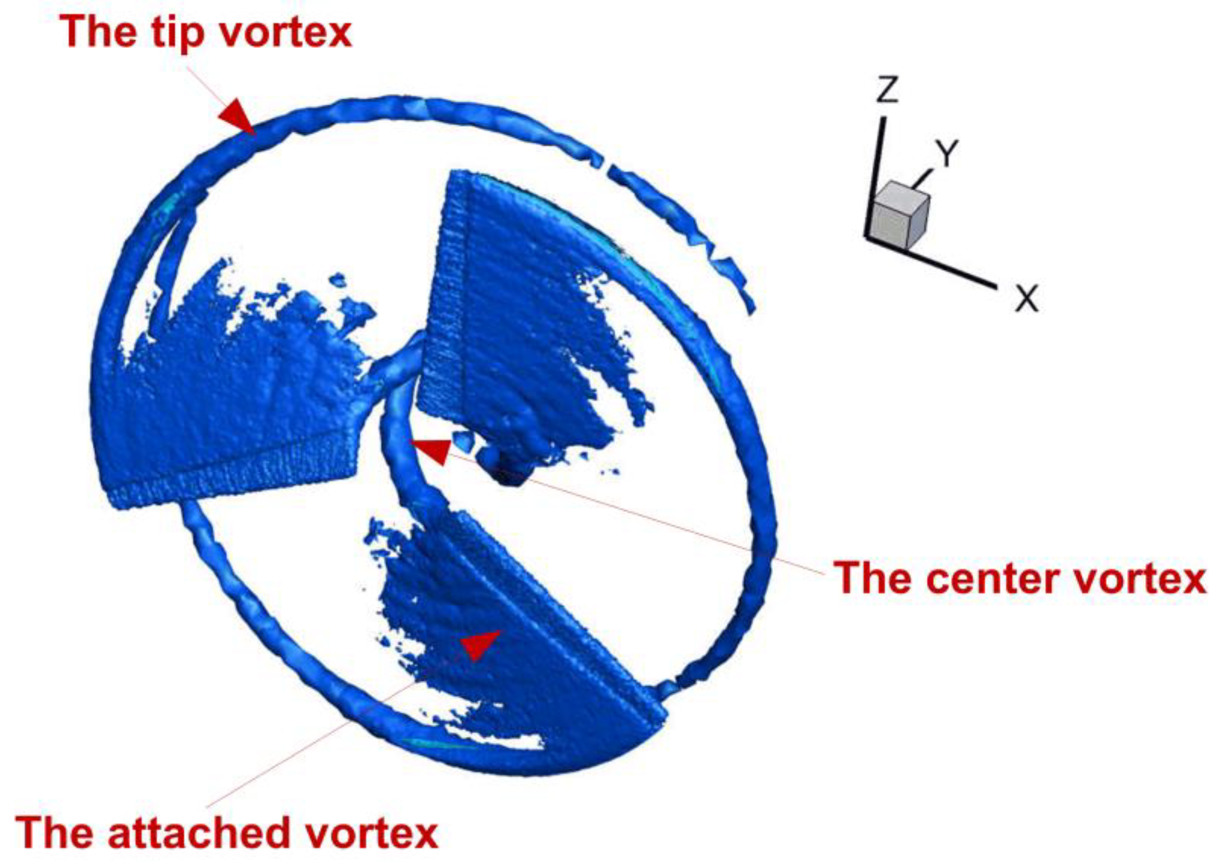
5.1. Flow Field Characteristics

The HAHT was designed for optimal efficiency at a constant revolution per minute (RPM) of 40, relating to the TSR of five at an incoming flow of 0.5 m/s. Therefore, the noise characteristics of the HAHT working at TSR = 5 were investigated preliminarily. To complete the numerical simulations, the material properties of the water utilized in the analysis are given in

Table 3. Material properties of water adopted in this paper.

Description	Parameter and Value
Temperature	$T$ = 20 °C
Density	$\rho$ = 998.2 kg/m3
Viscosity	$\mu$ = 0.001003 kg/(m·s)
Acoustic speed	$v$ = 1483 m/s
Reference sound pressure	$p_{ref}$ = 1 × 10−6 Pa

.

After the LES computation, the vortices generated around the HAHT are shown in Figure 7. It can be seen that plenty of vortices were generated after the turbine when the turbine rotated. As the hydrodynamic noise was closely related to the pressure fluctuations in the flow field, the pressure distribution around the turbine had to be emphasized. To observe the pressure characteristics clearly, the pressure contours at several cross sections of the blade are given in Figure 8. In Figure 8, the pressure range of the five cross sections is identical. It can be seen that the pressure fluctuations were gradually becoming more serious with the increase of the spanwise length from a 20% span to 80% span. At the cross sections of the 100% span, the pressure fluctuations weakened for both the barotropic region (red areas) and the negative pressure region (blue areas). From the pressure contours of the five cross sections of the blade, it is noticeable that the maximum absolute values of the pressure concentrate on the region of the leading edge of the airfoil and the suction surface of the airfoil. Unlike the other four cross sections of the airfoil, the negative pressure region of the 100% span spread over the suction surface from the leading edge to the trailing edge. To better investigate the hydrodynamic noise of the blade of the HAHT designed for UUMPs, its noise characteristics were subsequently investigated.

5.2. Noise Characteristics Around a Single Blade

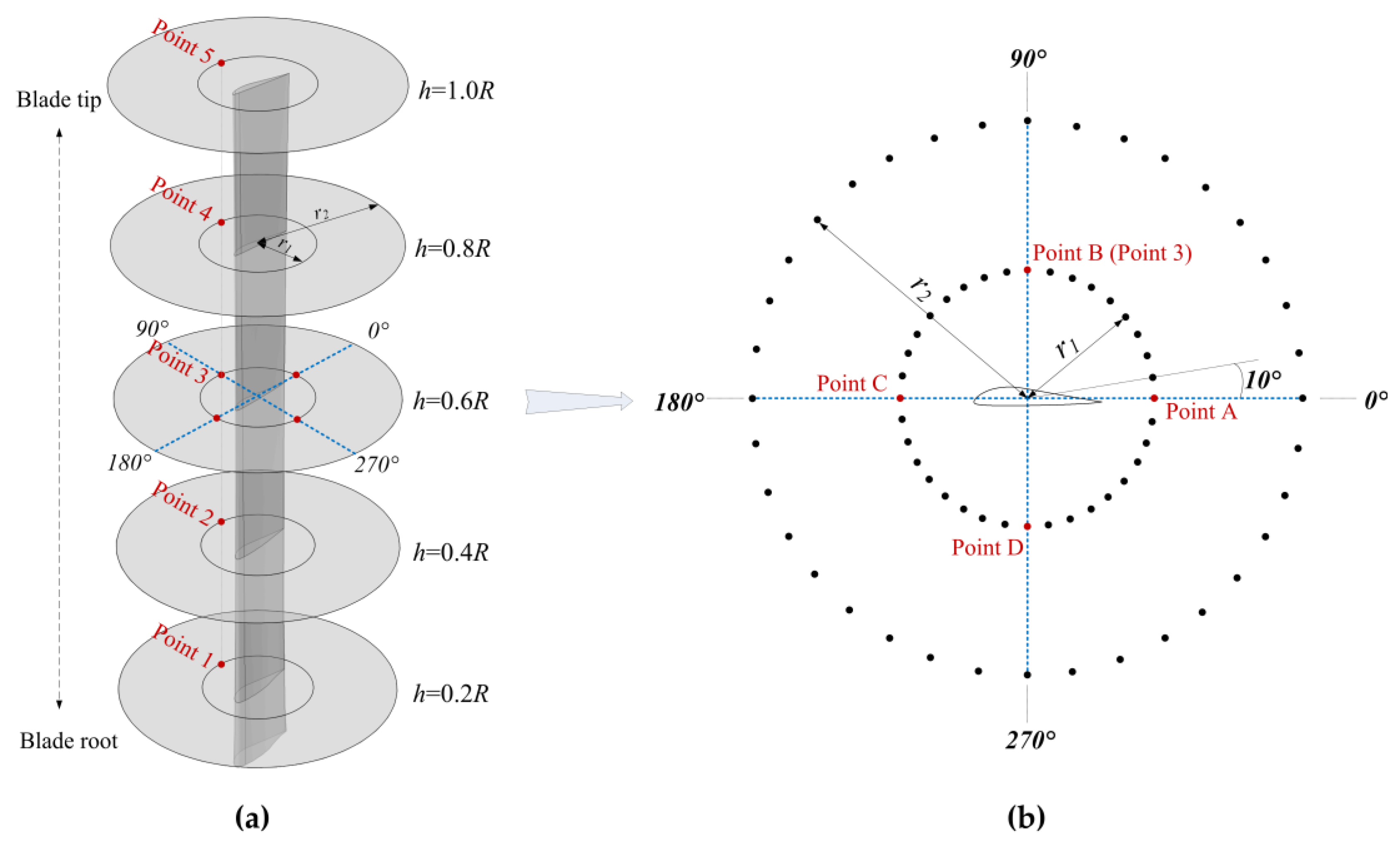
5.2.1. Arrangement of Noise Observation Location

First of all, the noise characteristics of a single blade were investigated. Figure 9 illustrates the noise observing points arrangement around a single blade. The acoustic monitoring points for the SPL computation were located at five different spanwise positions with h = 0.2 R, h = 0.4 R, h = 0.6 R, h = 0.8 R, and h = 1.0 R. For each spanwise position, there were two groups of observing points forming two circles with a radius r₁ = 40.0 mm and r₂ = 100.0 mm. The centers of the circles were at the aerodynamic center of the airfoil. For each circle, 36 acoustic monitoring points were distributed evenly with an interval of 10°. The direction of trailing edge of the airfoil was defined as 0°, the direction of the leading edge of the airfoil was defined as 180°, the direction of suction surface was 90°, and the direction of the pressure surface was 180°. To describe the noise spectrum of the monitoring points in a convenient way afterwards, the noise monitoring points at a 90° direction with radius r₁ were named Point 1, Point 2, Point 3, Point 4, and Point 5 at the five different spanwise positions. Additionally, the noise monitoring points at the spanwise position of h = 0.6 R with radius r₁ were named Point A, Point B, Point C, and Point D at directions of 0°, 90°, 180°, and 270°.

5.2.2. Results and Discussions of Noise Characteristics

The comparisons of the predicted OASPL of the single blade for noise observing points with different radii are shown in Figure 10. It can be observed that the OASPLs were gradually increasing from the spanwise location of 0.2 R to 0.8 R, except for the observing positions near the directions of 0° and 180°, while the overwhelming majority of noise observing points of the spanwise location of 1.0R had smaller OASPLs than the spanwise location of 0.8 R. It is seen from Figure 10 that the noise observing points with r₁ and r₂ had similar results. Combined with the results of Figure 8, it is understandable that the hydrodynamic noise was closely related to the pressure fluctuations near the surface of the turbine.

Figure 11 gives the comparisons of the predicted OASPL of the single blade for noise observing points at different cross sections. To observe the results clearly, the directions from 0° to 180° were chosen because of the almost symmetrical display. It can be easily seen that the OASPL of the observing points with a larger radius r₂ had smaller values than that of the observing points with a smaller radius r₁, except for the direction of 0° and 180°. Overall, the directionality of noise with different observing distances was identical.

Correspondingly, the predicted SPL spectra were analyzed. The predicted SPL spectra of Point A is shown in Figure 12. It can be easily seen that the high-value peaks were concentrated on the low frequency range, and there was broadband noise that existed after approximately 100 Hz. To exhibit the low-frequency peaks clearly, the frequency-axis was displayed in logarithmic form. It can be seen that the frequencies of the peaks were 2.0 Hz, 4.0 Hz, 6.0 Hz, 8.0 Hz, and so on, which can be calculated through the following expression:

$$f=\frac{knZ}{60}$$

(25)

where n is the speed of rotation (r/min); Z is the number of blades; k is positive integer (f represents the blade passing frequency (BPF) for k = 1, and f represents the higher order harmonics for k =2, 3, 4…). Thereafter, the following frequency-axis of the noise spectra as a function of frequency were all expressed in logarithmic form.

The comparisons of the predicted SPL of the single blade for noise observing points in different directions at the spanwise position of 0.6R are shown in Figure 13. It can be seen that the sound spectra were slightly different among the different directions. For the directions of 0° and 180°, there were more peaks compared with that of 90° and 270°. However, these different directions followed the same BPF and the same higher order harmonics. Among these four observing points, the OASPL of Point A was the largest, while the OASPL of Point D was the smallest. What is more, the comparisons of the predicted SPL of the single blade for noise observing points at different cross sections are plotted in Figure 14. It is noticeable that the observing position along the spanwise direction affected the noise characteristics a lot. At a 20% span, there were only two peaks at the frequency of the BPF and two times that of the BPF. With the increase in the spanwise length, the peaks became more and more abundant. As for the OASPL, it gradually increased with the increase in the spanwise length from Point 1 to Point 4; however, the OASPL of Point 5 was smaller than that of Point 4.

To explore the generation of the hydrodynamic noise essentially, the relationship between the flow field and the hydrodynamic noise field was further discussed. The hydrodynamic noise emission characteristics of a single blade were closely related to the pressure distributions near the surface of the turbine. It is obvious that the region near the blade had a higher OASPL value, and the value gradually increased from the blade root to the blade tip region. The maximal OASPL value was observed at the location between the blade root and the blade tip, which was closer to the blade tip region. From the point with a maximal OASPL value to the blade tip, the angle of the attack of the airfoil was extremely small, which resulted in the scatter and attenuation of the barotropic region and the negative pressure region. Thus, the OASPL at the 100% span of the blade become smaller. The noise spectra at the designated noise observing points showed that the maximum noise intensity can be obtained at 2.0 Hz, 4.0 Hz, and 6.0 Hz. The noise peak at the BPF was high, and peaks at the secondary and third frequencies were also high, which indicated that the hydrodynamic noise of the HAHT was mainly rotational noise.

5.3. Noise Characteristics Around the Whole Turbine

5.3.1. Arrangement of Noise Observation Location

The investigation of the noise characteristics around a single blade could provide a closer look into the noise generation near the surface of the blade. To investigate the noise emission characteristics of the HAHT designed for underwater mooring platforms, a group of noise observing points forming a spherical surface with radius of 6500.0 mm was chosen. Figure 15 shows the observing points’ arrangement around the whole turbine. The rotating center of the turbine was taken as the center of the sphere. The z-axis passed through the hydrodynamic centerline of one blade, and the y-axis, the flow direction, was the centerline of the UUMPs. There were 24 observing points evenly distributed along each circle, with an interval of 15°.

5.3.2. Results and Discussions of Noise Characteristics

As shown in Figure 16, p is an arbitrary observing point in the spherical surface with rotational center o of the three blades as the center of sphere, and line pp₁ is perpendicular to plane xoy at point p₁. The angle between line op₁ and the x-axis is defined as ${\alpha }_1$, and the angle between radius op and z-axis is defined as ${\alpha }_2$. For each observing point in the spherical surface, its position could be determined by the coordinate (${\alpha }_1$,${\alpha }_2$), where ${\alpha }_1$ = 0°, 15°, 30°, …, 345°, and ${\alpha }_2$ = 15°, 30°, 45°,…, 165°. After the FFT analysis, the OASPL of point p could be obtained. For the noise observing points in the spherical surface, the length of op was equal to the radius of the sphere. To investigate the directionality of the hydrodynamic noise produced by the HAHT, the length of op had to be proportionally transformed according to the value of OASPL with the direction (${\alpha }_1$,${\alpha }_2$) unchanged. The comparison of the predicted OASPL of the whole turbine for noise observing points in a spherical surface is shown in Figure 17.

It is seen from Figure 17 that there were obvious directionalities for noise transmission. It is noticeable that the dipole noise source dominated the sound sources in the current model. The noise was more likely to transmit along the flow direction (y-axis) than the x-axis direction and z-axis direction. To investigate the noise transmitted along the six directions of the three coordinate axes, including the x-axis (+), x-axis (−), y-axis (+), y-axis (−), z-axis (+), and z-axis (−), the comparison of the predicted OASPL is shown in Figure 18. It can be seen that the noise reduction rate along the y-axis was smaller than the noise reduction rate of the x-axis and z-axis. The comparisons of the cumulative sum of the sound power spectrum E(f) of the noise observing points along the x-axis and y-axis are exhibited in Figure 19, where f represents the frequency in the considered frequency range here. According to Wang [34], the cumulative sum of the sound power spectrum E(f) helps to identify major noise energy distributions in a way that is better than the more well-known SPL curve versus frequency, by observing the slope dE(f)/df. The cumulative sum of the sound power spectrum is defined as the integration from f = f₁ to f = f₂, expressed as follows:

$$\mathrm{E}(f)={\displaystyle {\mathsf{\int }}_{f_1}^{f_2}{p}^2}(f)\mathrm{d}f$$

(26)

It can be seen from Figure 19 that the major noise energies were all concentrated in a low frequency range (within 10.0 Hz). With the observing distance from 1000.0 mm to 6000.0 mm, the range of E(f) along the y-axis was from 1e-4 to 1; however, the smallest E(f) along the x-axis was lower than 1e-7, and its change range was wider. Therefore, the noise reduction degree along the x-axis was larger in the observing distance from 1000.0 mm to 6000.0 mm, which shows that the directionality of the noise emission of the HAHT was obvious. For researchers dealing with the noise study of the HAHT, the flow direction (y-axis) had to be emphasized because of the larger noise pressure levels compared with the other directions.

For the noise emissions around the whole turbine, the dipole noise source dominated the noise sources for the noise observing points, forming a circle parallel to the xoy surface. For each circle, the maximum OASPL could be obtained in the y-axis direction. The noise emission pattern of the HAHT investigated in this paper had similar characteristics to the results of Wasala et al. [35], concentrating on horizontal axis wind turbines, which is one typical kind of rotating machinery in the region of renewable energy. It can be seen that the OASPL did not change linearly with the observing distance, which implied that doubling the noise observing distance did not result in halving the OASPL. The cumulative sum of the sound power spectra showed that the noise energy was concentrated at a low frequency range, which is in accordance with the noise SPL spectra with main noise peaks at BPF and the first several higher order harmonics.

6. Conclusions

As a renewable energy source, marine current energy has been paid increasing attention all over the world. However, the noise emission problem of the energy conversion devices cannot be ignored, and the hydrodynamic noise generated by the rotating turbine has been known to be the most important noise source. In this study, the noise characteristics of the HAHT designed for UUMPs are evaluated based on LES, combined with the FW–H equation. In general, the coefficient of power of the hydrokinetic turbine after the LES calculation shows good agreement with the experimental data at different TSRs, denoting that the present flow field model is capable of accurately simulating the flow field characteristics. After verifying and validating the numerical method, the flow field characteristics and the noise characteristics are investigated. The main conclusions from the perspective of flow field characteristics, single blade noise characteristics, and whole turbine noise characteristics are as follows:

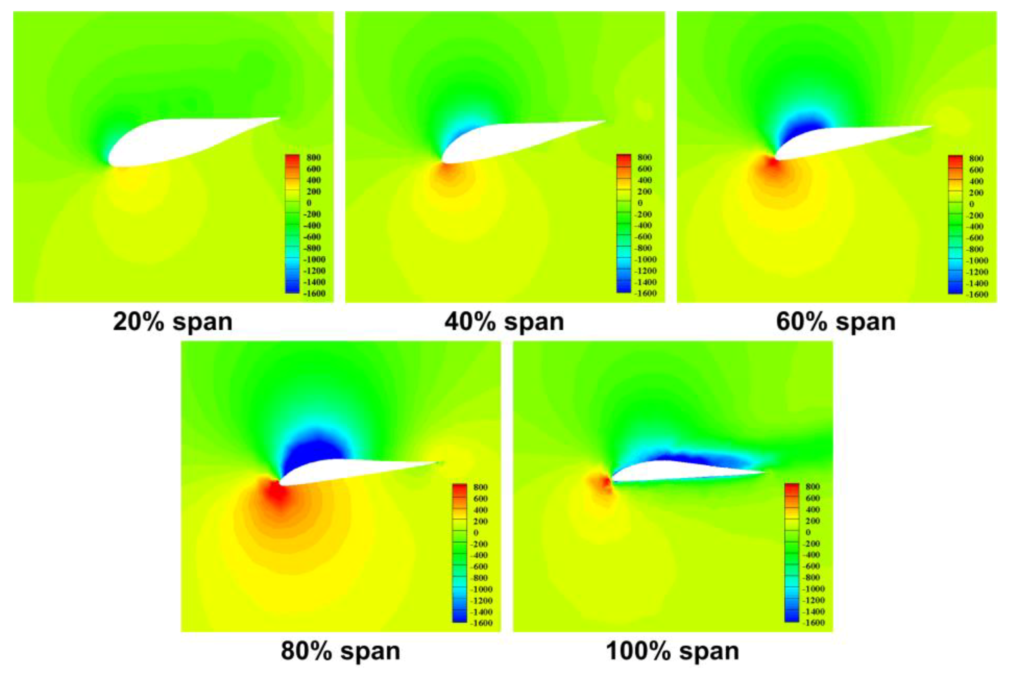
(1)

Along the spanwise direction of the blade, the pressure fluctuations are gradually becoming serious, with the increase of spanwise length from 20% span to 80% span. What is more, it is noticeable that the pressure fluctuations are concentrated in the region of the leading edge of the airfoil and the suction surface of the airfoil. With the increase in spanwise length, the negative pressure region gradually moves from the leading edge to the trailing edge on the suction pressure surface.

(2)

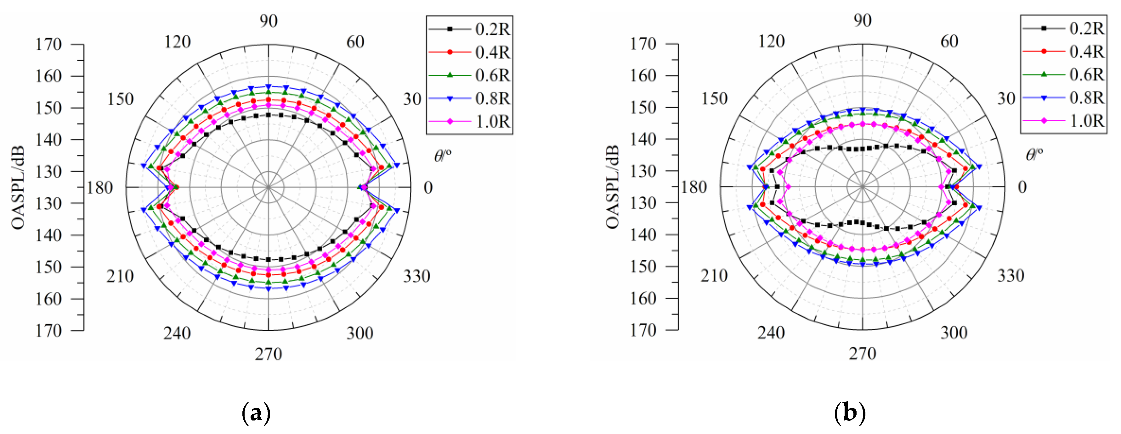
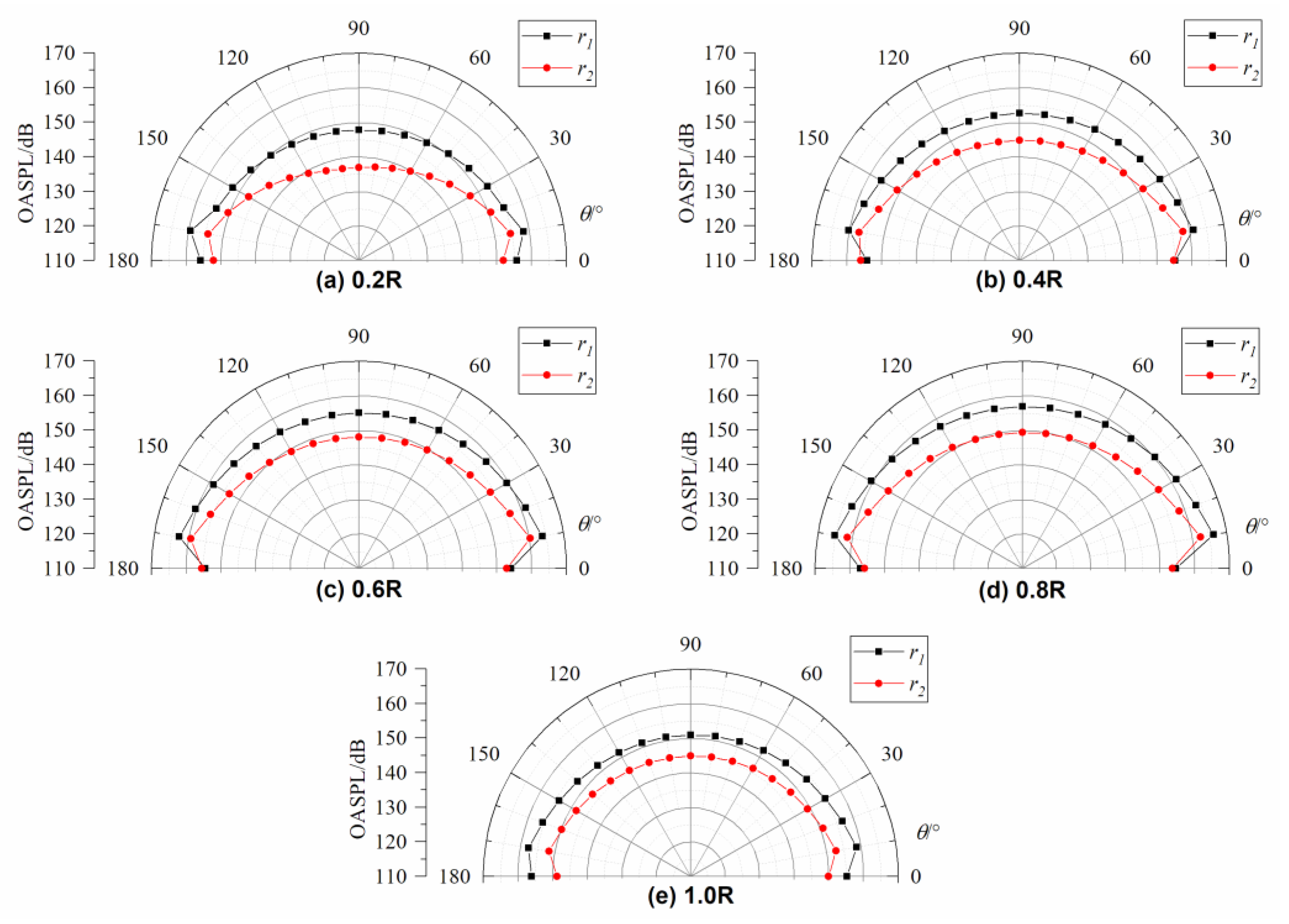
From the OASPL directionality around a single blade, it can be seen that the overall noise level of the spanwise location of 0.8 R has largest OASPL than that of the other spanwise locations in general, which is in accordance with the results of the flow field characteristics near the blade region. The sound spectra are slightly different among the different observing directions at the same spanwise location, and the observing location along the spanwise direction affects the noise spectra characteristics to a very great extent.

(3)

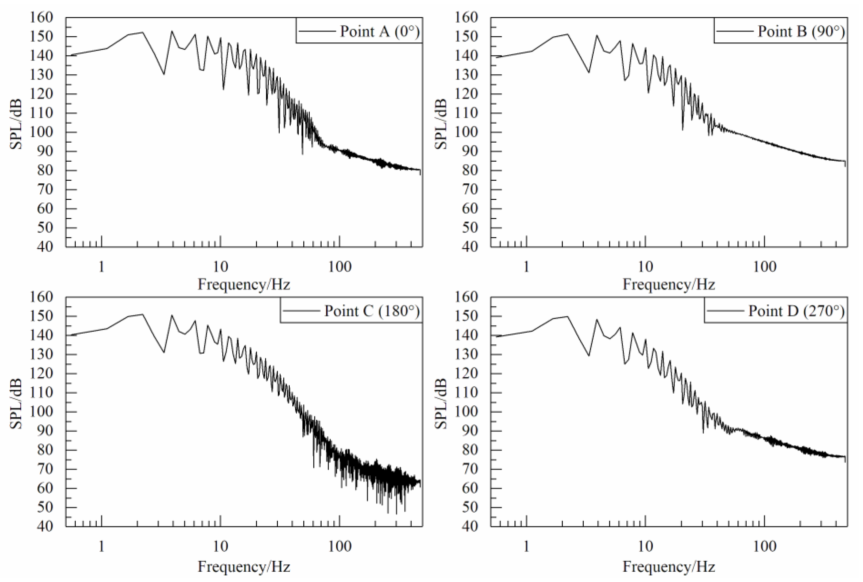
The investigation of the noise around the whole turbine indicates that the dipole noise source dominates the sound sources in the current analysis. The noise is more likely to transmit along the flow direction (y-axis in this paper) than the other directions. Furthermore, the cumulative sum of the sound power spectrum of the noise observing points along the x-axis and y-axis show the change relationship clearly.

In the present research, the HAHT is modeled as rotating about the fixed axis, and the interaction movement between the UUMPs is ignored. Therefore, further studies still need to be carried out on the following issues:

First of all, the effect of the interaction movement of the UUMPs on noise performance should be carried out. In actual working conditions, the UUMPs will move back and forth with the current; thus, more complex working environment and boundary conditions of the UUMPs and HAHT have to be conducted.

Secondly, the noise reduction design will be carried out according to the noise results around a single blade. Among the present noise reduction technologies of the turbines, the most suitable technology has to be determined with the modification of the blade.

Additionally, the experimental test of the noise performance of the HAHT designed for the UUMPs has to be carried out.

References

- Webb, D.C.; Simonetti, P.J.; Jones, C.P. SLOCUM: An underwater glider propelled by environmental energy. IEEE J. Ocean. Eng. 2001, 26, 447–452. [Google Scholar] [CrossRef]
- Crimmins, D.M.; Patty, C.T.; Beliard, M.A.; Baker, J.; Jalbert, J.C.; Komerska, R.J.; Chappell, S.G.; Blidberg, D.R. Long-endurance test results of the solar-powered AUV system. In Proceedings of the IEEE Oceans, Boston, MA, USA, 18–21 September 2006; pp. 1–5. [Google Scholar]
- Hine, R.; Willcox, S.; Hine, G.; Richardson, T. The wave glider: A wave-powered autonomous marine vehicle. In Proceedings of the IEEE Oceans, Biloxi, MS, USA, 26–29 October 2009; pp. 1–6. [Google Scholar]
- Tian, W.; Song, B.; Mao, Z. Conceptual design and numerical simulations of a vertical axis water turbine used for underwater mooring platforms. Int. J. Nav. Arch. Ocean 2013, 5, 625–634. [Google Scholar]
- Tian, W.; Song, B.; VanZwieten, J.H.; Pyakurel, P.; Li, Y. Numerical simulations of a horizontal axis water turbine designed for underwater mooring platforms. Int. J. Nav. Arch. Ocean 2016, 8, 73–82. [Google Scholar] [CrossRef] [Green Version]
- Sood, M.; Singal, S.K. Development of hydrokinetic energy technology: A review. Int. J. Energy Res. 2019, 43, 5552–5571. [Google Scholar] [CrossRef]
- Tian, W.; VanZwieten, J.H.; Pyakurel, P.; Li, Y. Influences of yaw angle and turbulence intensity on the performance of a 20 kW in-stream hydrokinetic turbine. Energy 2016, 111, 104–116. [Google Scholar] [CrossRef] [Green Version]
- Tian, W.; Mao, Z.; Ding, H. Design, test and numerical simulation of a low-speed horizontal axis hydrokinetic turbine. Int. J. Nav. Arch. Ocean 2018, 10, 782–793. [Google Scholar] [CrossRef]
- Salvatore, F.; Sarichloo, Z.; Calcagni, D. Marine turbine hydrodynamics by a boundary element method with viscous flow correction. J. Mar. Sci. Eng. 2018, 6, 53. [Google Scholar] [CrossRef] [Green Version]
- Knight, B.; Freda, R.; Young, Y.; Maki, K. Coupling numerical methods and analytical models for ducted turbines to evaluate designs. J. Mar. Sci. Eng. 2018, 6, 43. [Google Scholar] [CrossRef] [Green Version]
- Struthers, D.P.; Gutowsky, L.F.; Enders, E.; Smokorowski, K.; Watkinson, D.; Bibeau, E.; Cooke, S.J. Evaluating riverine hydrokinetic turbine operations relative to the spatial ecology of wild fishes. J. Ecohydraul. 2017, 2, 53–67. [Google Scholar] [CrossRef]
- Piper, A.T.; Rosewarne, P.J.; Wright, R.M.; Kemp, P.S. The impact of an Archimedes screw hydropower turbine on fish migration in a lowland river. Ecol. Eng. 2018, 118, 31–42. [Google Scholar] [CrossRef]
- Schuchert, P.; Kregting, L.; Pritchard, D.; Savidge, G.; Elsäßer, B. Using coupled hydrodynamic biogeochemical models to predict the effects of tidal turbine arrays on phytoplankton dynamics. J. Mar. Sci. Eng. 2018, 6, 58. [Google Scholar] [CrossRef] [Green Version]
- Hafla, E.; Johnson, E.; Johnson, C.N.; Preston, L.; Aldridge, D.; Roberts, J.D. Modeling underwater noise propagation from marine hydrokinetic power devices through a time-domain, velocity-pressure solution. J. Acoust. Soc. Am. 2018, 143, 3242–3253. [Google Scholar] [CrossRef] [PubMed]
- Lossent, J.; Lejart, M.; Folegot, T.; Clorennec, D.; Di Iorio, L.; Gervaise, C. Underwater operational noise level emitted by a tidal current turbine and its potential impact on marine fauna. Mar. Pollut. Bull. 2018, 131, 323–334. [Google Scholar] [CrossRef] [PubMed]
- Pine, M.K.; Schmitt, P.; Culloch, R.M.; Lieber, L.; Kregting, L.T. Providing ecological context to anthropogenic subsea noise: Assessing listening space reductions of marine mammals from tidal energy devices. Renew. Sust. Energy Rev. 2019, 103, 49–57. [Google Scholar] [CrossRef] [Green Version]
- Shigetomi, A.; Murai, Y.; Tasaka, Y.; Takeda, Y. Interactive flow field around two Savonius turbines. Renew. Energy 2011, 36, 536–545. [Google Scholar] [CrossRef]
- Dang, Z.; Mao, Z.; Tian, W. Reduction of hydrodynamic noise of 3D hydrofoil with spanwise microgrooved surfaces inspired by sharkskin. J. Mar. Sci. Eng. 2019, 7, 136. [Google Scholar] [CrossRef] [Green Version]
- Gallo, P.; Fredianelli, L.; Palazzuoli, D.; Licitra, G.; Fidecaro, F. A procedure for the assessment of wind turbine noise. Appl. Acoust. 2016, 114, 213–217. [Google Scholar] [CrossRef]
- Fredianelli, L.; Gallo, P.; Licitra, G.; Carpita, S. Analytical assessment of wind turbine noise impact at receiver by means of residual noise determination without the wind farm shutdown. Noise Control Eng. J. 2017, 65, 417–433. [Google Scholar] [CrossRef]
- Jung, S.S.; Cheong, C.; Shin, S.H.; Cheung, W.S. Experimental identification of acoustic emission characteristics of large wind turbines with emphasis on infrasound and low-frequency noise. J. Korean Phys. Soc. 2008, 53, 1897–1905. [Google Scholar] [CrossRef]
- Doolan, C. A review of wind turbine noise perception, annoyance and low frequency emission. Wind Eng. 2013, 37, 97–104. [Google Scholar] [CrossRef]
- Leloudas, G.; Zhu, W.J.; Sørensen, J.N.; Shen, W.Z.; Hjort, S. Prediction and reduction of noise from a 2.3 MW wind turbine. J. Phys. Conf. Ser. 2007, 75, 012083. [Google Scholar] [CrossRef]
- Ghasemian, M.; Nejat, A. Aero-acoustics prediction of a vertical axis wind turbine using Large Eddy Simulation and acoustic analogy. Energy 2015, 88, 711–717. [Google Scholar] [CrossRef]
- UIUC Airfoil Coordinates Database. Available online: https://m-selig.ae.illinois.edu/ads/coord_database.html (accessed on 31 October 2019).
- Hinze, J.O. Turbulence; McGraw-Hill Inc.: New York, NY, USA, 1975. [Google Scholar]
- Lighthill, M.J. On sound generated aerodynamically I. General theory. Proc. R. Soc. Lond. Ser. A 1952, 211, 564–587. [Google Scholar]
- Williams, J.F.; Hawkings, D.L. Theory relating to the noise of rotating machinery. J. Sound Vib. 1969, 10, 10–21. [Google Scholar] [CrossRef]
- ANSYS. ANSYS FLUENT Theory Guide; ANSYS Inc.: Canonsburg, PA, USA, 2011. [Google Scholar]
- Ffowcs, J.E.; Hawkings, D.L. Sound generation by turbulence and surfaces in arbitrary motion. Philos. Trans. R. Soc. A Math. Phys. Sci. 1969, 264, 321–342. [Google Scholar]
- Farassat, F. Derivation of Formulations 1 and 1A of Farassat; NASA Technical Report TM-2007-214853; NASA Langley Research Center: Hampton, VA, USA, 2007.
- Wang, S.; Yuan, P.; Li, D.; Jiao, Y. An overview of ocean renewable energy in China. Renew. Sust. Energy Rev. 2011, 15, 91–111. [Google Scholar] [CrossRef]
- Bahaj, A.S.; Molland, A.F.; Chaplin, J.R.; Batten, W.M.J. Power and thrust measurements of marine current turbines under various hydrodynamic flow conditions in a cavitation tunnel and a towing tank. Renew. Energy 2007, 32, 407–426. [Google Scholar] [CrossRef]
- Wang, C. Noise Source Analysis and Control for Small Axial-Flow Fans. Ph.D. Thesis, The University of Hong Kong, Hong Kong, China, 2016. [Google Scholar]
- Wasala, S.H.; Storey, R.C.; Norris, S.E.; Cater, J.E. Aeroacoustic noise prediction for wind turbines using Large Eddy Simulation. J. Wind Eng. Ind. Aerod. 2015, 145, 17–29. [Google Scholar] [CrossRef]