Synergistic Use of Synthetic Aperture Radar and Optical Imagery to Monitor Surface Accumulation of Cyanobacteria in the Curonian Lagoon

Abstract

Phytoplankton blooms in internal water bodies are an unpleasant sight that often emerges on top like a layer of foam containing high concentrations of toxins (scum event). Monitoring the concentration of algae and the occurrence of scum in lakes and lagoons has become a topic of interest for management and science. Optical remote sensing is a validated tool but unfortunately it is highly hindered by clouds. For regions with frequent cloud cover, such as the Baltic region, this means loss of data, which limits the purpose of sensing to spatially and temporally characterize any scum for a comprehensive ecological analysis. The aim of this paper is to investigate whether the use of synthetic aperture radar (SAR) images can compensate for the weaknesses of optical images for cyanobacteria bloom monitoring purposes in the event of cloudy skies. A “ready to use” approach to detect cyanobacteria bloom in the Curonian Lagoon based on the level 2 ocean product of Sentinel-1 images is proposed. This method is empirically validated for the images of summer/autumn 2018 of the Curonian Lagoon.

1. Introduction

Cyanobacteria, also known as blue-green algae, are aquatic bacteria affecting inland and coastal communities around the world and are some of the oldest living organelles on the Earth. Cyanobacteria can be found in many different environments such as freshwater and marine ecosystems. A mature blue-green algae bloom often surfaces atop as a layer of scum which is an unpleasant sight with potentially serious economic and health-related impacts [1].

In recent years, blooms of cyanobacteria have been increasing in magnitude, frequency and in geographical spread, due to climate change and human activity [2]. Warmer temperatures indeed favor cyanobacteria that generally grow better at higher temperatures than do other phytoplankton species [3]. Moreover, the warmer is the water surface, the steepest is the vertical stratification of inland waters, with a consequent reduction of vertical mixing layer. Many cyanobacteria take advantage of these stratified conditions by forming intra-cellular gas vesicles, which make the cells buoyant and able to accumulate in dense surface blooms [4]. Furthermore, global warming has extended the optimal growth period since water column stratifies earlier in spring and destratifies later in autumn [5]. Therefore, on top of water temperature, factors like turbulence levels, nitrogen fixation, long day-light and the buoyant ability of cyanobacterial cells play their part in the occurrence of scums [6].

While further understanding of biological and physical growth dynamics of various algae species is still ongoing, water managers are interested in monitoring the state of lakes and lagoons to be able to raise a red flag in time. In-situ data is the most widely used data-set for monitoring inland water bodies such as lakes and canals. These data-sets provide highly accurate, precise and in depth information on the state of a location at a point in time but are limited to few local points and their maintenance often reduces the in-situ coverage of a water body.

Satellite data have the advantage of taking frequent in time acquisitions and of providing a full spatial coverage at a coarse level, which allows trend detection in space and time. The Copernicus program, through Sentinel satellites constellations, ensures free, full and open access Earth Observation data availability for at least 20 years to come. Continuous, large scale studies of inland water ecosystems, biogeochemical processes and essential climate change variables can be performed for the very first time and with a spatial resolution suitable even for small lakes. These studies have the potential to tackle global scientific issues and to be a resource of information for management purposes [7]. Among the satellites of the Sentinels constellation, the recently launched Sentinel-1 (S1), Sentinel-2 (S2) and Sentinel-3 (S3) have the potential to provide information on bio-optical and physical properties of the waters.

Optical remote sensing is a validated tool for sensing, monitoring and developing better understanding of the state phytoplankton blooms from inland for example, References [8,9,10], to oceanic waters for example, Reference [11], successful applications in different study areas such as the Baltic Sea for example, References [12,13,14,15].

However, it is highly hindered by clouds. For regions with frequent cloud cover (such as the Baltic region) this means lack of data, which derails the purpose of sensing and makes difficult to spatially and temporally characterize any scum for a comprehensive ecological analysis. Moreover, cloudy conditions often favor the growth and aggregation of cyanobacteria on the surface since the consequent light reduction leads the algae to have excess buoyancy [16]. Therefore, the lack of data becomes even more serious with respect to the monitoring and management of aquatic environments and understanding of ecological phenomena in progress [17,18].

The weaknesses of optical images for cyanobacteria bloom monitoring purposes in the event of cloudy skies could be compensated by Synthetic-aperture radar (SAR) observations given the ability of the microwaves radiation to penetrate through cloud cover independent of weather conditions. It is indeed expected that cyanobacterial blooms lead to significant attenuation of SAR signal since they act as a viscous lid covering the water surface. To assess whether and to what extent microwaves can detect scum events is the aim of the present study.

A first step in this direction has been made by Svejkoky and Shandley [19], which integrated AVHRR and ERS-1 data to analyze and interpret a specific phytoplankton bloom phenomenon verified in the coastal area of California. In particular, the authors exploited the finer SAR spatial resolution to better identify the spatial distribution of the bloom quantified from the optical image.

Thereafter, Bresciani et al. [20] observed a significant decrease of the SAR signal for high values of chlorophyll-a cyanobacteria concentration for a wind speed between 2 and 6 m/s, by using data gathered during the Envisat mission from optical (MERIS) and microwave (ASAR) synchronous sensors. These findings support the use of microwave remote sensing as an additional tool to increase the temporal coverage of optical sensors. However, the use of radar alone to monitor algal blooms would be challenging. Indeed it is in general difficult to distinguish whether the decrease of the SAR signal is created by algal blooms or by other causes without additional information. On the other hand, optical/SAR integration might help differentiate natural slicks from those caused by oil or human activity.

Unfortunately, with the end of the Envisat mission, synchronous acquisition of optical and microwaves images are not longer available making difficult to rigorously improve the methodology to detect cyanobacteria bloom from SAR. Therefore, this paper aims to propose a ready to use approach to assign the presence of cyanobacteria blooms on empirical basis by using the Level 2 (L2) product of the SAR satellite Sentinel 1.

A good candidate as case study for the application of the proposed approach is the Curonian Lagoon, located in the South-Eastern Baltic Sea region. Indeed, while S1-L2 products are generally available only for open ocean, the closeness of the lagoon to the Baltic Sea makes that an exception. Moreover, cyanobacteria blooms occurring in the Curonian Lagoon have been widely investigated with dedicated field campaigns [21] and the optical water properties of the Curonian Lagoon in the presence of cyanobacteria have been ascertained [22,23].

2. The Curonian Lagoon

The Curonian Lagoon is the largest European lagoon. It is a shallow water body situated in the southern part of the Baltic Sea with a total area of 1584 km², a mean depth of 3.8 m and a total volume of water approximately of 6.2 km³, see Figure 1.

The Curonian Lagoon is a highly dynamic and complex ecosystem with many interacting processes. It is an open system, influenced by the exchange of the fresh Nemunas river water and brackish water of the Baltic sea. Indeed, it is separated from the Baltic by a narrow stretch of sandy beaches and woodland (0.5–4.0 km wide) called the Curonian Spit and is connected to Baltic’s water thought the Klaipeda Strait. Water salinity in the northern part of the lagoon may fluctuate between 0.1–7 psu and is representatives of marine, brackish and fresh-water species live. The southern part is constantly freshwater and characterized by a relatively closed water circulation with lower current velocities, where the wind is the main driver [24,25].

Pollution from a combination of shipping, military and industrial sources is heavily affecting the Lagoon influencing local tourism and economics. Untreated sewage also have increased the pathogenic organisms loads [26]. Not surprisingly, fishing and bathing in the lagoon have declined significantly in modern times. Moreover, the Lagoon receives water from the River Nemunas, that together with agriculture and urban activities is a major sources of phosphorus (P) and nitrogen (N), contributing significantly to the eutrophication processes underway [27].

A peak of nutrient concentrations is generally observed in winter and early spring, in correspondence of diatom blooms (mainly Asterionella formosa, Aulacoseira islandica, Stephanodiscus spp., Diatoma spp.), which lead to a decreasing of nitrate concentrations. This phenomenon and the associated rapid regeneration of phosphorus compounds create a favorable environment for cyanobacteria blooms in terms of N/P ratio [28], mainly involving Aphanizomenon flos-aquae, Planktothrix sp. and Microcystis spp. The A. flos-aquae, the most dominant cyanobacteria, are one of those containing microscopic vesicles and therefore are able to regulate their buoyancy and to drive the accumulations on the water surface [18]. Starting from late June and early July and lasting until the end of October, cyanobacteria species regularly become prevalent during which time they can bloom intensively [29,30].

In addition to the exceptional availability of the second level products of Sentinel-1, the Curonian Lagoon is a perfect case study for this research because is highly hindered by clouds. The effective presence and impacts of clouds can be exploited from Mercury et al. [31], who built a composite of MODIS-Terra 2001–2011 providing the global percentage of cloudiness for the 10-year period. It is found that the Curonia Lagoon has an yearly cloud coverage of the 76%. This percentage reduce to the 64% in the summer time. These values are not too far from what observed in the present study, indeed among the 150 optical acquisitions in the time interval considered (summer-autumn 2018), 90 are cloud covered.

3. Materials and Methods

Satellite images of Sentinel missions acquired between July and October 2018 are considered for this study. The Sentinel missions are a group of five satellites part of the European Space Agency (ESA) Copernicus program, for the observation and monitoring of the Earth’s surface, and the development of operational applications for environmental monitoring. All data gathered by the Sentinel satellites are provided for free, full and open access to users. More specifically, data from three of the Sentinel missions are used in this study.

• Sentinel-1 (S1), operating all-weather, day and night and performing C-band synthetic aperture radar imaging, enabling them to acquire imagery regardless of weather condition with a spatial resolution of 10 m.
• Sentinel-2 (S2) with the on-board Multispectral Instrument (MSI) provides high-resolution optical imaging over land and coastal waters. It measures the Earth’s reflected radiance in 13 spectral bands, at visible and mid-infrared wavelengths and at various spatial resolutions (10, 20, 60 m).
• Sentinel-3 (S3) that makes use of multiple sensing instruments, of which data acquired by OLCI (Ocean and Land Colour Instrument) are used in this study. It is a medium-resolution imaging spectrometer with 21 spectral bands with wavelengths ranging from the optical to the near-infrared at approximately 300 m.

All of these missions consist of a constellation of two twin polar-orbiting satellites.

3.1. Optical Images (Sentinel-2/MSI and Sentinel-3/OLCI)

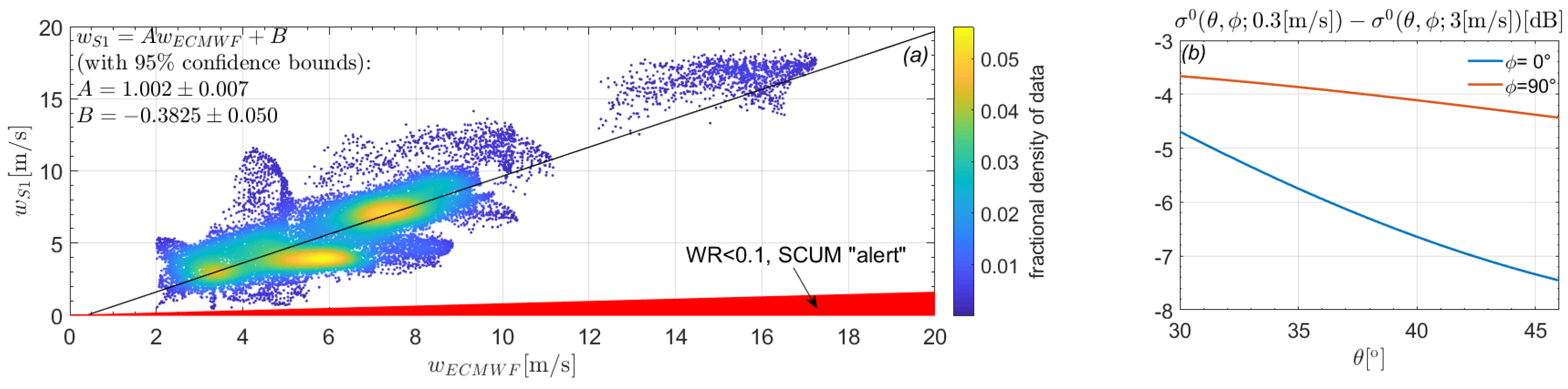
Within this study 33 S3/OLCI and 27 S2/MSI images acquired from July and October 2018 have been analyzed. The 60 optical images are analyzed to map chlorophyll a (Chl-a) concentrations using two different band ratio algorithms applied to atmospherically-corrected data. Given the very low transparency typical of the waters of the Curonian Lagoon [32] and the tendency of algae dispersed in the water column to accumulate near the surface, satellite-based estimates of Chl-a concentrations are presumably relevant only for the upper layer of water and thus can be considered as a proxy of the scum presence. Indeed the shallow, weakly stratified lagoon remains very turbid due to solids (mainly sand and silt) being resuspended as a result of water mixing caused by local winds and intensive primary production [33,34]. The Secchi disk depth varies from 0.3 to 2.2 m [29] and is always relatively low, so it is impossible to see the bottom at this shallow optical depth.

The atmospheric correction is carried out using the Second Simulation of the Satellite Signal in the Solar Spectrum-Vector code (6SV) [35] previously used in other satellite applications for the Curonian Lagoon [20]. The parametrization of 6SV code in case of the Curonian Lagoon is performed with Aerosol Optical Thickness (AOT) values gathered from AERONET station Gustav Dalen Tower located in the Baltic Sea and with water vapour values retrieved from daily MODIS products, via NASA Giovanni interface [36]. Chl-a concentration is produced after the application of a semi-empirical band-ratio model that uses the reflectance in the red and near-infrared (NIR) spectral regions [21,37]. The scum presence is calculated according to the approach by Bresciani et al. [20], with the ratio between reflectances in the near infrared (NIR) range. As indicated in INFORM D5.15 [38] (p. 140), Equation (1) is used for MSI

$$\text{Chl-a}\left[\frac{\mathrm{mg}}{{\mathrm{m}}^3}\right]=(76.36\pm 2.29)\frac{{\mathrm{Ref}}_{705}}{{\mathrm{Ref}}_{665}}-(51.57\pm 0.26),$$

(1)

and Equation (2) for OLCI

$$\text{Chl-a}\left[\frac{\mathrm{mg}}{{\mathrm{m}}^3}\right]=(52.19\pm 1.81)\frac{{\mathrm{Ref}}_{708}}{{\mathrm{Ref}}_{665}}-(32.07\pm 0.57),$$

(2)

where $Re{f}_x$ indicates the reflectance of the band with central wavelength x.

3.2. SAR Images

The Synthetic Aperture Radar (SAR) imagery, equipped with dedicated models and analysis tools, can provides information related to the water-surface, such as wind waves, currents, bathymetry, biological activity and precipitation. To first order, ocean SAR backscatter depends on the wind-generated short waves. Therefore, to estimate the wind-related impact on the SAR image is mandatory to interpret features such as the occurrence of phytoplankton bloom, oil spill, current fronts, surface eddies and others. In this purpose, ESA processes and delivers a Level-2 (L2) ocean product (OCN) designed to provide geophysical parameters related to wind, waves and surface velocity to the users. All acquisitions over the Curonia Lagoon are processed up the Level-2. The ocean wind component of the L2OCN product is available for all acquisition modes. For this study, only the geophysical parameters relied on L2OCN products acquired in interferometric wide (IW) swath mode are considered.

In the L2OCN product, the normalised radar cross section (NRCS) is used to derive the 10 m ocean surface winds using the geophysical model (GMF) called CMOD-IFR2 [39]. Since SAR is a single fixed antenna instrument, it cannot estimate both wind speed and direction and some a priori wind information is needed. ESA takes the additional wind vector information from the ECMWF (European Centre for Medium-Range Weather Forecasts) atmospheric model. To retrieve the ocean surface wind, radar parameters (NRCS values, incidence angle and track angle) and the a priori wind information are combined into a Bayesian scheme, described by Kerbaol et al. [40]. Although SAR wind retrievals are available for VV and HH polarization, only VV related winds are used throughout the paper. Both the a priori ECMWF wind vector and the related SAR retrieved winds are stored in the L2OCN netcdf files.

This wind inversion procedure has been successfully validated and applied to open ocean images. However, less work has been carried out for closed or semi-enclosed water basins, like the Curonia Lagoon, where the geographical boundaries may affect air–sea processes and sea states and wind regimes are controlled by short temporal and spatial fetches.

Figure 2a shows the scatter-plot between the a priori wind velocity given by ECMWF, ${\mathrm{w}}_{ECMWF}$ and the related SAR retrieved wind velocity, ${\mathrm{w}}_{S1}$, for 35 S1 images between 1 May 2019 and 30 June 2019, when no scum events were observed. As the ${\mathrm{w}}_{S1}$ is processed from ${\mathrm{w}}_{ECMWF}$, these two velocities have to clearly be correlated by construction. However, in Figure 2a it is evident that other features can affect SAR backscatter to the first order. In this study we are not interested to investigate all these features but rather to discuss the impact of the presence of phytoplankton blooms on water surface.

In Bresciani et al. [20], it is shown that phytoplankton blooms at water surface acts as a viscous layer by reducing the gravity-capillarly waves generation and propagation. From the SAR sensor point of view, scum phenomena are characterized by a reduced backscattered energy. Indeed, a drastic decrease in the NRCS (with attenuation greater than 8–10 dB) for Chl-a concentrations higher than 50 $\mathrm{mg}/{\mathrm{m}}^3$ and wind speeds in the range of 2 to 6 m/s is observed. This NRCS attenuation in turn leads to a retrieved SAR wind speed significantly smaller in respect to the ECMWF a priori guess.

The L2OCN data displayed in Figure 2a refer to a data-set where no phytoplankton bloom (or ice) events have been registered and that is independent from the one considered in Section 4 for results interpretation.

Empirically a “scum alert” can be raised when the retrieved wind is lower than the worst case observed in a no-scum calibration data-set. This relation can be expressed as

$${\mathrm{w}}_{S1}<{\mathrm{w}}_{\mathrm{fit}}-{\mathrm{err}}_{max},$$

where

$${\mathrm{w}}_{\mathrm{fit}}=1.002{\mathrm{w}}_{ECMWF}-0.3825$$

is obtained by Gaussian fit as shown in Figure 2a and

$${\mathrm{err}}_{max}=max\left\{\frac{{\mathrm{w}}_{\mathrm{fit}}-{\mathrm{w}}_{S1}}{{\mathrm{w}}_{\mathrm{fit}}}\mathrm{s}.\mathrm{t}.{\mathrm{w}}_{S1}<{\mathrm{w}}_{\mathrm{fit}}\right\}.$$

Notice that condition ${\mathrm{w}}_{S1}<{\mathrm{w}}_{\mathrm{fit}}$ refines the range as only damping effects needs to be considered. For the data-set in Figure 2a, ${\mathrm{err}}_{max}=0.8993$.

Let us define the ratio

$$\mathrm{WR}=\frac{{\mathrm{w}}_{S1}}{{\mathrm{w}}_{ECMWF}}$$

(3)

to monitor phytoplankton bloom from SAR, where ${\mathrm{w}}_{S1}$ is the wind speed estimated from Sentinel 1 and ${\mathrm{w}}_{ECMWF}$ indicates the a-priori ECMWF wind speed. As mentioned before, there are different factors able to significantly damp the backscatter but the knowledge of the lagoon’s characteristics and the seasonality of the events allow us to attribute the smallness of WR most likely to the presence of cyanobacteria’s bloom at the water surface.

Defining an index that does not come directly from the amplitude of the SAR signal, but rather from a derived product such as the retrieved wind, is due to the strong dependence of the NRCS on the incidence angle $\theta$. In Figure 2b it is shown how the condition $\mathrm{WR}=0.1$ is read in term of ${\sigma }^0$ for incidence angle values characteristic of S1 images for the Curonian Lagoon ($\theta \in$ [30°, 46°]) and different wind blowing direction. The use of an ocean-backscatter model such as CMOD allows to simply remove the incidence-angle dependence of the ${\sigma }^0$ and therefore to enable the estimation of phytoplankton bloom statistics in SAR images.

The a priori wind velocity also sets the applicability limits of this approach: for ECMWF wind speed below 2 m/s a weak backscattering area is likely due to a lack of wind than to the presence of floating substance on water surface. Therefore, this method can not be applied when ${\mathrm{w}}_{\mathrm{ECMWF}}$ falls in this range.

4. Results

As mentioned in Section 1, given the lack of a continuous and dedicated field campaign and the unavailability of synchronous acquisition of optical and radar images, a rigorous validation for the proposed method cannot be performed. Indeed, the dependencies of cyanobacteria on solar radiation and on air temperature and their ability to consequently perform vertical migration via buoyancy regulation makes their concentration highly variable within the time span of a daily cycle [16,21,41]. It is however viable to assess whether and to what extent the condition WR < 0.1 can be adopted as “SCUM alert” in terms of qualitative interpretation.

4.1. Discussion

Figure 3 collects results of two days in which all three satellites have done an acquisition, showing from left to right the S3 Chl-a product, the S2 Chl-a product (whose validation is documented in EOMORES D5.3 [42]), the S1 WR index map and the spatial and temporal evolution of ECMWF reanalysis wind vector. Areas affected by cloud cover are masked out in Chl-a maps as well as in S1 images areas where $w_{\mathrm{ECMWF}}$ is lower than $2\mathrm{m}/\mathrm{s}$. Times are expressed in UTC (Coordinated Universal Time).

Given the unavailability of synchronous SAR/optical images and the absence of in-field measurements in conjunction with the S1 acquisition, this research is focused to investigate whether the “anomaly” observed in SAR wind retrieval is compatible with a spatio-temporal evolution of scum observed in optical images.

First line of Figure 3 refers to the 29 August 2018 and is an example of slow bloom evolution typical of calm or gentle wind conditions [16].

The area with Chl-a $\gtrsim 100\mathrm{mg}/{\mathrm{m}}^3$, where visible, remains almost unvaried in the time between S3 and S2 acquisition.

S1 image is acquired six hours later the S2 ones. The area colored in red in Figure 3c is a little wider and slightly shifted to East in respect to the high Chl-a concentration area observed in Figure 3a,b. It is reasonable to envision that the associated wind speed (≈1 m/s) is too low to transport the surface accumulation of cyanobacteria elsewhere too far in the lagoon but large enough to be responsible for a slight convection. Considering the wind direction during the afternoon, see orange arrows in panel Figure 3d, this convection should be eastward. Moreover, as shown in Bresciani et al. [41], Chl-a concentration tends to increase during the day, reaching a maximum at mid afternoon for calm weather condition. We can therefore conclude that the red area observed for the S1 afternoon image is overall compatible with the evolution of the Chl-a maps driven by vector spatio-temporal variation. These finding support the hypothesis that WR < 0.1 can indicates phytoplankton bloom.

Second line in Figure 3 refers to 10 October 2018 and is an example of medium wind strength—wind speed (≈3.5 m/s) is high enough to be able to transport the bloom on the water surface but not enough to increase the mixing layer depth and the turbulence level in the water column. Comparison between Chl-a products from S3/OLCI, panel (e) and S2/MSI, panel (f), highlights how the phenomenon can quickly evolve in less than two hours. WR map from S1, panel (g), shows an alert area consistent with a realistic spatio-temporal evolution of the high Chl-a concentration area observed from optical images and the whole day wind vector direction and intensity.

These results seem to overall support the usability of the proposed approach, that in turn would confirm the leading role of solar radiance and wind speed and direction for daily spatial distribution and accumulation of positively buoyant cyanobacteria as discussed in References [20,41].

In Figure 4, results from those days where acquisitions from S1 and S3 are available are shown. The first line refers to the 17 August 2018 and also presents a case where presumably bloom increases its area in the afternoon and moves accordingly with wind direction. Second line refer to the 18 October 2018 morning time. S3 indicates bloom area in the south-est region; WR map locate the alert area in a region that is almost congruent with that showed in panel (e) with no significant spatio-temporal evolution.

Figure 5 collects results of those days where acquisition from S1 and S2 are available. Behaviours similar to those showed above are observed. 9 September 2018 (first line) WR map suggests again a case of afternoon spreading of bloom covered area consistent with wind direction. 18 October 2018 (second line) S1 acquisition is in the early morning and identifies an alert area bigger than the bloom area observed from S2 image acquired 5 h later.

These results suggest that the proposed approach based on wind ratio point out areas where water surface is affected by some factor that during summer/autumn time, as long as wind speed is greater than 2 m/s, can reasonably be identified as cyanobacteria’s bloom. S1-WR product can therefore contribute to the spatial and temporal characterization of the phenomena in order to improve the ecological analysis.

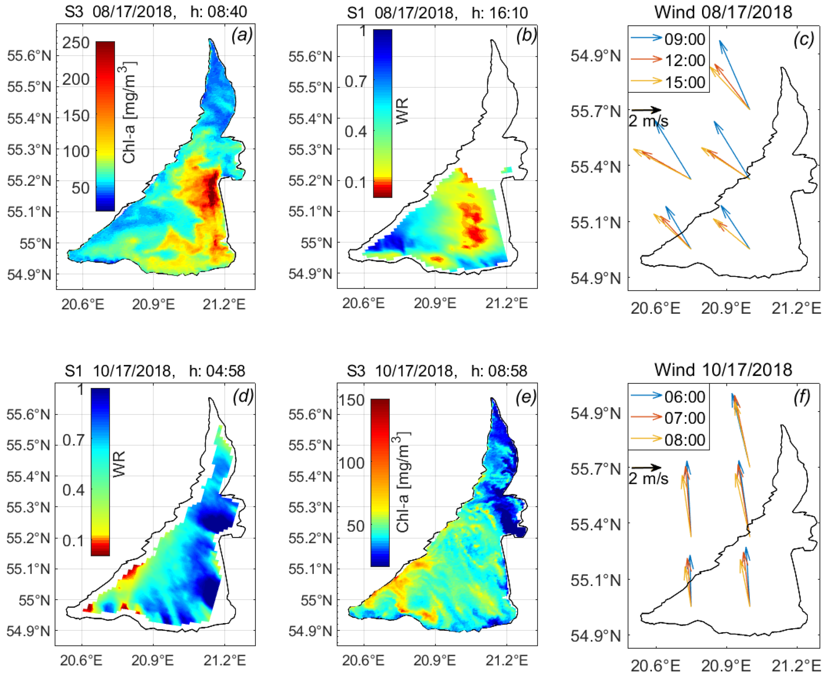
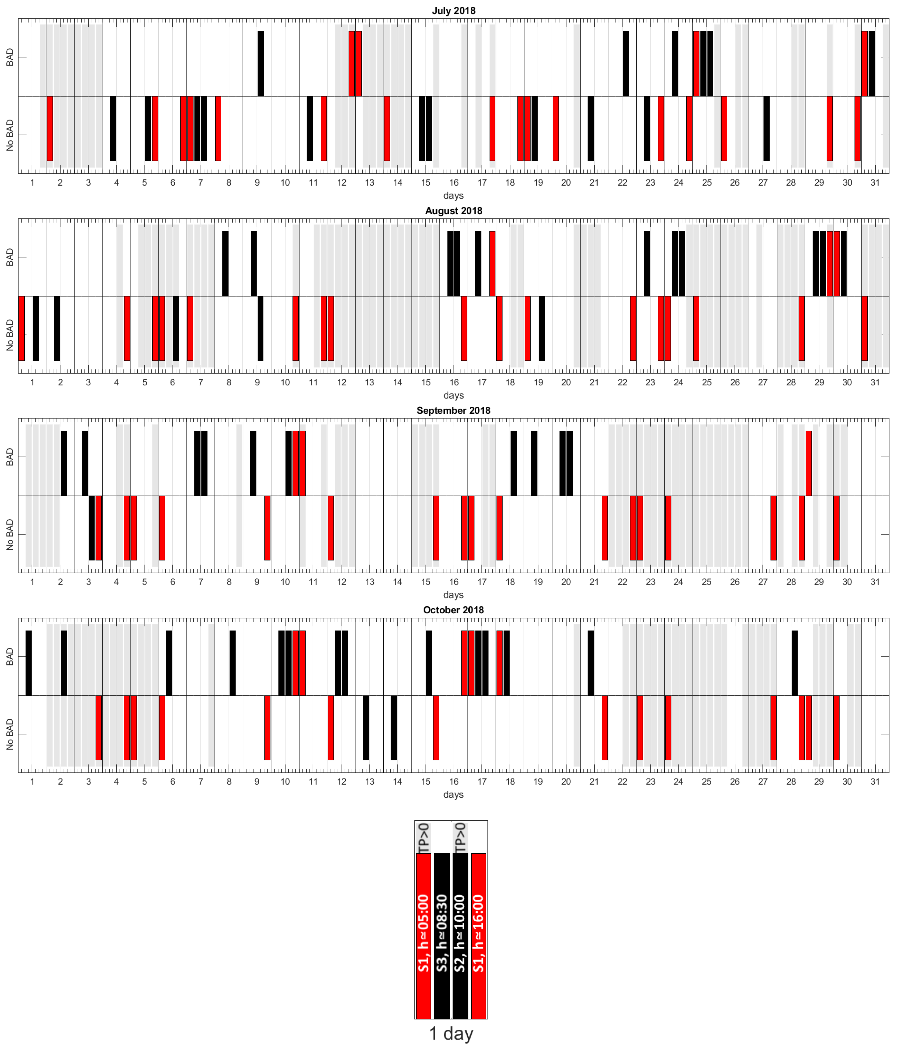
4.2. Application Example

An example of how the use of the proposed index could enrich a temporal characterization of the lagoon is shown in Figure 6. Let us recall that the main goal of the SAR based analysis here proposed consists in fill the gaps leaved by optical remote sensing techniques. This can be the case of no acquisition, of cloudy sky condition and of afternoon hours. As done in previous sub-section, we have thus to investigate whether wind ratio classification is compatible with the optical band ratio ones. Given the the large geographic extension of the lagoon and the wide window in which phytoplankton blooms can occurs, that is, almost 4 months, we propose hereafter the simplest and most synthetic approach for a temporal characterization of the lagoon.

Following the Water Framework Directive 2000/60/EC [43], the simplest temporal characterization of the lagoon can be performed classifying as “No BAD” images where Chl-a $<72\mathrm{mg}/{\mathrm{m}}^3$ in all the domain and as “BAD” any other. According to this paper’s hypothesis and the results showed above, the equivalent classification for S1 images corresponds to “No BAD” if $\mathrm{WR}>0.1$ everywhere in the lagoon and “BAD” otherwise.

Considering that C band radar can be additionally influenced by rain, the total precipitations time series is also showed for completeness. ERA5 hourly data on single level reanalysis database provides the total precipitation time series, represented in Figure 6 as gray background when is greater than zero. It seems that WR index based classification never gives false alarm caused by rainfalls. Indeed most of the days with precipitation and S1 acquisition are classified as “NO BAD” and the remaining cases are nearby other “BAD” classified images. This confirms that the WR index approach is actually self-sustained and that other meteorologic parameters are not needed.

Time series in Figure 6 again highlights that there would be a a significant lack of information due to the cloud cover if considering only optical data. Indeed, in this case there will be no data for the 62.2% of the days considered, of which the 67% can be recovered by integration through S1 results. Moreover even when optical data are available, SAR results can be used to evaluate the bloom persistence, as it happens for example on 08/29 and on 10/17.

Overall there are 28 days in which optical and SAR images are both acquired. Among these, in 16 days optical and SAR classify in the same way the lagoon; for the remaining 12 days some hypothesis can be formulated by distinguishing three different cases.

• SAR acquisition around 05:00 UTC classified as “No BAD” and optical images classified as “BAD”, this is the case of the 08/24, 09/18, 10/06 and 10/12.
  WR index seems still working reasonably since bloom typically forms later in the morning as the air temperature increases [41].
• Optical images classified as “BAD” and SAR acquisition around 16:00 classified as “No BAD”.

  -

  for the days 07/24, 08/23, 09/03, 10/15, 10/21 and 10/28 we observe that $w_{\mathrm{ECMWF}}>6$ m/s. Since the threshold wind speeds required for vertical mixing in shallow inland lakes typically goes from 3.1 m/s [44] to 4 m/s [45], it is therefore reasonable to assume that wind can produce shear forces on the water surface able to destabilize cyanobacteria’s buoyancy.

  -

  For the remaining two days (08/16 and 09/09) additional information is missing and it is difficult to understand if the WR index is failing or if bloom actually disappears for some unknown reason.

Summarizing, the SAR based approach returns a lagoon’s classification consistent with optical images results and meteorological data (high wind speed) for 22 cases, giving an agreement rate of the 79%. The different classification can the explained by the temporal acquisition gap for the 14% of the cases and solely the remaining 7% show a possible disagreement.

5. Conclusions

This paper proposes a “ready to use” approach to detect cyanobacteria bloom in the Curonian Lagoon based on the dependency between wind vector and radar backscatter. The open source and self-contained database of the level 2 ocean product Sentinel-1 images is considered. This method has been applied for Sentinel-1 images acquired in summer/autumn 2018. Qualitative comparison with optical imagery gathered from Sentinel-2 and Sentinel-3 satellites combined with meteorological data reveals that the method shows reasonable results for most of the analysed cases (the 79%). It presents the advantage to be an easy and self-sustained approach able to provide observations independently on the presence of atmospheric haze or cloud cover.

The presented findings strongly support the use of L2 S1 products to improve the spatio-temporal detection of algal bloom in Curonian Lagoon and complete the observations from optical sensors. Nonetheless, due to the unavailability of coincident pairs of SAR and optical imagery, a dedicated field observations could however refine the wind ratio threshold empirically determined in this paper. Overall, the combination of the three Sentinels (1, 2 and 3) is providing unprecedented observations in frequency and availability to water ecosystems studies concerned with trends and episodic events. The possibility of having multiple spatial scales (from 10 of S2 to 1 km of S1 L2 products) with different sensing time (from the earlier S3 to the later S1) finally support the understanding of cascade effect processes (e.g., cyanobacterial growth with scum formation), characterized by high degree of change and across a range of scales.

References

1. Paerl, H.W.; Paul, V.J. Climate change: Links to global expansion of harmful cyanobacteria. Water Res. 2012, 46, 1349–1363. [Google Scholar] [CrossRef]
2. Taranu, Z.E.; Gregory-Eaves, I.; Leavitt, P.R.; Bunting, L.; Buchaca, T.; Catalan, J.; Domaizon, I.; Guilizzoni, P.; Lami, A.; McGowan, S.; et al. Acceleration of cyanobacterial dominance in north temperate-subarctic lakes during the Anthropocene. Ecol. Lett. 2015, 18, 375–384. [Google Scholar] [CrossRef]
3. Reynolds, C.S. The Ecology of Phytoplankton; Cambridge University Press: Cambridge, UK, 2006. [Google Scholar]
4. Bartram, J.; Chorus, I. Toxic Cyanobacteria in Water: A Guide to Their Public Health Consequences, Monitoring and Management; CRC Press: Boca Raton, FL, USA, 1999. [Google Scholar]
5. PaeRL, H.; HussMann, J. Blooms like it hot. Science 2008, 320, 57–58. [Google Scholar] [CrossRef] [Green Version]
6. Walsby, A.E. Stratification by cyanobacteria in lakes: A dynamic buoyancy model indicates size limitations met by Planktothrix rubescens filaments. New Phytol. 2005, 168, 365–376. [Google Scholar] [CrossRef]
7. Tyler, A.N.; Hunter, P.D.; Spyrakos, E.; Groom, S.; Constantinescu, A.M.; Kitchen, J. Developments in Earth observation for the assessment and monitoring of inland, transitional, coastal and shelf-sea waters. Sci. Total Environ. 2016, 572, 1307–1321. [Google Scholar] [CrossRef] [Green Version]
8. Palmer, S.C.; Kutser, T.; Hunter, P.D. Remote sensing of inland waters: Challenges, progress and future directions. Remote Sens. Environ. 2015, 157, 1–8. [Google Scholar] [CrossRef] [Green Version]
9. Matthews, M.W. Eutrophication and cyanobacterial blooms in South African inland waters: 10 years of MERIS observations. Remote Sens. Environ. 2014, 155, 161–177. [Google Scholar] [CrossRef]
10. Bresciani, M.; Giardino, C.; Lauceri, R.; Matta, E.; Cazzaniga, I.; Pinardi, M.; Lami, A.; Austoni, M.; Viaggiu, E.; Congestri, R.; et al. Earth observation for monitoring and mapping of cyanobacteria blooms. Case studies on five Italian lakes. J. Limnol. 2017, 76. [Google Scholar] [CrossRef] [Green Version]
11. Bracher, A.; Vountas, M.; Dinter, T.; Burrows, J.; Röttgers, R.; Peeken, I. Observation of cyanobacteria and diatoms from space using Differential Optical Absorption Spectroscopy on SCIAMACHY data. In Proceedings of the 5th EGU General Assembly 2008, Vienna, Austria, 16 April 2008. [Google Scholar]
12. Kahru, M.; Elmgren, R. Multidecadal time series of satellite-detected accumulations of cyanobacteria in the Baltic Sea. Biogeosciences 2014, 11, 3619. [Google Scholar] [CrossRef] [Green Version]
13. Kutser, T.; Metsamaa, L.; Strömbeck, N.; Vahtmäe, E. Monitoring cyanobacterial blooms by satellite remote sensing. Estuar. Coast. Shelf Sci. 2006, 67, 303–312. [Google Scholar] [CrossRef]
14. Öberg, J. Cyanobacteria blooms in the Baltic Sea. In HELCOM Baltic Sea Environment Fact Sheets 2017; Helcom: Helsinki, Finland, 2016. [Google Scholar]
15. Reinart, A.; Kutser, T. Comparison of different satellite sensors in detecting cyanobacterial bloom events in the Baltic Sea. Remote Sens. Environ. 2006, 102, 74–85. [Google Scholar] [CrossRef]
16. Reynolds, C.; Walsby, A. Water-blooms. Biol. Rev. 1975, 50, 437–481. [Google Scholar] [CrossRef]
17. Bresciani, M.; Bolpagni, R.; Laini, A.; Matta, E.; Bartoli, M.; Giardino, C. Multitemporal analysis of algal blooms with MERIS images in a deep meromictic lake. Eur. J. Remote Sens. 2013, 46, 445–458. [Google Scholar] [CrossRef] [Green Version]
18. Walsby, A.E.; Ng, G.; Dunn, C.; Davis, P.A. Comparison of the depth where Planktothrix rubescens stratifies and the depth where the daily insolation supports its neutral buoyancy. New Phytol. 2004, 162, 133–145. [Google Scholar] [CrossRef]
19. Svejkovsky, J.; Shandley, J. Detection of offshore plankton blooms with AVHRR and SAR imagery. Int. J. Remote Sens. 2001, 22, 471–485. [Google Scholar] [CrossRef]
20. Bresciani, M.; Adamo, M.; De Carolis, G.; Matta, E.; Pasquariello, G.; Vaičiūtė, D.; Giardino, C. Monitoring blooms and surface accumulation of cyanobacteria in the Curonian Lagoon by combining MERIS and ASAR data. Remote Sens. Environ. 2014, 146, 124–135. [Google Scholar] [CrossRef]
21. Bartoli, M.; Zilius, M.; Bresciani, M.; Vaičiūtė, D.; Lubiene-Vybernaite, I.; Petkuviene, J.; Giordani, G.; Daunys, D.; Ruginis, T.; Benelli, S.; et al. Drivers of cyanobacterial blooms in a hypertrophic lagoon. Front. Mar. Sci. 2018, 5, 434. [Google Scholar] [CrossRef] [Green Version]
22. Bresciani, M.; Giardino, C.; Stroppiana, D.; Pilkaitytė, R.; Zilius, M.; Bartoli, M.; Razinkovas, A. Retrospective analysis of spatial and temporal variability of chlorophyll-a in the Curonian Lagoon. J. Coast. Conserv. 2012, 16, 511–519. [Google Scholar] [CrossRef]
23. Giardino, C.; Bresciani, M.; Pilkaityte, R.; Bartoli, M.; Razinkovas, A. In situ measurements and satellite remote sensing of case 2 waters: First results from the Curonian Lagoon. Oceanologia 2010, 52, 197–210. [Google Scholar] [CrossRef]
24. Ferrarin, C.; Razinkovas, A.; Gulbinskas, S.; Umgiesser, G.; Bliūdžiutė, L. Erratum to: Hydraulic regime-based zonation scheme of the Curonian Lagoon. Hydrobiologia 2010, 652, 397–397. [Google Scholar] [CrossRef] [Green Version]
25. Razinkovas, A.; Bliudziute, L.; Erturk, A.; Ferrarin, C.; Lindim, C.; Umgiesser, G.; Zemlys, P. Curonian lagoon: A modelling study-Lithuania. In Modeling Nutrient Loads and Response in River and Estuary Systems; Committee on the Challenges of Modern Society, North Atlantic Treaty Organization: Brussels, Belgium, 2005; pp. 194–222. [Google Scholar]
26. Kataržytė, M.; Mėžinė, J.; Vaičiūtė, D.; Liaugaudaitė, S.; Mukauskaitė, K.; Umgiesser, G.; Schernewski, G. Fecal contamination in shallow temperate estuarine lagoon: Source of the pollution and environmental factors. Mar. Pollut. Bull. 2018, 133, 762–772. [Google Scholar] [CrossRef] [PubMed]
27. Zilius, M.; Bartoli, M.; Bresciani, M.; Katarzyte, M.; Ruginis, T.; Petkuviene, J.; Lubiene, I.; Giardino, C.; Bukaveckas, P.A.; de Wit, R.; Razinkovas-Baziukas, A. Feedback Mechanisms Between Cyanobacterial Blooms, Transient Hypoxia, and Benthic Phosphorus Regeneration in Shallow Coastal Environments. Estuaries Coasts 2014, 37, 680–694. [Google Scholar] [CrossRef]
28. Pilkaitytė, R.; Razinkovas, A. Factors controlling phytoplankton blooms in a temperate estuary: Nutrient limitation and physical forcing. In Marine Biodiversity; Springer: Berlin/Heidelberg, Germany, 2006; pp. 41–48. [Google Scholar]
29. Gasiūnaitė, Z.R.; Daunys, D.; Olenin, S.; Razinkovas, A. The curonian lagoon. In Ecology of Baltic Coastal Waters; Springer: Berlin/Heidelberg, Germany, 2008; pp. 197–215. [Google Scholar]
30. Wasmund, N.; Nausch, G.; Gerth, M.; Busch, S.; Burmeister, C.; Hansen, R.; Sadkowiak, B. Extension of the growing season of phytoplankton in the western Baltic Sea in response to climate change. Mar. Ecol. Prog. Ser. 2019, 622, 1–16. [Google Scholar] [CrossRef] [Green Version]
31. Mercury, M.; Green, R.; Hook, S.; Oaida, B.; Wu, W.; Gunderson, A.; Chodas, M. Global cloud cover for assessment of optical satellite observation opportunities: A HyspIRI case study. Remote Sens. Environ. 2012, 126, 62–71. [Google Scholar] [CrossRef]
32. Vaičiūtė, D.; Bresciani, M.; Bartoli, M.; Giardino, C.; Bučas, M. Spatial and temporal distribution of coloured dissolved organic matter in a hypertrophic freshwater lagoon. J. Limnol. 2015, 74. [Google Scholar] [CrossRef] [Green Version]
33. Galkus, A. Vandens cirkuliacija ir erdvine drumstumo dinamika vasara Kuršių marių ir Baltijos jūros Lietuvos akvatorijose [Summer water circulation and spatial turbidity dynamics in the Lithuanian waters of Curonian lagoon and Baltic Sea]. Geogr. Metrašt 2003, 36, 3–16. [Google Scholar]
34. Mėžinė, J.; Ferrarin, C.; Vaičiūtė, D.; Idzelytė, R.; Zemlys, P.; Umgiesser, G. Sediment Transport Mechanisms in a Lagoon with High River Discharge and Sediment Loading. Water 2019, 11, 1970. [Google Scholar] [CrossRef] [Green Version]
35. Vermote, E.F.; Tanré, D.; Deuze, J.L.; Herman, M.; Morcette, J.J. Second simulation of the satellite signal in the solar spectrum, 6S: An overview. IEEE Trans. Geosci. Remote Sens. 1997, 35, 675–686. [Google Scholar] [CrossRef] [Green Version]
36. Available online: http://https://giovanni.gsfc.nasa.gov/giovanni/ (accessed on 12 December 2019).
37. Cazzaniga, I.; Bresciani, M.; Colombo, R.; Della Bella, V.; Padula, R.; Giardino, C. A comparison of Sentinel-3-OLCI and Sentinel-2-MSI-derived Chlorophyll-a maps for two large Italian lakes. Remote Sens. Lett. 2019, 10, 978–987. [Google Scholar] [CrossRef]
38. INFORM. INFORM Prototype/Algorithm Validation Report Update, D5.15. INFORM, 2016. Available online: https://www.google.com/url?sa=t&rct=j&q=&esrc=s&source=web&cd=1&ved=2ahUKEwjZnIq566_mAhW-UhUIHZEoBTUQFjAAegQIBBAC&url=http%3A%2F%2Finform.vgt.vito.be%2Ffiles%2Fdocuments%2FINFORM_D5.15_v1.0.pdf&usg=AOvVaw2S4Q_ofKQQBon-LYcm4a9_ (accessed on 12 December 2019).
39. Bentamy, A.; Queffeulou, P.; Quilfen, Y.; Katsaros, K. Ocean surface wind fields estimated from satellite active and passive microwave instruments. IEEE Trans. Geosci. Remote Sens. 1999, 37, 2469–2486. [Google Scholar] [CrossRef]
40. Kerbaol, V.; Wind, T.S.O.; Team, C. Improved Bayesian Wind Vector Retrieval Scheme Using ENVISAT ASAR Data: Principles and Validation Results. 2007. Available online: http://citeseerx.ist.psu.edu/viewdoc/summary?doi=10.1.1.434.4013 (accessed on 12 December 2019).
41. Bresciani, M.; Rossini, M.; Morabito, G.; Matta, E.; Pinardi, M.; Cogliati, S.; Julitta, T.; Colombo, R.; Braga, F.; Giardino, C. Analysis of within-and between-day chlorophyll-a dynamics in Mantua Superior Lake, with a continuous spectroradiometric measurement. Mar. Freshw. Res. 2013, 64, 303–316. [Google Scholar] [CrossRef]
42. EOMORES Consortium. D5.3 Final Validation Report. 2020; Under Review. Available online: https://eomores-h2020.eu/results/#deliverables (accessed on 12 December 2019).
43. Available online: https://eur-lex.europa.eu/eli/dir/2000/60/oj (accessed on 12 December 2019).
44. Cao, H.S.; Kong, F.X.; Luo, L.C.; Shi, X.L.; Yang, Z.; Zhang, X.F.; Tao, Y. Effects of wind and wind-induced waves on vertical phytoplankton distribution and surface blooms of Microcystis aeruginosa in Lake Taihu. J. Freshw. Ecol. 2006, 21, 231–238. [Google Scholar] [CrossRef]
45. Huang, C.; Li, Y.; Yang, H.; Sun, D.; Yu, Z.; Zhang, Z.; Chen, X.; Xu, L. Detection of algal bloom and factors influencing its formation in Taihu Lake from 2000 to 2011 by MODIS. Environ. Earth Sci. 2014, 71, 3705–3714. [Google Scholar] [CrossRef]
Figure 1. (a) Study area: the Curonian Lagoon; (b,c) examples of scum phenomena formed by cyanobacteria on the water surface of the Curonian Lagoon.
Jmse 07 00461 g001
Figure 2. (a) Scatter-density plot between the a-priori European Centre for Medium-Range Weather Forecasts (ECMWF) wind velocity, w E C M W F and the wind velocity estimated from Sentinel 1, w S 1 , from L2OCN products of internal points of the Curonian lagoon. Wind data showed are from 1 of May 2019 and 30 of June 2019, when no scum events were observed. The condition WR < 0.1, which sets empirically a “scum” alert, is colored in red ( R 2 = 0.72 , rmse = 1.7589); (b) Attenuation of the backscattering for WR = 0.1 as a function of the incidence angle θ . For data showed in panel (a), θ [30°, 46°]. Effect of wind direction ϕ is also showed, where ϕ = 0° corresponds to wind blowing towards the radar.
Jmse 07 00461 g002
Figure 3. Qualitative comparison between optical and radar products for single day acquisitions: Chl-a maps concentration derived from S3 (a,e) and from S2 (b,f); WR index maps from S1 (c,g); Top panels show results of 28 August 2018, bottom panels show results of 10 October 2018. (d,h) report wind vector spatiotemporal evolution during the time interval between acquisitions. Wind vector come from ERA5 hourly data on single levels reanalysis database.
Jmse 07 00461 g003
Figure 4. Qualitative comparison between S3 and S1 products for single day acquisitions: Chl-a maps concentration derived from S3 (a,e) and WR index maps from S1 (b,d); Top panels show results of the 17 August 2018, bottom panels show results of the 17 October 2018. Panels (c,f) report wind vector spatio-temporal evolution during the time interval between acquisitions. Wind vector come from ERA5 hourly data on single levels reanalysis database.
Jmse 07 00461 g004
Figure 5. Qualitative comparison between S2 and S1 products for single day acquisitions: Chl-a maps concentration derived from S2 (a,e) and WR index maps from S1 (b,d); Top panels show results of the 9 September 2018, bottom panels show results of the 18 October 2018; Panels (c,f) report wind vector spatio-temporal evolution during the time interval between acquisitions. Wind vector come from ERA5 hourly data on single levels reanalysis database.
Jmse 07 00461 g005
Figure 6. Temporal trends of WR (red bars), Chl-a concentrations (black bars) and Total Precipitation (TP) (gray bars) from July to October 2018. Images with Chl-a < 72 mg / m 3 or WR > 0.1 in all the domain are classified as “No BAD” [43]. Total Precipitation, indicated as a grey background when positive, come from ERA5 hourly data on single level reanalysis database and when is greater than zero is indicated as gray background. Temporal scheme is explained in the insert on the left.
Jmse 07 00461 g006