Hydrodynamic Zone of Influence Due to a Floating Structure in a Fjordal Estuary—Hood Canal Bridge Impact Assessment


Pacific Northwest National Laboratory, U.S. Department of Energy, Seattle, WA 98109, USA
*
Author to whom correspondence should be addressed.
J. Mar. Sci. Eng. 2018, 6(4), 119; https://doi.org/10.3390/jmse6040119
Submission received: 17 September 2018
/
Revised: 6 October 2018
/
Accepted: 10 October 2018
/
Published: 15 October 2018
(This article belongs to the Special Issue Selected Papers from the 15th Estuarine and Coastal Modeling Conference)
Abstract
:Floating structures such as barges and ships affect near-field hydrodynamics and create a zone of influence (ZOI). Extent of the ZOI is of particular interest due to potential obstruction to and impact on out-migrating juvenile fish. Here, we present an assessment of ZOI from Hood Canal (Floating) Bridge, located within the 110-km-long fjord-like Hood Canal sub-basin in the Salish Sea, Washington. A field data collection program allowed near-field validation of a three-dimensional hydrodynamic model of Hood Canal with the floating bridge section embedded. The results confirm that Hood Canal Bridge, with a draft of 4.6 m covering ~85% of the width of Hood Canal, obstructs the brackish outflow surface layer. This induces increased local mixing near the bridge, causes pooling of water (up-current) during ebb and flood, and results in shadow/sheltering of water (down-current). The change in ambient currents, salinity, and temperature is highest at the bridge location and reduces to background levels with distance from the bridge. The ZOI extends ~20 m below the surface and varies from 2–3 km for currents, from 2–4 km for salinity, and from 2–5 km for temperature before the deviations with the bridge drop to <10% relative to simulated background conditions without the bridge present.
1. Introduction
Hood Canal is a fjordal sub-basin within the Salish Sea region of Pacific Northwest. The Salish Sea is a collective name given to waterbodies that include the Strait of Juan de Fuca, Strait of Georgia, Puget Sound, and all their connecting channels and adjoining waters (see Figure 1). In the spring and summer, many Salish Sea sub-basins regularly experience algae blooms, and some of the sub-basins such as Hood Canal, East Sound, and regions of South Sound show signs of hypoxia [1]. Development of a comprehensive water-quality model of the Salish Sea was initiated in response to the above concerns about management of nutrient pollution and the assimilative capacity of the Salish Sea [2,3,4]. Of particular interest was the ability to simulate low dissolved oxygen (DO) events in the Salish Sea, including those responsible for fish kills and other chronic impacts in the Hood Canal region. Numerous studies were conducted in the past to determine what contributes to low DO events in Hood Canal, such as natural meteorological and oceanographic conditions, as well as anthropogenic causes, such as excessive nutrient loading [5,6].
The Hood Canal sub-basin includes a unique anthropogenic modification in that it hosts the Hood Canal Bridge (HCB), which is one of 11 floating bridges in use in the world. The geographic location of this 1992-m-long bridge, about 10 km from the mouth of Hood Canal, is indicated in Figure 1. Hood Canal is a 110-km-long narrow fjord-like sub-basin of Puget Sound with an average width of 2.4 km, a mean depth of 51.1 m, and a maximum depth of ~187 m, and it has a sill approximately 10–20 km from the mouth. The floating section of the bridge occupies ~85% of the width of Hood Canal, with a fixed opening at either end for small vessel traffic. The bridge has a design draft of 4.57 m. As part of the Salish Sea model development process, presence of the floating bridge was considered but not included in the model set-up under the assumption that effects of the bridge were likely a local phenomenon and unlikely to have a significant impact on the larger-scale Salish Sea model performance.
However, recent research suggests that the bridge may, in fact, alter hydrodynamics and has the potential to increase flushing time in Hood Canal. Circulation here exhibits classic fjord characteristics of a shallow brackish layer at the surface over a deep long and narrow saltwater column that is vulnerable to disruptions due to the presence of floating structures, which could constrict the mixing and transport in the upper layers of the water column [7]. Recent studies also indicate that the bridge is a barrier to fish passage. Slower migration times, higher mortality rates in the vicinity of the bridge relative to other areas on their migration route, and unique behavior and mortality patterns at the bridge suggest the bridge is impeding steelhead migration and increasing predation [8].
In this paper, we present an assessment of the near-field impact of the floating bridge on the tidal hydrodynamics in the Hood Canal fjord environment as a component of the Hood Canal Bridge Environmental Impact Assessment study [9]. In particular, we focus on quantifying the spatial extent of the change in hydrodynamic parameters, such as currents, salinity, and temperature, in the vicinity of the bridge relative to ambient conditions. This near-field region of deviation from ambient background is the zone of influence (ZOI), defined arbitrarily as the distance from the bridge where relative difference induced by the structures reduces to <10% of the maximum deviation. This was accomplished through an application of the Salish Sea model [4] with the HCB embedded in high resolution. We present a summary of field data collected at the bridge, set-up and calibration of the Salish Sea model with a floating bridge module, and application of the model to the development of quantitative estimates of ZOI dimensions. These results inform companion studies addressing the impacts on the swimming behavior and observed mortality of out-migrating juvenile steelhead at HCB. Although this study discusses site-specific efforts, the results and the concern about potential ecological impacts are applicable to all floating bridges worldwide.
2. Materials and Methods
2.1. Oceanographic Data Collection
Oceanographic data collection was planned with two objectives: (1) field confirmation of the hypothesis that the HCB obstructs and alters near-field surface currents; (2) provide near-bridge data for the calibration of hydrodynamic models. Near field, for the purpose of this scope, is defined as the region where the influence of the bridge on current, salinity, and temperature variables is noticeable relative to the ambient (far field). Based on a prior modeling effort [7], the ZOI was expected to vary from as small as one to two bridge widths (18–36 m) normal to the direction of flow, to a much larger region covering several Hood Canal channel widths (2.4–7.2 km), for variables such as currents, temperature, and salinity.
In situ current and conductivity, temperature, and depth (hereafter CTD) measurements were collected over a four-week period, from late April to early June 2017, at three locations near HCB [10]. Figure 2 shows the locations of the stations (a) immediately below the floating bridge span, (b) approximately 500 m upstream (south) of the bridge, and (c) approximately 500 m downstream (north) of the bridge. The bridge-mounted current meter (a) was attached to the floating section of the bridge. Attachment of the acoustic Doppler current profiler (ADCP) to this platform provided a profile of the water currents directly below the bridge. In addition to the ADCP, the bridge-mounted system also included a single-point Aquadopp current meter attached approximately 1 m below the hull of the bridge to collect in situ current data as close to the structure as feasible. The upstream and downstream deployment locations were constrained by the fact that they needed to be bottom-mounted (outside of marine traffic in the surface waters) and away from HCB mooring lines. Also, the maximum water depth at the bridge central span was ~101 m and posed a challenge for the upward-looking ADCP instrument’s ability to penetrate the surface layers. They were, therefore, deployed at a depth of approximately 50 m and as far from the shoreline as possible. Continuous CTD measurements were obtained from the bridge and bottom-mounted stations along with CTD casts during deployment and recovery.
2.2. The Salish Sea Model Set-Up
The Salish Sea model is an externally coupled hydrodynamic and biogeochemical model developed by the Pacific Northwest National Laboratory in collaboration with Washington State Department of Ecology to support coastal estuarine research, restoration planning, water-quality management, and climate-change response assessments in the region [2,3,4] The model was constructed using the unstructured grid Finite-Volume Community Ocean Model (FVCOM) [11] version 2.7 framework and integrated-compartment model biogeochemical water-quality kinetics [12,13]. To facilitate enhanced exchange with the Pacific Ocean, the Salish Sea model grid was expanded to include coastal waters around Vancouver Island and the continental shelf from Canada’s Queen Charlotte Strait to Oregon’s Waldport, south of Yaquina Bay [14]. The model kinetics were also improved through the addition of sediment diagenesis and carbonate chemistry [15], and it is capable of reproducing the observed biogeochemical conditions of the Salish Sea (salinity (S), temperature (T), dissolved oxygen (DO), nitrate, algal biomass, and pH), including near-bed hypoxia in key locations such as the Lynch Cove region of Hood Canal, Penn Cove, and East Sound [4].
Figure 3a shows the Salish Sea model domain and grid with 16,012 nodes and 25,019 triangular elements. The vertical configuration of the model uses 10 sigma-stretched layers distributed using a power law function with an exponent P-Sigma of 1.5, which provides more layer density near the surface. The model was set up for the year 2017 covering the near-field data collection period of April through June. The model is loaded with daily values of freshwater inflow from a total of 23 major gauged rivers, 46 ungauged streams for which flows were estimated through hydrological analysis, and 100 wastewater flows [16]. The model is forced with wind and heat flux at the water surface. Meteorological inputs were obtained from Weather Forecasting Research Model reanalysis data generated by the University of Washington. Tidal forcing at the open boundary was based on tidal constituents (S2, M2, N2, K2, K1, P1, O1, Q1, M4, and M6) derived from the Eastern North Pacific or ENPAC model [17]. Temperature and salinity profiles at the boundary were extracted from World Ocean Atlas 2013 version 2 [18,19] climatological fields of in situ temperature and salinity at a 1° grid interpolated to the model boundary nodes. Spin up for the hydrodynamic model was conducted through a one-year run initiated from stationary conditions (zero initial velocity and water surface elevation) with uniform T (7 °C) and S (32 practical salinity units (PSU)). The simulation was then repeated using year-end results as the restart initial condition.
As a preliminary step, Salish Sea model validation over the entire domain was first conducted to ensure that modification of the model grid and layering scheme (described in the following section) did not alter the overall model performance. This was done using year-long monitoring data available from a prior year (2014). The error statistics of water-surface elevation, S, and T were computed at nine tide stations and 24 water-quality stations maintained by Washington State Department of Ecology and shown in Figure 3b. Overall calibration results for T and S at all stations were found to be reasonable. Relative water-surface elevation errors were less than 10% at all stations within Puget Sound in United States (US) waters. Domain-wide T root-mean-square error (RMSE) was 0.94 °C with a bias of −0.03 °C. The domain-wide S error was 0.96 PSU with a bias of −0.24 PSU. Model skill scores were also high for T and S with Willmott skill score (WSS) [20] values of 0.96 and 0.80, respectively (see Table 1).
2.3. Hood Canal Bridge Module Implementation
The FVCOM framework used in the Salish Sea model is a three-dimensional, free-surface, terrain-following solver for the primitive form of Navier–Stokes equations. The model uses an unstructured grid in the horizontal dimension and sigma-stretched coordinate system in the vertical dimension. The floating bridge in this framework may be best approximated by a rectangular barge-like pontoon (see Figure 4 for HCB profile and cross-section details). However, representation of the rectilinear shape of the pontoons in this discretized framework requires special attention. While the width and the horizontal dimensions may be represented in a straightforward manner by suitable refinement and arrangement of the triangular elements, representing the uniform draft in a terrain-following sigma coordinate system poses a particular challenge. The dimensions of the bridge were specified as 1992 m long and 18.3 m wide, with a draft of 4.57 m. Figure 5 shows a close-up of the model grid refinement for the HCB region of the domain. The following three techniques were explored:
- (a)
- Implementation of a velocity block: This approach is identical to that described by Khangaonkar and Wang (2013) [7] where the impermeable surface block was incorporated into FVCOM with modification of both external and internal modes of the solver. For the baroclinic internal mode, the horizontal velocities at the selected cells and surface layers were always specified as zero such that no horizontal flow was allowed to pass through. During the barotropic external mode calculations, the cross-sectional water column depth at selected cells occupied by the block was adjusted to a new reduced value by subtracting the blocked layer thickness from the total water depth. This modification accommodates the presence of the rigid structure but is an approximation, as non-hydrostatic components of the pressure term, which are likely to be strong in the near field, are neglected. Effects of the bridge on momentum terms are addressed, but are done so as an indirect effect of setting the surface boundary to zero velocity without affecting the pressure term.
- (b)
- Implementation of momentum sink at the bridge using form drag: In this approach, the cells occupying the bridge are populated with hypothetical cylinders similar to a densely packed kelp farm. The drag from the cylinders set to sufficiently high value results in blockage of nearly ~95% of surface currents. Although this represents a leaking bridge, the implementation allows effects on continuity, as well as momentum, terms of the governing equations. The implementation of form drag from suspended cylinders in the water column was described by Wang et al. (2013) [21]. This method also requires local modification of the bathymetry to a representative average depth under the bridge for representation of the rectangular shape of the bridge pontoons.
- (c)
- Free surface pressure modification with a bottom drag: This method relies on modification of the free surface pressure boundary condition; an increase in pressure equivalent of 4.57 m of head results in a model response of 4.57 m depression of the free surface. This method is an improvement over (a) and (b) in that bathymetry is unaltered. In addition to modifying the free surface, the method also employs drag formulation for the layer immediately under the bridge. This results in flow passing the bridge under modified pressure with suitable reduction in velocity induced by the form drag.
The efficacy of each method was tested by examination of predicted velocity, temperature, and salinity profiles relative to the data collected. Results showed that all methods provided similar performance in terms of near-field impacts to the flow field. For simplicity, the continuity/velocity block method (a) was retained for the remainder of the analysis.
2.4. Near-Field Model Validation
The near-field model validation consisted of comparison of predicted water surface elevations, currents, salinity, and temperature results with data measurements during the 2017 field program.
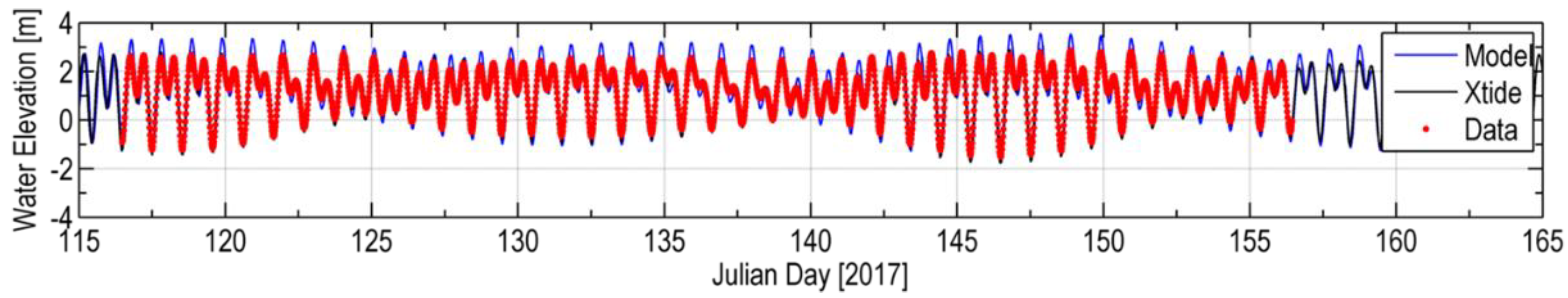
Water surface elevations: Water surface elevation measurements were collected at a station located on the east bank of Hood Canal. Figure 6 shows a comparison of measured data and water surface level simulated by the model. Absolute mean error (AME) or bias at this station was 0.013 m, and RMSE was 0.42 m, which is an error of 8% relative to the tidal range of 5.34 m (Table 2).
Salinity and temperature: In addition to velocity profiles, North ADCP, Bridge ADCP, and South ADCP stations also provided salinity and temperature data. Temperature and salinity data were measured at a depth of 1 m below the bridge hull (5.57 m depth) at the Bridge ADCP station, while at the North ADCP and South ADCP stations, these data were collected at a depth of ~50 m near the seabed. Figure 7 shows the time-series comparison of observed data and simulated salinity and temperature at the three ADCP locations. The salinity variation at the three ADCP stations was successfully reproduced in the model simulations. Predicted temperature variations were also in good agreement with observed data.
The error statistics (AME and RMSE) between model predictions and field observations are listed in Table 3. The AME and RMSE for salinity for most stations were less than 1 PSU except for the Bridge ADCP station. The model predicted higher salinity compared to observed data at Julian day 151 when the salinity dropped to 22 PSU. The temperature AME and RMSE were <1 °C for all stations, demonstrating a good match of model predictions with temperature data near the bridge.
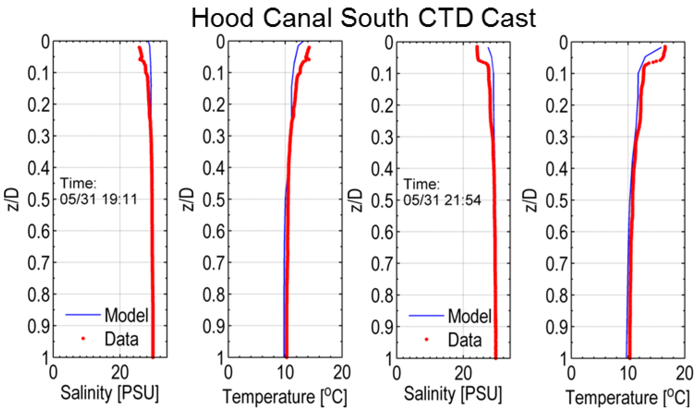
A series of CTD casts were also conducted north and south of the bridge. These CTD casts were collected at peak ebb and peak flood, as well as during slack water conditions. The observed salinity and temperature profiles were then compared with simulated temperature and salinity at the same location and time. Figure 8 and Figure 9 show examples of comparisons between observed and simulated salinity and temperature profiles at the north and south CTD cast locations, respectively.
The error statistics of temperature and salinity at the north and south CTD locations are also listed in Table 3. For temperature, both locations had AME ~0.5 °C with RMSE <0.8 °C. For salinity, AME and RMSE were 0.65 and 1.03 PSU, respectively. Although overall error statistics for the profiles were acceptable, examination of the results, especially for salinity, shows that the stratification in the upper 10% of the water column in the model is not as strong as in the data. This could be due to the limitation of the model confined to 10 sigma-layers. It could also be associated with near-field mixing induced by the bridge module as incorporated using the cell velocity block option. The results were similar for the three methods used for approximating the bridge block.
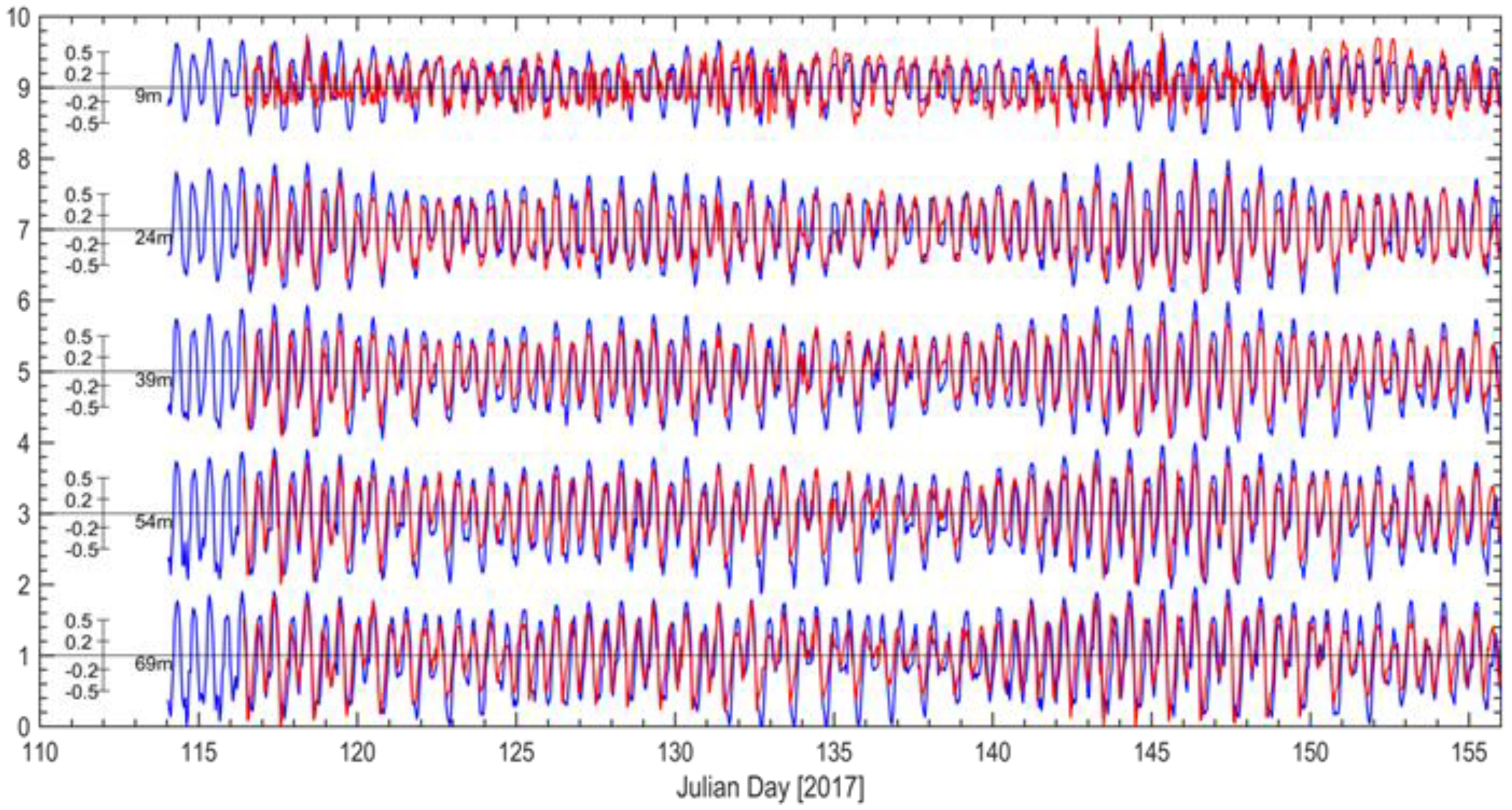
Currents: Current predictions at the North ADCP station, the South ADCP station, and the Bridge ADCP station were compared against field observations. The comparisons were selected at depths of 4 m, 9 m, 24 m, 39 m, 54 m, and 69 m. To better illustrate the comparison, velocities were decomposed into longitudinal and transversal components and are provided in Figure 10. The predicted phase of the velocity and the velocity magnitude associated with flooding and ebbing are in good agreement with the field observations. Figure 10 shows a comparison of predicted and observed velocities for different depths at the Bridge ADCP Station. At a depth of 9 m, the ADCP data bin nearest to the surface, the effect of HCB is reflected in both predicted and observed velocities.
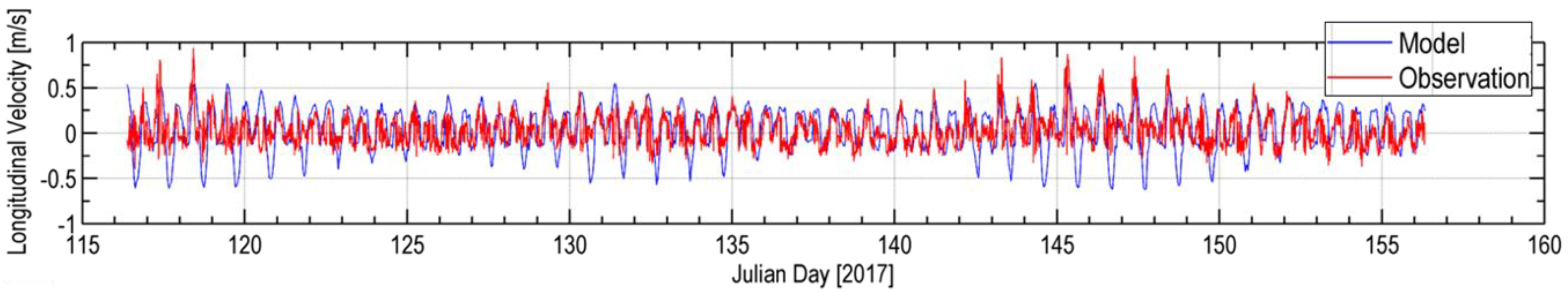
In addition to ADCP measurements, in an attempt to get as close to the bridge, pontoon, and hull as possible, a single-point measurement was conducted using an Aquadopp instrument, located 1 m below HCB. Figure 11 shows a comparison between predicted currents and observed data. The model appears to be overestimating the velocity during peak ebb. This region immediately below the bridge is known to generate eddies and shed vortices as the ebbing water is forced under the bridge. The model is unable to resolve these fine-scale eddies, which is one explanation for the error. Due to the fact that the model currently does not include skin friction at the bridge, the slip velocity in the model immediately below the bridge is, therefore, higher than the data.
The corresponding error statistics for current comparisons are summarized in Table 4. All stations had AME <0.03 m/s. The RMSE for all stations was <0.21 m/s, except for the Aquadopp single-point measurement, where a higher RMSE of 0.33 m/s was noted. It is noted that these errors are of magnitude comparable to the sustained swimming velocity of a 120-mm Juvenile Coho Salmon (~0.64 m/s) and the maximum swimming velocity for a 60–63-mm Juvenile Chum Salmon (~0.14 m/s) [22,23]. The WSS for the Aquadropp station was low (0.36) compared to other stations due to the complexity of the measurement. However, the WSS for the North ADCP, the South ADCP, and the Bridge ADCP was >0.89, suggesting that the model calibration results were of sufficient quality for use in ZOI calculations.
To assess the effect of HCB on near-field currents, we examined the data during peak ebb and flood periods for every tidal cycle at the North, South, and Bridge ADCP stations. The expectation was that the effect of the bridge on currents would be at a maximum during peak currents. Figure 12a shows the time series of depth-averaged longitudinal velocity at the bridge. Red triangles and yellow triangles indicate selected peak ebb and flood times, respectively, at which velocity information was extracted in each tidal cycle. The averages of predicted peak velocity profiles during flood and ebb are shown in Figure 12b–g along with measured data.
Positive velocity represents ebb or outflowing current direction due north toward the mouth of Hood Canal. Negative velocity indicates flood tidal currents due south in the opposite direction. Figure 12b–g show that the model is able to match the peak observed average velocity well at all stations during ebb and flood. The velocity reduction due to HCB is reproduced well by the model, as shown in Figure 12c,f. This confirms that the implementation of the bridge module in the Salish Sea model is successful in reproducing the reduction in velocity near the bridge. Small discrepancies were found at all stations that were attributed to approximations associated with smoothing of bathymetry and grid resolution. Similarly, representation of HCB in a sigma-coordinate framework required flattening of the depths immediately below the bridge, resulting in slightly higher velocities in the water column.
3. Results
3.1. Zone of Impact—Surface Layer
To characterize the bridge influence on the near-field environment, two sensitivity test scenario runs were performed. In test 1, the bridge block (1992 m long, 18.3 m wide, and 4.57 m deep) was completely removed, representing the conditions without the bridge. In test 2, the central (movable) span of the bridge with a length of 182 m was left in the open position with the bridge pontoons present in place. The central span is typically opened to allow ship and boat traffic to pass providing a third opening for tidal transport, with the two permanent openings present at the east and west ends of the bridge. To characterize the ZOI, baseline conditions from the summer of 2017 with the bridge in place were compared with the simulated results from the sensitivity tests (1) without the bridge and (2) with the central span open. Comparisons were conducted for predicted currents, salinity, and temperature, and ZOI estimates were obtained through quantifying the difference relative to existing or baseline conditions.
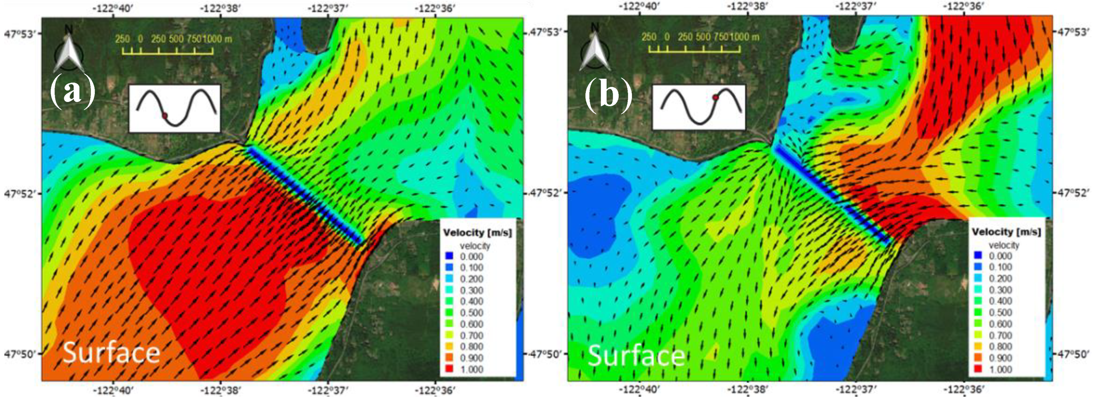
Figure 13 shows contour and velocity vector plots of existing conditions with HCB during ebb and flood. Peak ebb and flood times were selected during a typical spring tide on 27 April 2017, at 10:00 a.m. and 6:00 p.m., respectively, for this examination based on the expectation that maximum impact of the bridge block, reducing the currents to zero, would be strongest during the spring tides and during ebb and flood times. Figure 13a,b are currents with HCB present during the ebb and flood, respectively, for the surface layer. The surface layer occupies the upper 3% of the water column. The ebb currents in the surface layers are stronger than those during the flood. The effect of the HCB structure on currents is noticeable at the bridge where velocity was set to 0 m/s and a shadow of reduced currents exists immediately behind during both ebb and flood.
Figure 14 shows the same simulation but without the bridge with a much larger region occupied by currents in the >1 m/s bands.
Figure 15 shows surface layer currents with the central span open. The current patterns are similar to those at baseline conditions shown in Figure 13. Relative to the size (length) of the bridge blocking the surface layer, the central span represents an opening of ~9%. The effect of the opening on the currents is most visible in the form of the jet behind the bridge during both ebb and flood.
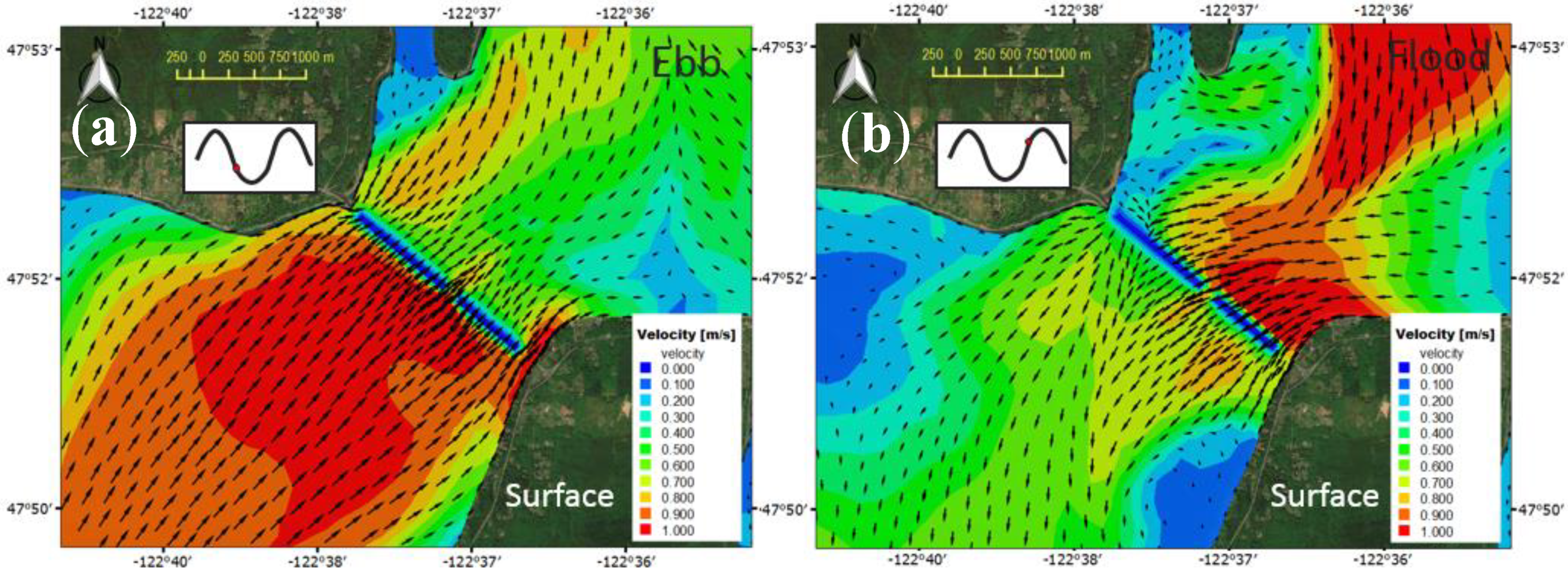
The ZOI is best characterized using plots of difference between simulated results from the baseline condition (with the bridge) relative to tests 1 and 2 to provide a direct assessment of the bridge impact. Figure 16a,b show a difference (reduction) in currents during peak ebb and flood with the bridge relative to test 1 without the bridge. Figure 16c,d show a reduction in currents during peak ebb and flood relative to the condition with the bridge draw span open. The effect of the bridge on surface currents is noticeable over a distance of ~1–2 Hood Canal widths in either direction (~2–5 km). Effect of the bridge span opening on currents is limited (~0.25 Hood Canal width, <600 m), but prominent during the ebb tide with stronger surface currents.
These difference plots in the plan view provide a qualitative estimate of the size of the ZOI for currents in the surface layer. The spatial pattern and extents were similar in nature with the influence of HCB most prominently seen behind the bridge during peak ebb and flood conditions. In all cases, the maximum difference of the baseline condition relative to the scenarios was at the bridge itself. In the surface layer, the maximum current difference was −0.88 m/s, the maximum salinity difference was +0.23 PSU, and the maximum temperature difference was −0.49 °C for the selected spring tide on 27 April 2017. The effect of the bridge dissipates with distance from the structure. Unlike velocity, where the effect is directly the result of blocked currents, the influence on salinity and temperature is more complex due to the presence of strong stratification and the increased mixing of surface layers at the bridge. Vertical transects analyzed in the next section provide a better understanding of the influence of the bridge on salinity and temperature.
3.2. Zone of Impact—Vertical Transect
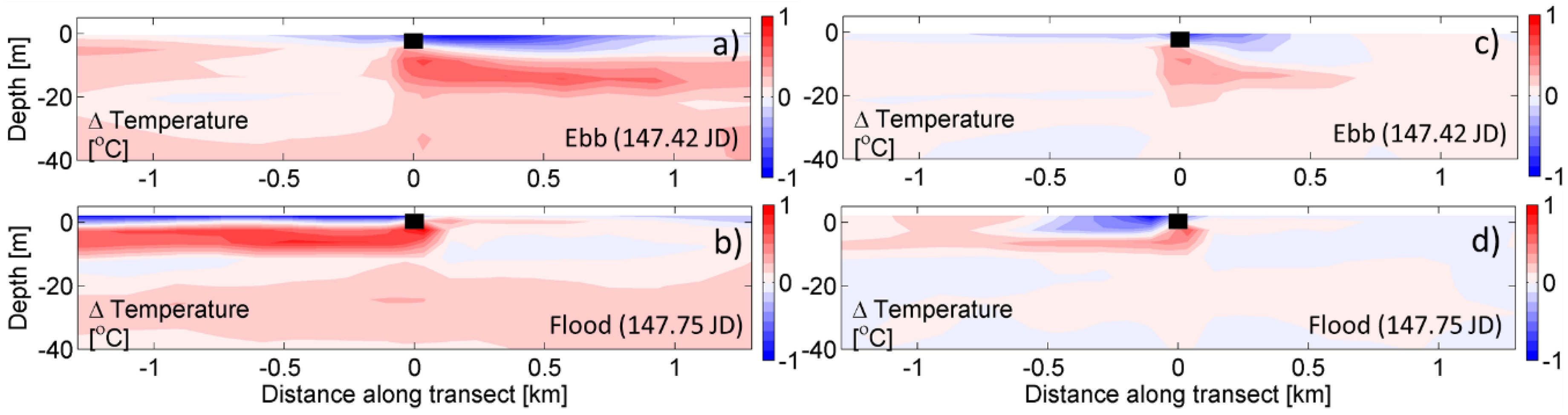
To further quantify the spatial extent of ZOI on current, salinity, and temperature variables in this environment with strong vertical stratification, simulation results were examined along a mid-channel transect across HCB. The assessment was done using two transects: (a) Transect-a, approximately 2.5 km long (length scale of Hood Canal width) across the bridge to provide a detailed characterization of near-field effects; and (b) Transect-b approximately 20 km long (distance from the bridge to the mouth of Hood Canal) to allow examination over larger distances over full tidal excursion (see Figure 17). The results were analyzed as difference plots similar to the plan view maps in the previous section, during the selected typical spring tide of 27 April 2017, at peak ebb (147.42 Julian days (JD), 27 May 2017 10:00 a.m.) and peak flood times (147.75 JD, 27 May 2017 6:00 p.m.).
The near-field effects of HCB on the current, salinity, and temperature in a vertical two-dimensional plane near the ZOI for the example spring tide period are shown in Figure 18, Figure 19 and Figure 20, respectively, using the shorter Transect-a. The distance between −1.25 km and 0 km represents the section south of the bridge, while that between 0 km and 1.25 km represents the downstream section north of the bridge. As in the surface plan view maps, a reduction in current magnitudes behind the bridge is seen during the flood and ebb. Figure 18a,b show that the currents are reduced behind the bridge relative to the scenario without the bridge. The vertical transect shows that the effect extends beyond the 1.25-km transect length on either side of the bridge and the effect is noticeable mostly in the upper ~10–15 m of the water column. Figure 18c,d show a similar relative difference in currents relative to the scenario with bridge draw span open. The effect is minor with a change of up to 0.3 m/s seen at the draw span opening, extending <500 m from the bridge.
Figure 19a,b show the effects of HCB on salinity through difference plots relative to test 1 without the bridge, during ebb and flood, respectively. The surface layer salinity immediately behind the bridge was higher. This was due to the blocking effect of the bridge holding the fresher (lower salinity) water back during flood and ebb. The traversing surface layer was forced to flow under the bridge, resulting in reduced salinity in the deeper layers below the bridge. A similar effect is seen relative to test 2 with the draw span open. Figure 19c,d show a small increase in surface salinity behind the bridge relative to the scenario with the draw span open. Plan view plots are consistent with velocity difference plots in that the effect of test 2 was restricted to a small region near the span opening. Salinity was lower in the layers immediately below the bridge due to fresher water being forced to lower layers by the presence of the bridge relative to the condition with draw span open.
The effect of HCB on temperature is similar to that predicted on salinity. Thermal stratification surface heat flux results in water temperatures in the surface layers being warmer than lower layers. The presence of the bridge holds the surface layers back, resulting in cooler waters immediately behind it relative to test 1 without the bridge during ebb and flood, as shown in Figure 20a,b. The warmer water was forced to traverse underneath the bridge, resulting in warmer waters in the deeper layers behind the bridge. Figure 20c,d show a similar effect but on a smaller scale with a small increase in surface temperature behind the bridge relative to the scenario with the draw span open. Temperatures were higher in the layers immediately below the bridge due to warmer water being forced to lower layers by the presence of the bridge relative to the condition with draw span open.
4. Discussion
Zone of Influence—Quantitative Assessment
The ZOI extends beyond the Hood Canal width scale of 2.4 km based on the results presented in Section 3. However, to quantify spatial extent, environmentally significant influence must first be defined. Maximum difference induced by HCB relative to test 1 on currents without the bridge occurred at the bridge itself and decayed or dissipated with distance from the bridge. For the purpose of this assessment, we defined ZOI as the distance at which the maximum difference (Δ) dropped to 10% of its value for current and salinity parameters (e.g., if maximum Δ = 1 m/s, then ZOI is where Δ = 0.1 m/s).
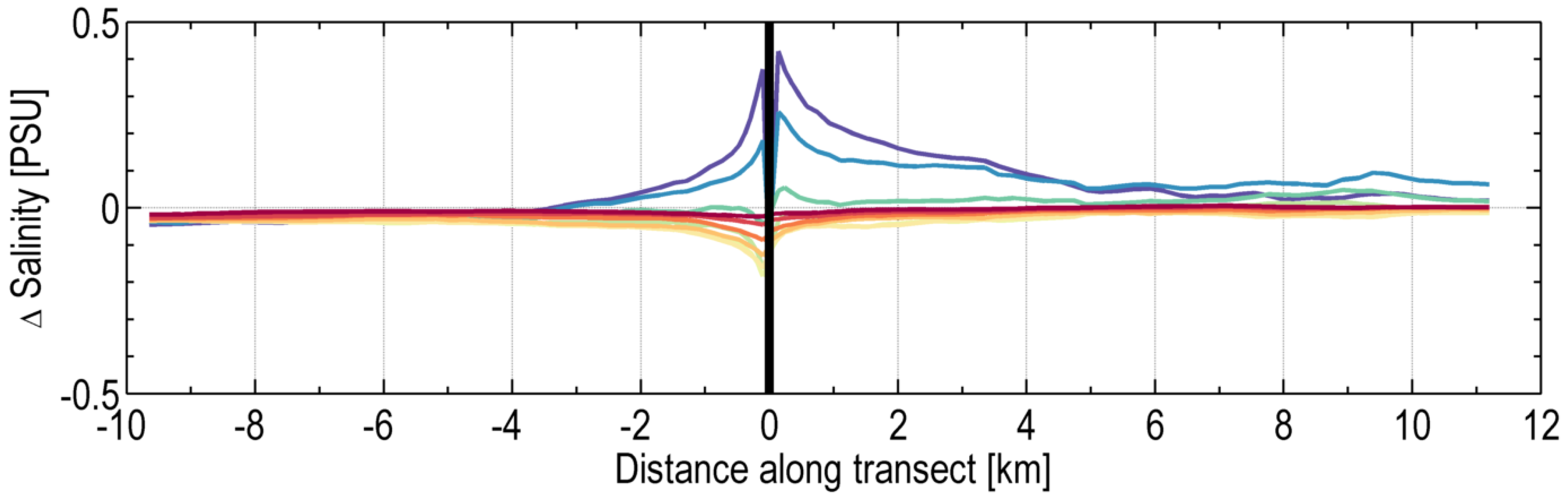
We first assessed the horizontal extent of ZOI by examining the changes in surface currents induced by the bridge relative to test 1. With a focus on impacts during peak tidal currents, we averaged multiple (71) peak ebb and peak flood instances over the calibration simulation period (25 April–11 June 2017). We then examined the vertical longitudinal extent of the ZOI by examining the relative difference of the variables for all depth layers along Transect-b over a distance of 20 km. Figure 21 shows the average difference in peak currents due to the presence of HCB relative to test 1 for the 10 model layers. The distance between −10 km and 0 km represents the region south of the bridge, while that between 0 km and 10 km represents the region north of the bridge. Model layers were distributed using a power law with an exponent of 1.5 such that layers had a higher concentration near the surface. Surface layer 1 occupied 3% of the water column and the bottom layer 10 occupied 15% of the water column. For currents, based on averaging multiple peak ebb and peak flood instances, maximum difference (−0.70 m/s) occurred during the ebb and in the surface layer, extending ~2.02 km north before dropping to −0.07 m/s (10% of the maximum difference). The maximum difference during the flood (−0.57 m/s) also occurred in the surface layer and the influence extended up to 3.43 km. It is interesting to note that, while there was a reduction in surface currents, the model generated a compensating increase in bottom-layer currents during flood, as well as ebb. The zone of influence, therefore, extends over the entire water column. It is important to note that this ZOI for currents is based on average impacts during peak currents. The ZOI spatial extent is smaller at all other times with smaller-magnitude currents.
Further examination of the results showed that, unlike velocity, peak instantaneous difference between baseline with bridge and test 1 without the bridge for temperature and salinity did not always occur at the bridge and occurred at various times in the tidal cycle. Peak instantaneous differences that vary in space and time make it difficult to define the ZOI. The approach for temperature and salinity was, therefore, to develop an average ZOI, taking into consideration all time steps.
Figure 22 shows the difference in salinity due to the presence of HCB relative to test 1 computed by averaging the differences over all hourly time steps for each layer. The average salinity difference results show a consistent pattern north and south of the bridge. The peak influence in average salinity occurred at the bridge, and, as described in Section 3, it was controlled by the mixing induced by the structure during ebb and flood. This resulted in an increase in salinity in the upper layers above the bridge draft depth (0–4.57 m) and a corresponding reduction in salinity in the lower layers below the draft from 4.57 m to ~20 m. The near-bed layers were unaffected. Also noticeable is the extent of the effect north of the bridge in the surface where the surface layers show elevated salinity levels ~+0.1 PSU that extend all the way to the mouth of Hood Canal. The effects of bridge-induced mixing resulted in higher salinity concentrations in the surface layers that were transported north in the surface outflow direction. This resulted in persistent and elevated levels of background salinity difference north of the bridge of 0.06 PSU over 4–10 km. The maximum difference (Δ) in salinity at the bridge was +0.42 PSU that extended 1.96 km to the south before dropping to 10% (0.04 PSU). ZOI determination to the north was complex as background salinity increased past the salinity 10% Δ level. The ZOI to the north was, therefore, provided as a range from 3.80 km where salinity Δ dropped to 10% above the background level of 0.1 PSU to Hood Canal mouth at ~10 km.
Figure 23 shows the difference in temperature due to the presence of the bridge relative to test 1 for the 10 model layers. The effect of HCB on temperature, based on averaging the difference for all hourly time steps over the period of 25 April–11 June 2017, was similar to that for salinity. The influence of the bridge on near-field temperature, due to the mixing induced by the bridge, resulted in a decrease in upper layer temperatures and an increase in temperature in lower layers below the draft from 4.57 m to ~20 m. The near-bed layers were unaffected. The effect of the bridge on temperature is noticeable in the downstream region north of the bridge where the surface layers showed a reduction in temperature levels that extended all the way to the mouth of Hood Canal. The maximum average difference (−0.49 °C) in the surface layers, a reduction in surface temperatures, dissipated to 10% ΔT (0.05 °C) ~2.23 km to the south. However, as in the case of salinity, temperature ZOI determination to the north was complex as there was a decrease in background temperature difference of 0.11 °C, over 4–10 km, that exceeded the temperature 10% ΔT level. The ZOI to the north was, therefore, provided as a range from 4.51 km where temperature ΔT dropped to 0.16 °C, 10% Δ above the background level, to Hood Canal mouth at ~10 km. It is noted, however, that the bridge caused an increase in temperatures in the lower layers of up to 0.20 °C.
Table 5 summarizes the ZOI dimensions for the parameters of interest examined using the criterion of a reduction in maximum difference Δ to 10% of its value.
Although the ZOI calculations and the values presented in Table 5 above used average values of maximum differences, it is noted that instantaneous differences could be as high as 1.22 m/s, 1.66 PSU, and 2.16 °C for velocity, salinity, and temperature, respectively.
5. Conclusions
A combination of oceanographic field data measurements and modeling-based assessment were used to ascertain whether the presence of HCB impacts near-field oceanographic parameters. While some effect was expected simply due to the existence of a large floating object in the path of the tidally influenced fjord-like waterbody of Hood Canal, the extent of influence was not quantified in the past. The results were conclusive in that both field data and model results showed that HCB blocks the movement of surface layer currents over ~85% of the width of Hood Canal. The openings at each end of the bridge (15% of the Hood Canal width) do carry a portion of the tidal flow; however, these openings are in shallow depths and do not fully compensate for the surface layer blockage. As a result, the current profile structure in the water column is altered. The reduction in surface layer currents and tidal flow is compensated by a corresponding increase in bottom-layer currents and flow. The impact is also felt in salinity and temperature magnitudes, particularly in the upper 20 m of the water column.
The ZOI was defined as the distances over which the difference in predicted maximum difference due to the presence of the bridge relative to the conditions without the bridge was reduced to 10% of its value. Based on the simulation conducted using 2017 spring conditions, the ZOI for current extends 3.43 km to the north and 2.02 km to the south of HCB. Maximum current difference based on the average of peak currents was −0.70 m/s at the surface layer. Similarly, the ZOI for salinity extends 3.80 km to the north and 1.96 km to the south, over which salinity deviated from the condition without the bridge. Maximum salinity difference was an increase of 0.42 PSU in the surface layers and an increase of 0.26 PSU in layers immediately below the bridge, based on a temporal average over the duration of the simulation. The ZOI for temperature extends 2.23 km to the south of HCB, over which temperature deviated from the condition without the bridge. Maximum temperature difference at the bridge was a decrease 0.49 °C in the surface layers and a decrease in temperature of 0.36 °C in layers immediately below the bridge, based on a temporal average over the duration of the simulation.
The near-field influence of the bridge on physical parameters of currents, salinity, and temperature as quantified by ZOI extends over 1.96 km to 5.15 km, which is roughly one to two Hood Canal width scales. Our study concludes that the influence on temperature and salinity is restricted to the upper 20 m, but extends through the water depth for current. The influence on temperature and salinity persists beyond the ZOI all the way to the mouth of Hood Canal at the confluence with Admiralty Inlet. The downstream effect is associated with fjord-like estuarine circulation. The brackish outflow in Hood Canal is restricted to surface layers. The presence of the bridge affects this net outflow through blockage and added turbulence and mixing. The persistent impact is seen in salinity and temperature downstream of the bridge, even after tides are averaged out.
Author Contributions
T.K. led the investigation and was responsible for conceptualization, methodology, and model development and application. T.W. developed the bridge module software. A.N. was responsible for processing and analysis of model results and field data. T.K. and A.N. analyzed the simulation results and developed the methodology for quantifying and summarizing the results.
Funding
This research was managed by Long Live the Kings through grants from the State of Washington. Funding was provided by Washington State with equal in-kind contributions by those participating in the research.
Acknowledgments
This publication is part of the Hood Canal Bridge Ecosystem Impact Assessment: an ecosystem-wide assessment of potential impacts of the Hood Canal Bridge on fish passage and water quality in Hood Canal.
Conflicts of Interest
The authors declare no conflict of interest. The funders had no role in the design of the study; in the collection, analyses, or interpretation of data; in the writing of the manuscript, and in the decision to publish the results.
References
- Puget Sound Partnership. 2009 State of the Sound Report; No. PSP09-08; Puget Sound Partnership: Olympia, WA, USA, 2010. [Google Scholar]
- Khangaonkar, T.; Yang, Z.; Kim, T.; Roberts, M. Tidally Averaged Circulation in Puget Sound Sub-basins: Comparison of Historical Data, Analytical Model, and Numerical Model. J. Estuar. Coast. Shelf Sci. 2011, 93, 305–319. [Google Scholar] [CrossRef]
- Khangaonkar, T.; Sackmann, B.; Long, W.; Mohamedali, T.; Roberts, M. Simulation of annual biogeochemical cycles of nutrient balance, phytoplankton bloom(s), and DO in Puget Sound using an unstructured grid model. Ocean Dyn. 2012, 62, 1353–1379. [Google Scholar] [CrossRef] [Green Version]
- Khangaonkar, T.; Nugraha, A.; Xu, W.; Long, W.; Bianucci, L.; Ahmed, A.; Mohamedali, T.; Pelletier, G. Analysis of Hypoxia and Sensitivity to Nutrient Pollution in Salish Sea. J. Geophys. Res. Oceans 2018, 123, 4735–4761. [Google Scholar] [CrossRef]
- Newton, J.; Bassin, C.; Devol, A.; Richey, J.; Kawase, M.; Warner, M. Chapter 1: Overview and Results Synthesis. In Integrated Assessment and Modeling Report; Hood Canal Dissolved Oxygen Program; University of Washington: Washington, DC, USA, 2011; Available online: http://www.hoodcanal.washington.edu/documents/document.jsp?id=3019 (accessed on 10 December 2018).
- Cope, B.; Roberts, M. Review and Synthesis of Available Information to Estimate Human Impacts to Dissolved Oxygen in Hood Canal; Ecology Publication No. 13-03-016; EPA Publication No. 910-R-13-002; Washington State Department of Ecology and U.S. EPA: Washington, DC, USA, 2013. Available online: https://fortress.wa.gov/ecy/publications/documents/1303016.pdf (accessed on 10 December 2018).
- Khangaonkar, T.; Wang, T. Potential alteration of fjordal circulation due to a large floating structure—Numerical investigation with application to Hood Canal basin in Puget Sound. Appl. Ocean Res. 2013, 39, 146–157. [Google Scholar] [CrossRef]
- Moore, M.; Berejikian, B.A.; Tezak, E.P. A floating bridge disrupts seaward migration and increases mortality of steelhead smolts in Hood Canal, Washington State. PLoS ONE 2013, 8, e73427. [Google Scholar] [CrossRef] [PubMed]
- Hood Canal Bridge Assessment Team. Hood Canal Bridge Ecosystem Impact Assessment Plan: Framework and Phase 1 Details; Long Live the Kings: Seattle, WA, USA, 2016; Available online: https://lltk.org/wp-content/uploads/2016/08/Hood-Canal-Bridge-Impact-Assessment-Plan-FINAL-27September2016.pdf (accessed on 10 December 2018).
- RPS. Current Measurements in Hood Canal Data Report; Maya Whitmont and Kevin Redmond of RPS Group PLC: Seattle, WA, USA, 2017. [Google Scholar]
- Chen, C.; Liu, H.; Beardsley, R.C. An unstructured, finite-volume, three-dimensional, primitive equation ocean model: Application Tocoastal Ocean and estuaries. J. Atmos. Ocean. Technol. 2003, 20, 159–186. [Google Scholar] [CrossRef]
- Cerco, C.; Cole, T. Three-Dimensional Eutrophication Model of Chesapeake Bay; Tech. Rep. EL-94-4; U.S. Army Corps of Engineers: Vicksburg, MI, USA, 1994. [Google Scholar]
- Cerco, C.F.; Cole, T.M. User’s Guide to the CE-QUAL-ICM Three-Dimensional Eutrophication Model; Release Version 1.0; U.S. Army Corps of Engineers: Washington, DC, USA, 1995; p. 320. [Google Scholar]
- Khangaonkar, T.; Long, W.; Xu, W. Assessment of circulation and inter-basin transport in the Salish Sea including Johnstone Strait and Discovery Islands pathways. Ocean Model. 2017, 109, 11–32. [Google Scholar] [CrossRef]
- Bianucci, L.; Long, W.; Khangaonkar, T.; Pelletier, G.; Ahmed, A.; Mohamedali, T.; Roberts, M.; Figueroa-Kaminsky, C. Sensitivity of the regional ocean acidification and the carbonate system in Puget Sound to ocean and freshwater inputs. Elem. Sci. Anthropocene 2018, 6, 22. [Google Scholar] [CrossRef]
- Mohamedali, T.; Roberts, M.; Sackmann, B.S.; Kolosseus, A. Puget Sound Dissolved Oxygen Model: Nutrient Load Summary for 1999–2008; Publication No. 11-03-057; Washington State Department of Ecology: Olympia, WA, USA, 2011. [Google Scholar]
- Spargo, E.; Westerink, J.; Luettich, R.; Mark, D. Developing a Tidal Constituent Database for the Eastern North Pacific Ocean. In Proceedings of the 8th International Conference on Coastal Modeling, Mexico City, Mexico, 18–24 February 2007. [Google Scholar]
- Locarnini, R.A.; Mishonov, A.V.; Antonov, J.I.; Boyer, T.P.; Garcia, H.E.; Baranova, O.K.; Zweng, M.M.; Paver, C.R.; Reagan, J.R.; Johnson, D.R.; et al. World Ocean Atlas 2013; Volume 1: Temperature; NOAA Atlas NESDIS 73; Levitus, S., Mishonov, A., Eds.; National Oceanic and Atmospheric Administration: Silver Spring, MD, USA, 2013; p. 40. [Google Scholar]
- Zweng, M.M.; Reagan, J.R.; Antonov, J.I.; Locarnini, R.A.; Mishonov, A.V.; Boyer, T.P.; Garcia, H.E.; Baranova, O.K.; Johnson, D.R.; Seidov, D.; et al. World Ocean Atlas 2013; Volume 2: Salinity; NOAA Atlas NESDIS 74; Lev-itus, S., Mishonov, A., Eds.; National Oceanic and Atmospheric Administration: Silver Spring, MD, USA, 2013; p. 39. [Google Scholar]
- Willmott, C.J. Some comments on the evaluation of model performance. Bull. Am. Meteorol. Soc. 1982, 63, 1309–1313. [Google Scholar] [CrossRef]
- Wang, T.; Khangaonkar, T.; Long, W.; Gill, G. Development of a Kelp-Type Structure Module in a Coastal Ocean Model to Assess the Hydrodynamic Impact of Seawater Uranium Extraction Technology. J. Mar. Sci. Eng. 2014, 2, 81–92. [Google Scholar] [CrossRef]
- Wissmar, R.; Simenstad, C. Energetic Constraints of Juvenile Chum Salmon (Oncorhynchus keta) Migrating in Estuaries. Can. J. Fish. Aquat. Sci. 1988, 45, 1555–1560. [Google Scholar] [CrossRef]
- Greene, C.M.; Hall, J.; Small, D.; Smith, P. Effects of Intertidal Water Crossing Structures on Estuarine Fish and Their Habitat: A Literature Review and Synthesis. 2017. Available online: http://www.skagitclimatescience.org/wp-content/uploads/2018/07/Greene-et-al.-2017-review-on-intertidal-water-crossing-structures-and-fish-1.pdf (accessed on 10 December 2018).
Figure 1.
(a) Oceanographic regions of Salish Sea including Northwest Straits, Puget Sound, and the inner sub-basins—Hood Canal, Whidbey Basin, Central Basin, and South Sound; (b) bathymetric profile of Hood Canal study area.
Figure 1.
(a) Oceanographic regions of Salish Sea including Northwest Straits, Puget Sound, and the inner sub-basins—Hood Canal, Whidbey Basin, Central Basin, and South Sound; (b) bathymetric profile of Hood Canal study area.

Figure 2.
Hood Canal Bridge (HCB) study area showing the floating bridge and the 2017 oceanographic data collection program station locations relative to the bridge.
Figure 2.
Hood Canal Bridge (HCB) study area showing the floating bridge and the 2017 oceanographic data collection program station locations relative to the bridge.

Figure 3.
(a) Salish Sea model domain and finite-volume grid; (b) monthly water-quality monitoring stations from Washington State Department of Ecology.
Figure 3.
(a) Salish Sea model domain and finite-volume grid; (b) monthly water-quality monitoring stations from Washington State Department of Ecology.

Figure 4.
HCB layout with pontoon cross-section and east span details. Detail A is a sectional view across the width of the bridge.
Figure 4.
HCB layout with pontoon cross-section and east span details. Detail A is a sectional view across the width of the bridge.

Figure 5.
Salish Sea model grid with refinement in the region to facilitate incorporation of the bridge block elements. The grid size is refined such that cell centers are separated by the bridge width distance of 18.3 m. The bridge draft is represented by two layers whose combined thickness is equal to 4.57 m.

Figure 6.
Time series of model result, NOAA harmonic (Xtide) prediction, and observed data for sea-water elevation. Time is shown as Julian days in 2017.
Figure 6.
Time series of model result, NOAA harmonic (Xtide) prediction, and observed data for sea-water elevation. Time is shown as Julian days in 2017.

Figure 7.
Time series of model results and observed data for salinity (left panel) and temperature (right panel) from 31 May and 1 June 2017. Plots (a,d) are a comparison for the North acoustic Doppler current profiler (ADCP) station; plots (b,e) are for the Bridge ADCP station; and plots (c,f) are for the South ADCP station.

Figure 8.
Comparisons of predicted and observed salinities at peak ebb and peak flood north of HCB on 31 May 2017.
Figure 8.
Comparisons of predicted and observed salinities at peak ebb and peak flood north of HCB on 31 May 2017.

Figure 9.
Comparisons of predicted and observed salinities at peak ebb and peak flood south of HCB on 31 May 2017.
Figure 9.
Comparisons of predicted and observed salinities at peak ebb and peak flood south of HCB on 31 May 2017.

Figure 10.
Comparisons of predicted (blue) and observed (red) velocities for different depths at the Bridge ADCP station (example).
Figure 10.
Comparisons of predicted (blue) and observed (red) velocities for different depths at the Bridge ADCP station (example).

Figure 11.
Comparisons of predicted and observed velocities just below HCB.

Figure 12.
(a) Time series of depth-averaged velocity at bridge; (b–g) comparisons of predicted and observed average velocity profiles at the South, Bridge, and North ADCP stations during maximum flood and ebb tide periods. Gray thin lines represent daily velocity profiles during peak ebb and flood periods.

Figure 13.
Predicted horizontal velocity contour and vector plots for the baseline scenario with HCB present for (a) ebb and (b) flood currents in the surface layer. (Typical spring tide on 27 April 2017).
Figure 13.
Predicted horizontal velocity contour and vector plots for the baseline scenario with HCB present for (a) ebb and (b) flood currents in the surface layer. (Typical spring tide on 27 April 2017).

Figure 14.
Predicted horizontal velocity contour and vector plots for test 1 scenario without HCB present for (a) ebb and (b) flood currents in the surface layer. (Typical spring tide on 27 April 2017).
Figure 14.
Predicted horizontal velocity contour and vector plots for test 1 scenario without HCB present for (a) ebb and (b) flood currents in the surface layer. (Typical spring tide on 27 April 2017).

Figure 15.
Predicted horizontal velocity contour and vector plots for test 2 scenario with HCB present and middle span open for (a) ebb and (b) flood currents in the surface layer. (Typical spring tide on 27 April 2017).
Figure 15.
Predicted horizontal velocity contour and vector plots for test 2 scenario with HCB present and middle span open for (a) ebb and (b) flood currents in the surface layer. (Typical spring tide on 27 April 2017).

Figure 16.
(a,b) Velocity difference of baseline scenario with HCB relative to test 1 without HCB during peak ebb and flood; (c,d) velocity difference of baseline scenario with HCB relative to test 2 with draw span open during ebb and flood. (Typical spring tide on 27 April 2017).
Figure 16.
(a,b) Velocity difference of baseline scenario with HCB relative to test 1 without HCB during peak ebb and flood; (c,d) velocity difference of baseline scenario with HCB relative to test 2 with draw span open during ebb and flood. (Typical spring tide on 27 April 2017).

Figure 17.
Transects for assessment of zone of influence (ZOI) in a vertical plane: (a) short transect for near-field effects; (b) longer transect to examine the effects over full tidal excursion.
Figure 17.
Transects for assessment of zone of influence (ZOI) in a vertical plane: (a) short transect for near-field effects; (b) longer transect to examine the effects over full tidal excursion.

Figure 18.
(a,b) Velocity difference of baseline scenario with HCB relative to test 1 without HCB during peak ebb and flood; (c,d) velocity difference of baseline scenario with HCB relative to test 2 with draw span open during ebb and flood. (Typical spring tide on 27 April 2017).
Figure 18.
(a,b) Velocity difference of baseline scenario with HCB relative to test 1 without HCB during peak ebb and flood; (c,d) velocity difference of baseline scenario with HCB relative to test 2 with draw span open during ebb and flood. (Typical spring tide on 27 April 2017).

Figure 19.
(a,b) Salinity difference of baseline scenario with HCB relative to test 1 without HCB during peak ebb and flood; (c,d) velocity difference of baseline scenario with HCB relative to test 2 with draw span open during ebb and flood. (Typical spring tide on 27 April 2017).
Figure 19.
(a,b) Salinity difference of baseline scenario with HCB relative to test 1 without HCB during peak ebb and flood; (c,d) velocity difference of baseline scenario with HCB relative to test 2 with draw span open during ebb and flood. (Typical spring tide on 27 April 2017).

Figure 20.
(a,b) Temperature difference of baseline scenario with HCB relative to test 1 without HCB during peak ebb and flood; (c,d) velocity difference of baseline scenario with HCB relative to test 2 with draw span open during ebb and flood. (Typical spring tide on 27 April 2017).
Figure 20.
(a,b) Temperature difference of baseline scenario with HCB relative to test 1 without HCB during peak ebb and flood; (c,d) velocity difference of baseline scenario with HCB relative to test 2 with draw span open during ebb and flood. (Typical spring tide on 27 April 2017).

Figure 21.
Difference in current magnitudes due to HCB relative to test 1, plotted along Transect-b for all model layers. The (top) panel presents peak ebb and the (bottom) panel presents peak flood results averaged over the calibration period of 25 April–11 June 2017. (The distance between −10 km and 0 km represents the region south of the bridge, while that between 0 km and 10 km represents the region north of the bridge).

Figure 22.
Difference in salinity due to HCB relative to test 1, plotted along Transect-b for all model layers. The plot shows average salinity difference for all hourly time steps over the calibration period of 25 April–11 June 2017. (The distance between −10 km and 0 km represents the region south of the bridge, while that between 0 km and 10 km represents the region north of the bridge).

Figure 23.
Difference in temperature due to HCB relative to test 1, plotted along Transect-b for all model layers. The plot shows average temperature difference for all hourly time steps over the calibration period of 25 April–11 June 2017. (The distance between −10 km and 0 km represents the region south of the bridge, while that between 0 km and 10 km represents the region north of the bridge).


Table 1.
Salish Sea model overall error statistics and skill score for temperature and salinity calibration data for the year 2014 from monthly monitoring profiles.
Table 1.
Salish Sea model overall error statistics and skill score for temperature and salinity calibration data for the year 2014 from monthly monitoring profiles.
| Mean Error (Bias) | RMSE | WSS | |||||||
|---|---|---|---|---|---|---|---|---|---|
| Max | Min | Ave | Max | Min | Ave | Max | Min | Ave | |
| T (°C) | 0.97 | −1.77 | −0.03 | 2.29 | 0.40 | 0.94 | 0.99 | 0.78 | 0.94 |
| S (PSU) | 0.09 | −0.93 | −0.24 | 2.27 | 0.39 | 0.96 | 0.90 | 0.60 | 0.80 |
RMSE = root-mean-square error; WSS = Willmott skill score; T = temperature; S = salinity; PSU = practical salinity unit; Max = maximum value of site-specific error statistic among 21 Puget Sound stations; Min = minimum value of site-specific error statistic among 21 Puget Sound stations; Ave = global error statistic considering data and model results from all stations.
Table 2.
Salish Sea model calibration error statistics and skill score for water elevation. AME = absolute mean error.
Table 2.
Salish Sea model calibration error statistics and skill score for water elevation. AME = absolute mean error.
| AME | RMSE | WSS | |
|---|---|---|---|
| Elevation (m) | 0.013 | 0.420 | 0.960 |
Table 3.
Salish Sea model validation error statistics and skill score for temperature and salinity at different locations near Hood Canal Bridge (HCB). ADCP = acoustic Doppler current profiler; CTD = conductivity, temperature, and depth.
Table 3.
Salish Sea model validation error statistics and skill score for temperature and salinity at different locations near Hood Canal Bridge (HCB). ADCP = acoustic Doppler current profiler; CTD = conductivity, temperature, and depth.
| Station | Temperature | Salinity | ||||
|---|---|---|---|---|---|---|
| AME | RMSE | WSS | AME | RMSE | WSS | |
| North ADCP | 0.22 | 0.56 | 0.74 | 0.21 | 0.57 | 0.30 |
| South ADCP | 0.08 | 0.40 | 0.85 | 0.12 | 0.36 | 0.41 |
| Bridge ADCP | 0.41 | 0.79 | 0.90 | 0.82 | 1.29 | 0.47 |
| North CTD | 0.47 | 0.91 | 0.80 | 0.33 | 0.86 | 0.68 |
| South CTD | 0.50 | 0.80 | 0.90 | 0.65 | 1.03 | 0.72 |
Table 4.
Salish Sea model calibration error statistics and skill score for velocities.
| Station | AME | RMSE | WSS |
|---|---|---|---|
| North ADCP | 0.00 | 0.14 | 0.94 |
| South ADCP | 0.02 | 0.21 | 0.89 |
| Bridge ADCP | 0.03 | 0.21 | 0.92 |
| Aquadopp | 0.02 | 0.33 | 0.36 |
Table 5.
Summary of zone of influence (ZOI) characterizing distances over which the difference in predicted maximum difference Δ due to the presence of the bridge relative to the test 1 scenario without the bridge was reduced to 10% of its value. Results in this table are based on an average of all peak ebb and flood instances over the period of 25 April–11 June 2017 for velocity, and an average of all time steps for salinity and temperature.
| Variable | Max. (Δ) | South HCB | North HCB |
|---|---|---|---|
| ZOI (km) | ZOI (km) | ||
| Velocity (m/s) | −0.70 | 2.02 | 3.43 |
| Salinity (PSU) | 0.42 | 1.96 | 3.80–10 |
| Temperature (°C) | −0.49 | 2.23 | 4.51–10 |
© 2018 by the authors. Licensee MDPI, Basel, Switzerland. This article is an open access article distributed under the terms and conditions of the Creative Commons Attribution (CC BY) license (http://creativecommons.org/licenses/by/4.0/).
Share and Cite
MDPI and ACS Style
Khangaonkar, T.; Nugraha, A.; Wang, T. Hydrodynamic Zone of Influence Due to a Floating Structure in a Fjordal Estuary—Hood Canal Bridge Impact Assessment. J. Mar. Sci. Eng. 2018, 6, 119. https://doi.org/10.3390/jmse6040119
AMA Style
Khangaonkar T, Nugraha A, Wang T. Hydrodynamic Zone of Influence Due to a Floating Structure in a Fjordal Estuary—Hood Canal Bridge Impact Assessment. Journal of Marine Science and Engineering. 2018; 6(4):119. https://doi.org/10.3390/jmse6040119
Chicago/Turabian StyleKhangaonkar, Tarang, Adi Nugraha, and Taiping Wang. 2018. "Hydrodynamic Zone of Influence Due to a Floating Structure in a Fjordal Estuary—Hood Canal Bridge Impact Assessment" Journal of Marine Science and Engineering 6, no. 4: 119. https://doi.org/10.3390/jmse6040119
Note that from the first issue of 2016, this journal uses article numbers instead of page numbers. See further details here.