Response-Spectrum Uncoupled Analyses for Seismic Assessment of Offshore Wind Turbines


Department of Civil, Energy, Environmental and Materials Engineering (DICEAM), University of Reggio Calabria, 89124 Reggio Calabria, Italy
*
Author to whom correspondence should be addressed.
J. Mar. Sci. Eng. 2018, 6(3), 85; https://doi.org/10.3390/jmse6030085
Submission received: 30 May 2018
/
Revised: 28 June 2018
/
Accepted: 29 June 2018
/
Published: 9 July 2018
(This article belongs to the Special Issue Offshore Wind Structures)
Abstract
:According to International Standards and Guidelines, the seismic assessment of offshore wind turbines in seismically-active areas may be performed by combining two uncoupled analyses under wind-wave and earthquake loads, respectively. Typically, the separate earthquake response is calculated by a response-spectrum approach and, for this purpose, structural models of various degrees of complexity may be used. Although response-spectrum uncoupled analyses are currently allowed as alternative to time-consuming fully-coupled simulations, for which dedicated software packages are required, to date no specific studies have been presented on whether accuracy may vary depending on key factors as structural modelling, criteria to calculate wind-wave and earthquake responses, and other relevant issues as the selected support structure, the considered environmental states and earthquake records. This paper will investigate different potential implementations of response-spectrum uncoupled analyses for offshore wind turbines, using various structural models and criteria to calculate the wind-wave and earthquake responses. The case study is a 5-MW wind turbine on two support structures in intermediate waters, under a variety of wind-wave states and real earthquake records. Numerical results show that response-spectrum uncoupled analyses may provide non-conservative results, for every structural model adopted and criteria to calculate wind-wave and earthquake responses. This is evidence that appropriate safety factors should be assumed when implementing response-spectrum uncoupled analyses allowed by International Standards and Guidelines.
1. Introduction
International Standards and Guidelines, such as IEC 61400-3 [1], GL 2012 [2] and DNV-OS-J101 [3], recommend a seismic assessment of offshore bottom-fixed horizontal-axis wind turbines (HAWTs) in seismically-active areas. Bottom-fixed HAWTs are typically installed in water depths from shallow (<30 m) to intermediate (30–60 m) ones and, in view of the fact that there exist several offshore sites at medium-to-high seismic risk, with high wind resources and water depth up to 60 m [4,5,6], efficiency and accuracy of methods for a seismic assessment have become of crucial interest. This is particularly true considering that, in general, offshore HAWTs may be more prone to seismic loads than land-based ones, as they feature taller support structures and larger-size turbines to exploit higher wind resources at sea.
Studies have investigated the seismic response of offshore HAWTs mounted on monopiles [7,8] or support structures including a jacket or a tripod [9]. A simplified model or a full system model has been used: The first involves the support structure only, with the rotor-nacelle assembly (RNA) modelled as a lumped mass at the tower top [7,8]; the second includes the support structure and whole turbine, i.e., rotor blades, nacelle, as well as mechanical/electrical/control turbine components [9]. Various scenarios for earthquake striking have been considered, with the rotor in a parked state [7,8,9] or operational conditions [9]. Specifically, Alati et al. [9] have run time-domain, fully-coupled simulations on full system models of the baseline 5-MW HAWT of the National Renewable Energy Laboratory (NREL) [10], mounted on a jacket or a tripod in intermediate waters, for a large set of earthquakes. A comprehensive review on seismic analysis of offshore HAWTs and related issues may be found in a recent paper by Katsanos et al. [11].
The reference numerical tool to calculate the response of offshore HAWTs under simultaneous wind, waves and earthquake ground motion is a time-domain, nonlinear fully-coupled simulation. Alternatively, International Standards and Guidelines allow uncoupled analyses, where the responses to wind-wave loads and earthquake loads are computed separately and linearly combined [1,2,3]. In the implementation of uncoupled analyses for offshore HAWTs, the separate wind-wave response is typically computed from a time-domain simulation, while the separate earthquake response may be computed in time domain [2] or by a response-spectrum approach [1,2,3], in agreement with similar prescriptions for land-based HAWTs [12,13,14]. The response-spectrum approach may appear particularly appealing, because it can readily be implemented in commercial finite-element (FE) software packages and involves concepts most structural engineers are familiar with. For the implementation of response-spectrum uncoupled analyses, International Standards and Guidelines allow structural models of different complexity and various criteria to calculate wind-wave and earthquake responses. DNV-OS-J101 [3] prescribe that, at least, three modes are included in the analysis and that corresponding modal responses are combined by a Complete Quadratic Combination (CQC) method [15]. In this context, when the earthquake response is combined with operational wind-wave loads, 5% damped response spectra are generally used. Considering that structural damping ratio amounts generally to 1% for typical steel support structures, this corresponds to assume a 4% aerodynamic damping when computing the separate earthquake response [14,16,17,18,19,20,21]. In addition, IEC 61400-3 [1] allows an approximate response-spectrum approach on a simplified model with a lumped mass at the top, where the separate earthquake response is computed from a 1% damped spectrum and combined with an emergency-shutdown wind-wave response at rated wind speed. This approach mirrors the approximate approach suggested by Annex C of IEC 61400-1 for land-based HAWTs [12].
While there exist studies on response-spectrum uncoupled analyses for land-based HAWTs, e.g., see ref. [22], to the best of authors’ knowledge no specific investigations have been carried out on the accuracy of response-spectrum uncoupled analyses for offshore HAWTs. Yet, assessing the accuracy against time-domain fully-coupled simulations is crucial, because coupling effects in the response of offshore HAWTs may be significant due to the interactions among aerodynamic-hydrodynamic-seismic responses. On the other hand, it is of great interest to check whether the accuracy may depend on the structural modelling, as well as the criteria to calculate wind-wave and earthquake responses. Other issues, depending on which the accuracy of uncoupled analyses may vary, are the support structure adopted as well as the considered environmental states and earthquake records.
Investigating the accuracy of response-spectrum uncoupled analyses for offshore HAWTs is the main objective of this paper. In particular, the baseline 5-MW NREL wind turbine [10] is considered, mounted on a jacket and a tripod in intermediate water depth. For each support structure, four structural models are built:
- Full Model: a multi-body model with support structure, rotating rotor as well as electrical/mechanical/control components.
- FE Model 1: a FE model including support structure and rotor in parked state.
- FE Model 2: a FE model including support structure and a lumped mass at the tower top = mass of the RNA.
- FE Model 3: a FE model of the support structure, with a lumped mass at the tower top including mass of the RNA and mass of the support-structure upper part lying above half of the total height; the support structure is considered as massless. The model is based on the prescriptions of Annex C of IEC 61400-1 [12].
The Full Model is implemented in GH-BLADED [23] while FE Models 1-2-3 are implemented in SAP 2000 [24]. The models are used in three methods of uncoupled analyses, Methods 1-2-3, which involve different criteria to calculate the maxima wind-wave and earthquake responses. Results will be compared with those from time-domain fully-coupled simulations on the Full Model, for various wind-wave states and real earthquake records with two horizontal components.
2. Test Structures
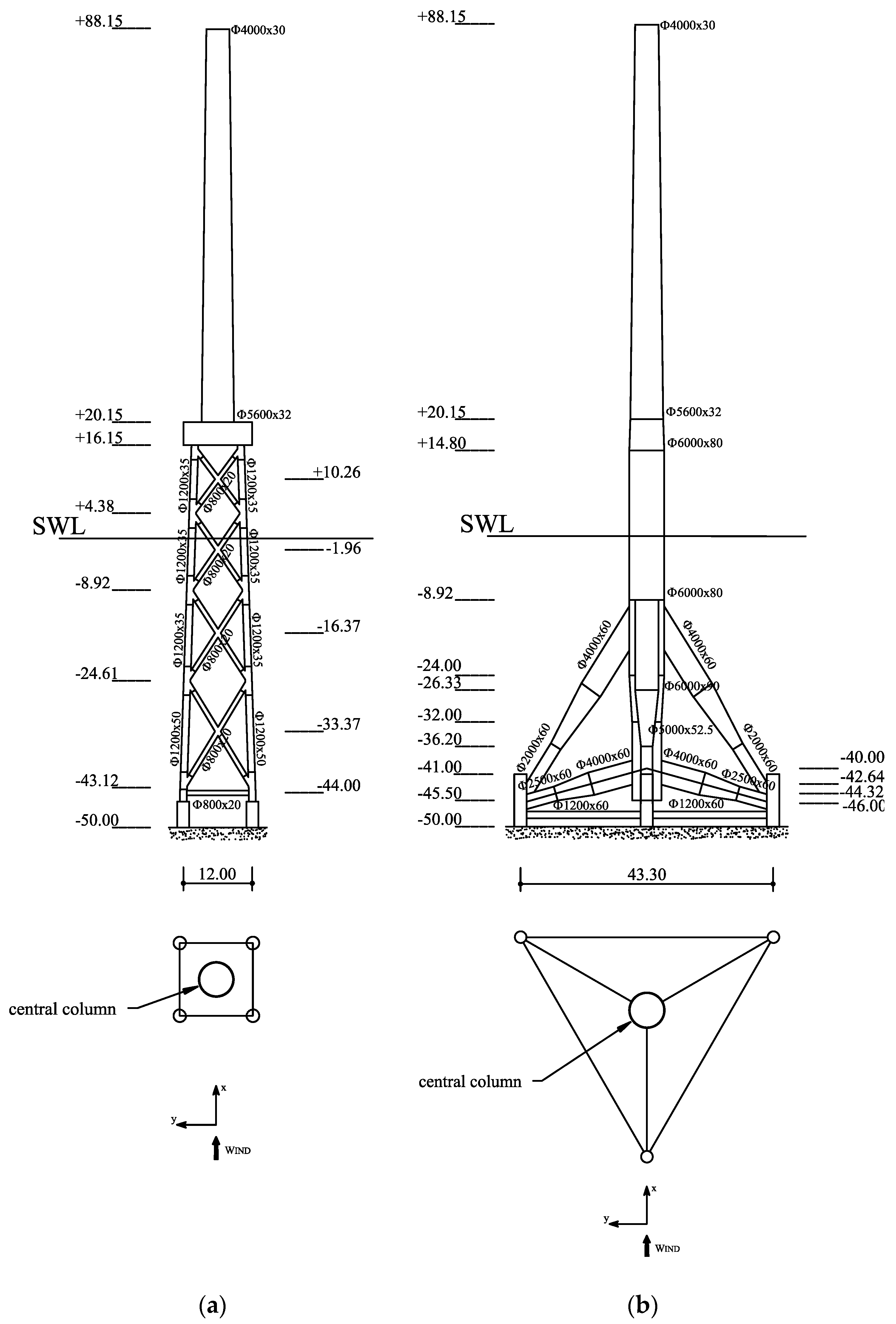
The turbine is the NREL 5-MW three-bladed HAWT [10], which is generally taken as representative of modern multi-megawatt wind turbines in recent literature [25,26,27,28,29,30]. Two steel support structures are considered, the centre-column jacket and tripod shown in Figure 1, designed according to current practice [9,31]. The jacket is a four-legged multimember structure, as typically used in offshore oil and gas industry, while the tripod is fabricated from three tubular members welded to a central one, and additional smaller members welded to each other; both are equipped with short tubing at the corners providing guides for pile foundations. Details on structural members are given in Figure 2. Steel parameters for the support structures are: Young’s modulus = 210 GPa, Poisson coefficient = 0.3, mass density = 7850 kg/m3. Rotor blades are made of glass-fiber composite material, with elastic properties at various stations along the blade provided in the reference dataset [10]. It is assumed that the water depth is 50 m. Insight into technological and design aspects of support structures at this water depth may be found in ref. [32,33].
In the following, the two test structures in Figure 1 will be referred to as “Jacket” and “Tripod”.
3. Structural Models
For the purposes of this study, a Full Model and three FE Models, FE Models 1-2-3, are constructed for both Jacket and Tripod in Figure 1, as detailed in the following:
- Full Model implemented in GH-BLADED [23], a software package validated by Germanischer-Lloyd for analysis and certification of offshore HAWTs. GH-BLADED adopts a multi-body approach combining FEs for flexible members with rigid bodies for mechanical components. Two-node shear-deformable Timoshenko beam elements are used for structural members of the support structure and blades with, in particular, a total number of 134 FEs and 67 FEs for the support structures of Jacket and Tripod, respectively; 49 FEs for each blade, with varying flapwise and edgewise flexural stiffness at the nodes set, according to the reference dataset [10]. Parameters in the reference dataset are also used to model nacelle, drive train, as well as mechanical/electrical/control components, for a full representation of wind turbine aerodynamics [10]. The multi-body approach of GH-BLADED includes nonlinearity arising from large displacements of the rotor with respect to the support structure.
- FE Model 1 implemented in SAP 2000 [24]: Support structure and rotor blades are modelled by two-node shear-deformable Timoshenko beam elements. The rotor is assumed to be in parked state, with one blade upward and two blades downward. A total number of 134 FEs and 67 FEs are used for modelling the support structures of Jacket and Tripod, respectively, i.e., exactly the same number used for the multi-body Full Model in GH-BLADED. Likewise, 49 FEs are used for each blade, again with varying flapwise and edgewise flexural stiffness at the nodes set according to the reference dataset [10], while the nacelle is modelled by 2 rigid FEs. The model is implemented based on the standard theory of small displacements.
- FE Model 2 implemented in SAP 2000: The support structure is modelled by two-node shear-deformable Timoshenko beam elements as in FE model 1, while the RNA is reverted to a lumped mass at the tower top, equal to 3.5 × 10⁵ kg, see reference [10]. Again, the standard theory of small displacements is considered.
- FE Model 3 implemented in SAP 2000, according to the prescriptions in Annex C of IEC 61400-1 [12]. It is a simplified two-degree-of-freedom system. The support structure is massless and modelled by shear-deformable Timoshenko beam elements, using again 134 FEs and 67 FEs for Jacket and Tripod respectively, as in FE Models 1-2 and Full Model. A lumped mass is placed at the top, including the mass of the RNA (= 3.5 × 10⁵ kg, see reference [10]) and the mass of the support-structure upper part lying above half of the total height, i.e., above 69 m from the seabed (69 = (88.15 + 50)/2), which is equal to 6.04 × 10⁵ kg in the Jacket and 2.53 × 10⁵ kg in the Tripod. Again, the standard theory of small displacements is considered.
All models are assumed to be clamped at the mudline (−50 m).
Table 1 reports the modal frequencies of the Full Model in GH-BLADED, considering the rotor in a parked state (one blade upward, two blades downward), along with those of FE Models 1-2 in SAP 2000. In GH-BLADED, modes are built combining uncoupled rotor and support-structure modes, using for this a specific linearization module coupling the equations of motion [23], while modes in SAP 2000 are built by a standard small-displacement modal analysis approach. Fore-aft and side-to-side directions correspond to x and y directions in Figure 1, respectively. Natural frequencies in Table 1 are in agreement with typical ones in the literature [31,34] and differences between Full Model in GH-BLADED and FE Models 1-2 in SAP 2000 are within engineering margins.
Table 2 reports the natural frequencies of FE Model 3 associated with the horizontal displacements of the tower top in fore-aft and side-to-side directions. They are computed based on top lumped mass and stiffness of FE Model 3, with stiffness obtained by applying at the tower top unit point forces in x and y directions, respectively (see Figure 1). Differences from those of the corresponding natural frequencies of Full Model in Table 1 (see 1st support-structure modes in fore-aft and side-to-side directions) are up to 26% and 14% for Jacket and Tripod. This means that reverting the whole mass of the system to a lumped mass at the top, as prescribed by Annex C of IEC 61400-1 [12], represents a rather approximate description of the actual mass distribution in the structures under investigation.
For Full Model and FE Models 1-2-3, modal damping ratios are selected as follows:
- Full Model: 0.4775% for blade modes and 1% for support-structure modes, in agreement with the reference dataset [10].
- FE Model 1: 0.4775% for blade modes and 5% for 1st and 2nd support-structure modes in fore-aft direction, in agreement with DNV-OS-J101 prescriptions [3] for response-spectrum analyses on offshore HAWTs in operational conditions. Specifically, 5% = 1% + 4%, where 4% is the so-called aerodynamic damping, introduced in the structural model to account for damping effects observed in fully-coupled simulations as a result of mutual interaction between earthquake shaking and wind loads in operational conditions [14,16,17,18,19,20,21]; 4% is a measure generally accepted in the literature for land-based wind turbines and offshore wind turbines as well, as shown in recent studies [14,16,17,18,19,20,21,35]. No aerodynamic damping effects are considered in 1st and 2nd support-structure modes in side-to-side direction.
- FE Model 2: 5% for 1st and 2nd support-structure modes in fore-aft direction, 1% for 1st and 2nd support-structure modes in side-to-side direction, in agreement with corresponding modal damping ratios in FE Model 1. In FE Model 2, there are no blade modes as the RNA is modelled as a lumped mass.
- FE Model 3: 1% damping ratios for displacements in both fore-aft and side-to-side directions. FE Model 3 is indeed the simplified model prescribed by Annex C of IEC 61400-1 [12], where 1% damped spectral acceleration responses are used for conservativeness.
4. Fully-Coupled Simulations
In this study, time-domain fully-coupled simulations implemented in GH-BLADED provide the reference wind-wave-earthquake response, to be used as benchmark to check the accuracy of response-spectrum uncoupled analyses.
The aerodynamic loads on the spinning rotor are generated from a dynamic wake model for the axial inflow, in conjunction with classical Blade-Element-Momentum model for the tangential inflow [36]. Wind loads on the tower are included. The hydrodynamic loads on the support structure are computed based on Morison’s equation [23,37], with drag and inertia coefficients set according to DNV-OS-J101 recommendations [3]. The equations of motion are integrated numerically, considering interactions among aerodynamic, hydrodynamic and seismic responses [23]. That is, aerodynamic loads are built taking into account blade motion due to global rotor motion and blade flexibility, as induced by wind loads, wave loads, earthquake shaking and control system of the turbine. On the other hand, hydrodynamic loads are built considering that wind loads, wave loads and earthquake shaking affect the velocities along the support structure.
The ground motion starts at t0 = 400 s into the simulation, so that the system response has already attained a steady state and initial transient behavior has completely disappeared [17,34,38]. After t0 = 400 s, the simulation runs until the end of the earthquake record. Since the longest earthquake record in this study lasts about 70 s (Chi-Chi Taiwan record, see Table 3), a total simulation length equal to 470 s is chosen and used, for simplicity, for all earthquake records [34,38]. Demands are computed as maxima resultant bending moment and shear force, i.e.,
where subscript “r” means resultant, and are bending moments and shear forces in x and y directions (Figure 1).
5. Response-Spectrum Uncoupled Analyses
According to the prescriptions of International Standards and Guidelines [1,2,3], the wind-wave-earthquake response may be computed by an approach alternative to time-domain fully-coupled simulations. In particular, the alternative approach involves a separate computation of wind-wave response and earthquake response, where the first is obtained from a time-domain simulation, while the second can be computed by a response-spectrum approach [1,2,3]. In this case, demands are computed summing the separate maxima resultant bending moments and shear forces, i.e.,
where and , and are maxima resultant bending moments and shear forces attributable to wind-waves and earthquake only, respectively.
In this study, the individual terms on the right hand side of Equations (3) and (4) are computed by three methods of uncoupled analyses—Methods 1-2-3—based on the structural models introduced in Section 3.
5.1. Method 1
In Method 1, the maxima and of the separate wind-wave response in Equations (3) and (4) are computed from a time-domain simulation on the Full Model in GH-BLADED, i.e.,
where and . Interactions between aerodynamic and hydrodynamic responses are taken into account as explained in Section 4. In Equations (5) and (6), t varies within the interval (400, 1000) because, in accordance with standard procedures to simulate normal operational conditions of wind turbines, the separate wind-wave response is computed from a 600-s steady-state simulation [39,40,41,42], extracted from a 1000-s simulation discarding the first 400 s to allow dissipation of transient behavior [17,34,38].
The maxima and of the separate earthquake response in Equations (3) and (4) are computed from FE Model 1 in SAP 2000. They are given as:
where and , and are the maxima bending moments and shear forces in x and y direction (see Figure 2), computed from a CQC modal combination in conjunction with a standard Sum of Absolute Magnitudes (ABS) as directional combination for the effects of the two horizontal earthquake components, i.e.,
In Equations (9)–(12), j = x or y, superscripts () and () denote the response associated with 1st and 2nd horizontal earthquake components (1st = x direction, 2nd = y direction), and are maxima bending moment and shear forces associated with the pth mode [15]. Further:
where is the damping ratio associated with the pth mode, while being and the natural frequencies of pth and qth modes. It is noteworthy that the CQC method adopted for combining modal maxima responses attributable to each earthquake component, see Equations (10) and (12), agrees with DNV-OS-J101 prescriptions [3] and appears particularly suitable for the structures under study in recognition of the fact that several blade modes exhibit closely spaced natural frequencies (see Table 1). The ABS combination of the maxima associated with the two earthquake components, see Equations (9) and (11), is generally suitable for earthquake records whose components attain the respective peak acceleration at approximately the same time. However, it certainly provides a conservative result and then suits the purposes of this study. Equations (10) and (12) are applied considering N = 12 modes listed in Table 1 with damping ratios of FE Model 1 set in Section 3.
5.2. Method 2
In Method 2, the maxima and of the separate wind-wave response in Equations (3) and (4) are computed from a time-domain simulation on the Full Model in GH-BLADED, i.e., using again Equations (5) and (6). Interactions between aerodynamic and hydrodynamic responses are taken into account as in Method 1. However, unlike in Method 1, the maxima and of the separate earthquake response in Equations (3) and (4) are computed using Equations (7) and (8) on FE Model 2 in SAP 2000, where the RNA is modelled as a lumped mass at the tower top. Therefore, Equations (10) and (12) are applied considering N = 4 support-structure modes in Table 1, with damping ratios of FE Model 2 set in Section 3. The comparison with Method 1 is of particular interest in order to assess whether and to which extent accuracy of the results may be affected by structural modelling and, specifically, by ignoring blade modes.
5.3. Method 3
In Method 3, the response-spectrum approach is implemented following the prescriptions of Annex C of IEC 61400-1 [12]. That is, the maxima and of the separate earthquake response in Equations (3) and (4) are computed from an equivalent static analysis on FE Model 3 in SAP 2000, as loaded by an inertial, two-component horizontal force applied at the tower top. The two components of the inertial force are computed multiplying the top mass by the 1% damped spectral acceleration responses corresponding to the natural periods of FE Model 3 in fore-aft and side-to-side directions, see Table 2. In this case, the maxima and of the separate wind-wave response in Equations (3) and (4) are characteristic values calculated from a single emergency-shutdown time-domain simulation on the Full Model in GH BLADED, which is carried out at the rated wind speed according to IEC 61400-1 [12]. The characteristic values are extracted multiplying the maximum time-domain response by a factor 1.3, in agreement with previous studies and prescriptions [12,34,38]. Therefore, Method 3 differs from Methods 1-2 in both structural modelling and calculation of the separate wind-wave response.
6. Numerical Results
Table 3 lists the 10 real earthquake records, three wind velocities at the hub and two sea states considered in this study to assess the accuracy of Methods 1-2-3 of uncoupled analyses against fully-coupled simulations.
The real earthquake records in Table 3 feature different peak ground acceleration (PGA) and frequency content. The horizontal components in x and y directions in Figure 1 coincide with first and second column data of the earthquake records as provided by Peer Ground Motion Database [43]. Records are not scaled to represent a specific site hazard, because the purpose is to investigate the accuracy of response-spectrum uncoupled analyses under a variety of PGAs. In Table 3, they range from 1.50 to 6.71 m/s2. Corresponding 5% damped spectral acceleration responses are reported in Figure 3, along with the periods of 1st and 2nd support-structure modes in fore-aft directions (see Table 1).
Wind velocities in Table 3 are representative of operational conditions within cut-in-cut-out wind-velocity range of the NREL 5-MW HAWT (cut-in = 3 m/s, cut-out = 25 m/s, rated speed = 11.4 m/s [10]). Medium turbulence characteristics are assumed, with parameters based on IEC 61400-1 prescriptions for normal turbulence model in Kaimal spectrum [12]:
In Equation (14), symbol f denotes frequency (Hz), V is the wind velocity at hub height, k is the index referring to the velocity component (1 = x direction, 2 = y direction and 3 = z direction), σk is the standard deviation and Lk is the integral scale parameter of each velocity component [12].
Wave parameters in Table 3 are typical of ocean sites. The JONSWAP spectrum is used for the waves [23,44]:
where Tp is the wave period, Hs is the significant wave height, fp = 1/Tp, γ is the JONSWAP peakedness parameter [1]:
and:
As a first step, Method 1 and Method 2 are implemented. For every earthquake record in Table 3, 5 wind samples are generated for each wind velocity and 2 wave samples for each sea state, totaling 10 × (5 × 3) × (2 × 2) = 600 potential earthquake-wind-wave scenarios. The following errors in terms of stress-resultant demands are estimated at the tower base:
where and are the maxima resultant bending moment and shear force at the tower base computed by either Method 1 or Method 2, while and are the maxima resultant bending moment and shear force at the tower base obtained from the fully-coupled simulation, see Equations (1) and (2).
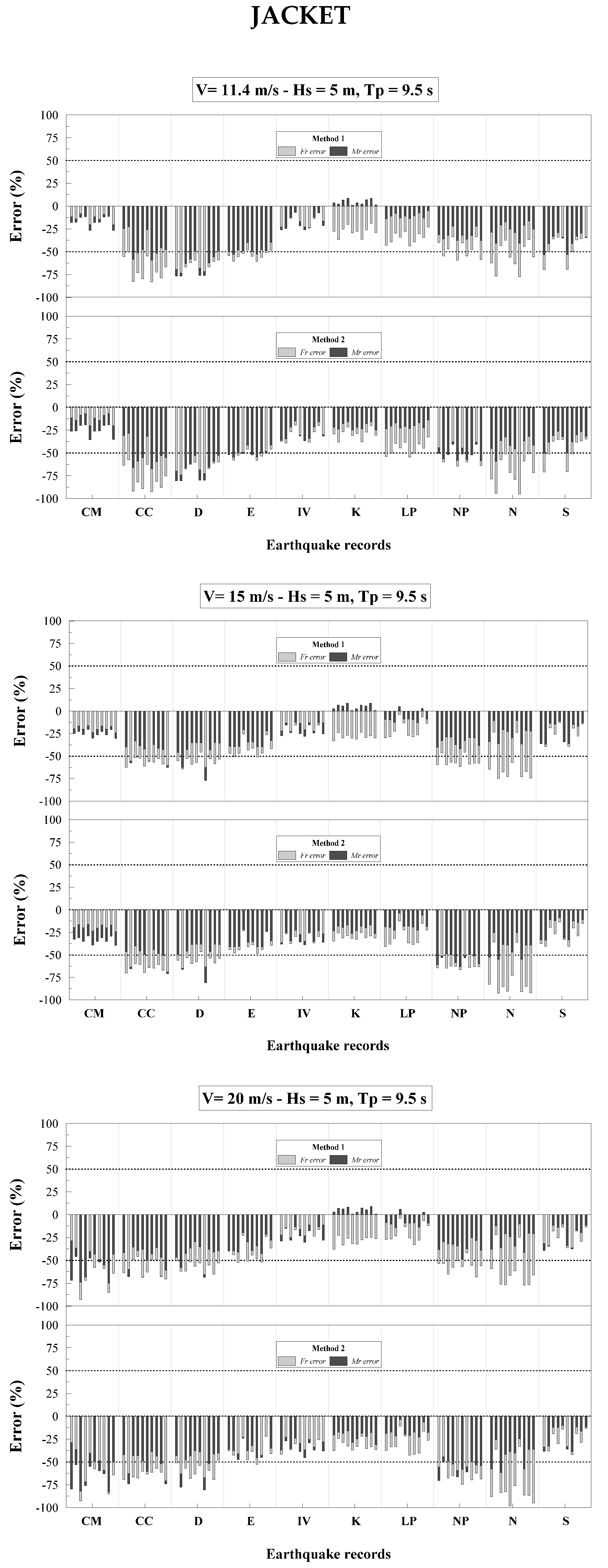
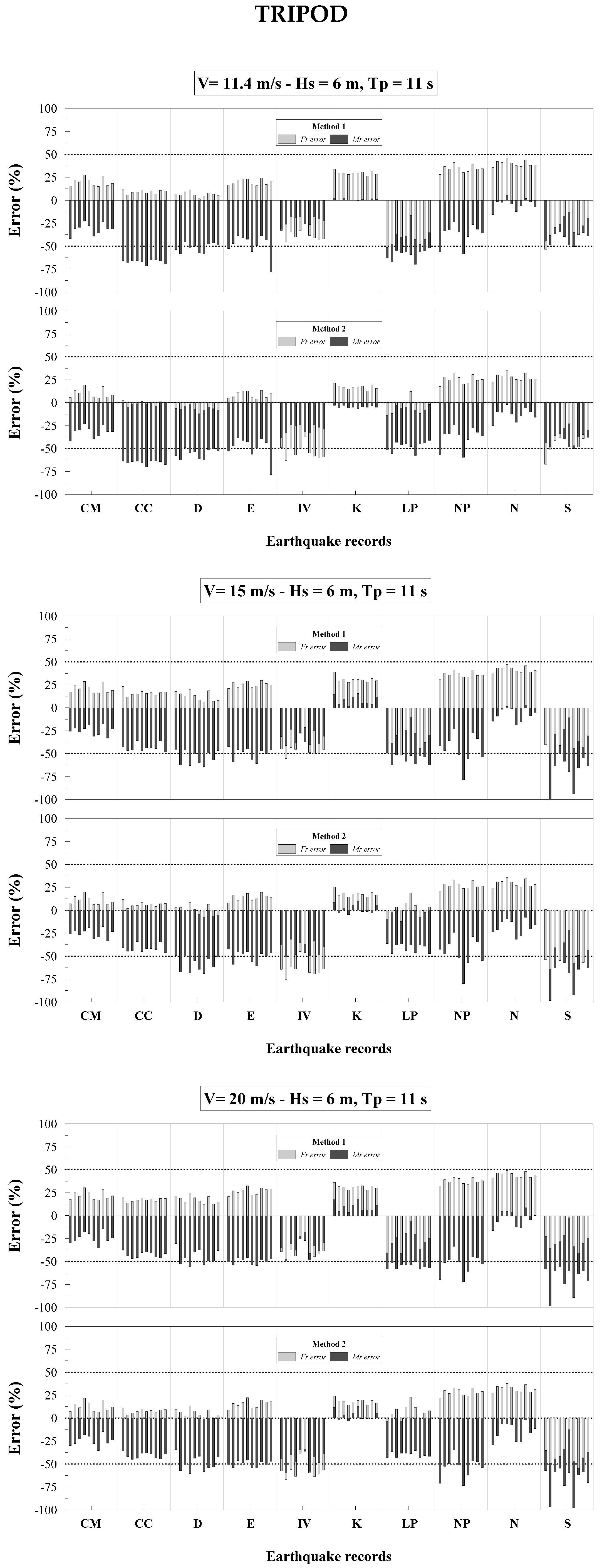
Errors (18) and (19) are reported in Figure 4, Figure 5, Figure 6 and Figure 7 for both Jacket and Tripod, as obtained from Methods 1-2 and fully-coupled simulations. Overall, 2 × 600 = 1200 fully-coupled simulations have been run to calculate and in Equations (1) and (2) (i.e., 600 for each support structure); 2 × (5 × 3) × (2 × 2) = 120 time-domain simulations under wind-waves only to calculate and in Equations (5) and (6) (i.e., (5 × 3) × (2 × 2) = 60 for each support structure, considering 5 wind samples for 3 wind velocities at the hub and 2 wave samples for 2 sea states); 2 × 10 = 20 FE response-spectrum analyses in Method 1 and 2 × 10 = 20 FE response-spectrum analyses in Method 2 to calculate and in Equations (7) and (8).
The first observation on Figure 4, Figure 5, Figure 6 and Figure 7 is that, in most cases, errors obtained by Method 1 and Method 2 are negative. However, errors may be positive for some earthquakes and wind-wave samples. This means that, although in most cases the stress-resultant demands obtained by Methods 1-2 are, as expected, larger than those from fully-coupled simulation (negative errors), there may be cases where they are smaller (positive errors), with the consequence that results are indeed non-conservative. A further observation on Figure 4, Figure 5, Figure 6 and Figure 7 is that positive errors by Methods 1-2 are definitely more numerous for the Tripod than the Jacket. For the Tripod, positive errors can be up to 50% in shear force and 20% in bending moment by Method 1, and up to 35% in shear force and 15% in bending moment by Method 2. For the Jacket, positive errors can be up to 10% in bending moment by Method 1, while no positive errors are encountered by Method 2. The fact that errors are may be significantly different for Jacket and Tripod is of particular interest, in recognition of the fact that the two structures exhibit very close natural frequencies, except for that of the 2nd support-structure modes in Table 1. This is evidence that accuracy of response-spectrum uncoupled analyses versus fully-coupled simulations is affected by mass and stiffness distribution of the support structure.
For a further insight into the results in Figure 4, Figure 5, Figure 6 and Figure 7, Table 4, Table 5, Table 6 and Table 7 report the mean demands at the tower base, as computed by averaging over the 5 × 2 = 10 wind-wave samples for every earthquake. It is seen that mean demands at the tower base may be smaller than those predicted by fully-coupled simulation (grey cells in Table 4, Table 5, Table 6 and Table 7). The fact that demands obtained by Methods 1-2 may be non-conservative, not only in terms of single samples (see Figure 4, Figure 5, Figure 6 and Figure 7) but also in terms of mean demands (Table 4, Table 5, Table 6 and Table 7), is an important conclusion of this study, and should possibly drive the selection of appropriate safety factors when applying response-spectrum uncoupled analyses for design purposes.
Results in Figure 4, Figure 5, Figure 6 and Figure 7 and Table 4, Table 5, Table 6 and Table 7 are obtained from Method 1 with N = 12 and Method 2 with N = 4 in Equations (10) and (12), using modes in Table 1 and corresponding modal damping ratios set in Section 3. It is noteworthy that results do not change appreciably if the number of modes increases. This is stated based on several numerical tests conducted in this study with up to N = 26 modes in Method 1 and N = 20 modes in Method 2, using again a 0.4775% damping ratio for blade modes and a 1% damping ratio for support-structure modes where, therefore, no aerodynamic damping effects have been considered. This assumption is consistent with numerical evidence [9,45,46] that 1st and 2nd support-structure modes in fore-aft direction are the support-structure modes that provide, in general, the main contribution to the earthquake response and where, accordingly, aerodynamic damping effects must be considered.
At this stage, an explanation for non-conservativeness of Methods 1-2 may be found in the fact that coupling among wind-wave-earthquake responses play a crucial role. Indeed, wind loads are strongly influenced by earthquake shaking at the base, as aerodynamic drag and lift forces on the rotor depend on the wind velocity relative to the blades. Earthquake shaking has the same influence on the hydrodynamic forces acting on the submerged support structure, as computed by Morison’s equation. All these effects cannot be taken into due account in uncoupled analyses where earthquake loads and wind-wave loads act separately on the system. In addition, it has to be noted that fully-coupled simulations implemented in GH-BLADED take into account active pitch control as well as nonlinearity arising from large displacements of the rotor with respect to the tower top. Therefore, based on the results in Figure 4, Figure 5, Figure 6 and Figure 7, it is concluded that even the rather conservative assumption made on the directional combination, i.e., that earthquake effects associated with the two horizontal components are added, see Equations (9) and (11), is not sufficient to compensate for the fact that separate analyses cannot adequately capture the inherent coupling among wind-wave-earthquake responses, as well as additional effects associated with active pitch control and large displacements of the rotor with respect to the tower top.
For a further insight into the feasibility of response-spectrum uncoupled analyses, finally a comparison is made between results from fully-coupled simulations and Method 3, i.e., the simplified approach prescribed by Annex C of IEC 61400-1 [12]. Therefore, as explained in Section 5.3, the maxima and of the separate earthquake response in Equations (3) and (4), obtained from an equivalent static analysis on FE Model 3 for every earthquake record in Table 3, are combined with the maxima and of the separate wind-wave response, built as characteristic values calculated from a single emergency-shutdown time-domain simulation on the Full Model at the rated wind speed [1,12].
Results in Table 8 and Table 9 reveal that also in this case response-spectrum uncoupled analyses may provide smaller demands than fully-coupled simulation being, therefore, non-conservative. This means that the fundamental assumptions of Annex C of IEC 61400-1 [12] may not be appropriate for offshore HAWTs. In details, the first assumption of Annex C is that the response is dominated by the 1st support-structure modes in fore-aft and side-to-side directions. Results in Table 8 and Table 9 show that this assumption is not adequate, confirming previous evidence that 2nd support-structure modes of the Jacket and Tripod under study are significantly excited by earthquake shaking [9]. On the other hand, Annex C does not account for blade modes that, instead, exhibit natural frequencies within the range of maxima response accelerations, see Figure 3. In this respect, similar conclusions have been drawn by other authors [34,47].
7. Conclusions
This paper has investigated three different methods of response-spectrum uncoupled analyses for seismic assessment of offshore wind turbines, based on International Standards and Guidelines prescriptions [1,2,3]. The methods differ in the structural models adopted and the criteria used to calculate the separate earthquake and wind-wave responses; among others, the simplified method suggested by Annex C of IEC 61400-1 [12] has been implemented. The case study is the baseline NREL 5-MW wind turbine [10], mounted on two typical support structures in intermediate waters, a jacket and a tripod, in 600 potential wind-wave-earthquake scenarios, which correspond to 3 wind velocities at the hub (each with 5 realizations), 2 sea states (each with 2 realizations) and 10 real earthquake records. To check accuracy, comparisons have been made with benchmark results obtained from time-domain, nonlinear fully-coupled simulations.
Numerical results have shown that all the considered response-spectrum uncoupled analyses, including the simplified method suggested by Annex C of IEC 61400-1 [12], may provide non-conservative results. Since this is found for all methods, irrespective of structural models adopted and criteria used to calculate earthquake and wind-wave responses, it is argued that non-conservativeness is essentially attributable to coupling as well as nonlinearities inherent in the combined wind-wave-earthquake response, which can be captured only by time-domain, nonlinear fully-coupled simulations. Based on the results of this paper, it is concluded that appropriate safety factors should be assumed when implementing response-spectrum uncoupled analyses for offshore wind turbines allowed by International Standards and Guidelines [1,2,3].
Finally, it is noteworthy that the results of this paper have been obtained for structural models clamped at the mudline. Because soil-structure interaction may play an important role in the seismic response of offshore HATWs, refined soil models appropriate for seismic response should be considered in future investigations. For instance, frequency-dependent springs/dashpots in parallel or springs/dashpots in series and parallel, including gap effects [48,49,50], could be considered for pile foundations. Including refined soil models for pile foundations in a response-spectrum approach, however, is a non-trivial task that will require pertinent approximations, especially when nonlinear behavior is involved. Soil-related nonlinearities may be accounted for, more easily, in time-domain uncoupled analyses, whose implementation has been discussed in a recent paper by the authors [35].
Author Contributions
Conceptualization, G.F. and F.A.; Methodology, G.F. and F.A.; Software, F.S., G.F. and F.S.; Validation, G.F., F.S., G.F. and F.S.; Investigation, G.F., F.S., G.F. and F.S.; Writing-Original Draft Preparation, G.F.; Writing-Review & Editing, G.F.; Supervision, G.F. and F.A.
Funding
This research received no external funding.
Conflicts of Interest
The authors declare no conflict of interest.
References
- International Electrotechnical Commission (IEC). Wind Turbines—Part 3: Design Requirements for Offshore Wind Turbines; IEC 61400-3; IEC: Geneva, Switzerland, 2009. [Google Scholar]
- Germanischer Lloyd (GL). Guideline for the Certification of Offshore Wind Turbines; GL 2012; GL: Hamburg, Germany, 2012. [Google Scholar]
- Det Norske Veritas (DNV). Design of Offshore Wind Turbine Structures; DNV-OS-J101; DNV: Copenhagen, Denmark, 2013. [Google Scholar]
- Failla, G.; Arena, F. New perspectives in offshore wind energy. Philos. Trans. R. Soc. Lond. Ser. A-Math. Phys. Eng. Sci. 2015, 373, 20140228. [Google Scholar] [CrossRef] [PubMed]
- Schwartz, M.; Heimiller, D.; Haymes, S.; Musial, W. Assessment of Offshore Wind Energy Resources for the United States; Report No. NREL/TP-500-45889; National Renewable Energy Laboratory (NREL): Golden, CO, USA, 2010.
- U.S. Geological Survey (USGS). Hazard Map (PGA, 2% in 50 Years); USGS: Reston, VA, USA, 2008. Available online: http://earthquake.usgs.gov/hazards/products (accessed on 1 March 2018).
- Haciefendioğlu, K. Stochastic seismic response analysis of offshore wind turbine including fluid-structure-soil-interaction. Struct. Des. Tall Spec. Build. 2012, 21, 867–878. [Google Scholar] [CrossRef]
- Kim, D.H.; Lee, S.G.; Lee, I.K. Seismic fragility analysis of 5 MW offshore wind turbine. Renew Energy 2014, 65, 250–256. [Google Scholar] [CrossRef]
- Alati, N.; Failla, G.; Arena, F. Seismic analysis of offshore wind turbines on bottom-fixed support structures. Philos. Trans. R. Soc. Lond. Ser. A-Math. Phys. Eng. Sci. 2015, 373, 20140086. [Google Scholar] [CrossRef] [PubMed]
- Jonkman, J.; Butterfield, S.; Musial, W.; Scott, G. Definition of a 5-MW Reference Wind Turbine for Offshore System Development; Report No. NREL/TP-500-38060; National Renewable Energy Laboratory (NREL): Golden, CO, USA, 2009.
- Katsanos, E.I.; Thöns, S.; Georgakis, C.Τ. Wind turbines and seismic hazard: A state-of-the-art review. Wind Energy 2016, 19, 2113–2133. [Google Scholar] [CrossRef]
- International Electrotechnical Commission (IEC). Wind Turbines—Part 1: Design Requirements; IEC 61400-1; IEC: Geneva, Switzerland, 2005. [Google Scholar]
- Germanischer Lloyd (GL). Guideline for the Certification of Wind Turbines; GL: Hamburg, Germany, 2010. [Google Scholar]
- American Society of Civil Engineers/American Wind Energy Association (ASCE/AWEA). Recommended Practice for Compliance of Large Land-Based Wind Turbine Support Structures; ASCE/AWEA RP2011; ASCE: Reston, VR, USA; AWEA: Washington, DC, USA, 2011. [Google Scholar]
- Wilson, E.L.; Der Kiureghian, A.; Bayo, E.P. A replacement for the srss method in seismic analysis. Earthq. Eng. Struct. Dyn. 1981, 9, 187–192. [Google Scholar] [CrossRef]
- Asareh, M.A.; Prowell, I. A simplified approach for implicitly considering aerodynamics in the seismic response of utility scale wind turbines. In Proceedings of the 53rd AIAA/ASME/ASCE/AHS/ASC Structures, Structural Dynamics and Materials Conference, Honolulu, HI, USA, 23–26 April 2012. [Google Scholar]
- Asareh, M.A.; Volz, J.S. Evaluation of aerodynamic and seismic coupling for wind turbines using finite element approach. In Proceedings of the ASME 2013 International Mechanical Engineering Congress and Exposition, San Diego, CA, USA, 15–21 November 2013. [Google Scholar]
- Santangelo, F.; Failla, G.; Santini, A.; Arena, F. Time-domain uncoupled analyses for seismic assessment of land-based wind turbines. Eng. Struct. 2016, 123, 275–299. [Google Scholar] [CrossRef]
- Valamanesh, V.; Myers, A. Aerodynamic damping and seismic response of horizontal axis wind turbine towers. J. Struct. Eng. 2014, 140, 04014090. [Google Scholar] [CrossRef]
- Witcher, D. Seismic analysis of wind turbines in the time domain. Wind Energy 2005, 8, 81–91. [Google Scholar] [CrossRef]
- Sadowski, A.J.; Camara, A.; Málaga-Chuquitaype, C.; Dai, K. Seismic analysis of a tall metal wind turbine support tower with realistic geometric imperfections. Earthq. Eng. Struct. Dyn. 2017, 46, 201–219. [Google Scholar] [CrossRef]
- Butt, U.A.; Ishihara, T. Seismic load evaluation of wind turbine support structures considering low structural damping and soil structure interaction. In Proceedings of the European Wind Energy Conference Exhibition (EWEC), Copenhagen, Denmark, 16–19 April 2012. [Google Scholar]
- Bossanyi, E.A. Bladed for Windows User Manual; Version 4.6; Garrad Hassan and Partners: Bristol, UK, 2000. [Google Scholar]
- Computers and Structures, Inc. Sap2000 Analysis Reference Manual; Version 14.0; Computers and Structures, Inc.: Berkeley, CA, USA, 2010. [Google Scholar]
- Agarwal, P.; Manuel, L. Incorporating irregular nonlinear waves in coupled simulation and reliability studies of offshore wind turbines. Appl. Ocean Res. 2011, 33, 215–227. [Google Scholar] [CrossRef]
- Nguyen, H.H.; Manuel, L. A Monte Carlo simulation study of wind turbine loads in thunderstorm downbursts. Wind Energy 2015, 18, 925–940. [Google Scholar] [CrossRef]
- Asareh, M.A.; Schonberg, W.; Volz, J. Effects of seismic and aerodynamic load interaction on structural dynamic response of multi-megawatt utility scale horizontal axis wind turbines. Renew. Energy 2016, 86, 49–58. [Google Scholar] [CrossRef]
- Kjørlaug, R.A.; Kaynia, A.M. Vertical earthquake response of megawatt-sized wind turbine with soil-structure interaction effects. Earthq. Eng. Struct. Dyn. 2015, 44, 2341–2358. [Google Scholar] [CrossRef]
- Avossa, A.M.; Demartino, C.; Contestabile, P.; Ricciardelli, F.; Vicinanza, D. Some results on the vulnerability assessment of HAWTs subjected to wind and seismic actions. Sustainability 2017, 9, 1525. [Google Scholar] [CrossRef]
- Avossa, A.M.; Demartino, C.; Ricciardelli, F. Assessment of the peak response of a 5MW HAWT under combined wind and seismic induced loads. Open Constr. Build. Technol. J. 2017, 11, 441–457. [Google Scholar] [CrossRef]
- Vorpahl, F.; Popko, W.; Kaufer, D. Description of a Basic Model of the ‘UpWind Reference Jacket’ for Code Comparison in the OC4 Project Under IEA Wind Annex 30; Technical Report; Fraunhofer Institute for Wind Energy and Energy System Technology IWES: Bremerhaven, Germany, 2013. [Google Scholar]
- Seidel, M. Jacket substructures for the REpower 5M wind turbine. In Proceedings of the Conference Proceedings European Offshore Wind, Berlin, Germany, 4–6 December 2007. [Google Scholar]
- Seidel, M.; Gosch, D. Technical challenges and their solution for the Beatrice windfarm demonstration project in 45m water depth. In Proceedings of the 8th German Wind Energy Conference (DEWEK), Bremen, Germany, 22–23 November 2006. [Google Scholar]
- Prowell, I.; Elgamal, A.; Uang, C.; Jonkman, J. Estimation of seismic load demand for a wind turbine in the time domain. In Proceedings of the European Wind Energy Conference Exhibition (EWEC), Warsaw, Poland, 20–23 April 2010. [Google Scholar]
- Santangelo, F.; Failla, G.; Arena, F.; Ruzzo, C. On time-domain uncoupled analyses for offshore wind turbines under seismic loads. Bull. Earthq. Eng. 2018, 16, 1007–1040. [Google Scholar] [CrossRef]
- Manwell, J.F.; McGowan, J.G.; Rogers, A.L. Wind Energy Explained: Theory, Design and Application; John Wiley & Sons: Chichester, UK, 2010. [Google Scholar]
- Chakrabarti, S.K. Hydrodynamics of Offshore Structures; WIT Press: Southampton, UK, 1987. [Google Scholar]
- Prowell, I. An Experimental and Numerical Study of Wind Turbine Seismic Behavior. Ph.D. Thesis, University of California, San Diego, CA, USA, 2011. [Google Scholar]
- Ishihara, T.; Yamaguchi, A.; Sarwar, M.W. A study of the normal turbulence model in IEC 61400-1. Wind Eng. 2012, 36, 759–766. [Google Scholar] [CrossRef]
- Ernst, B.; Seume, J.R. Investigation of site-specific wind field parameters and their effect on loads of offshore wind turbines. Energies 2012, 5, 3835–3855. [Google Scholar] [CrossRef]
- Leu, T.S.; Yo, J.M.; Tsai, Y.T.; Miau, J.J.; Wang, T.C. Assessment of IEC 61400-1 normal turbulence model for wind conditions in Taiwan west coast areas. Int. J. Mod. Phys. Conf. Ser. 2014, 34, 1460382. [Google Scholar] [CrossRef]
- Resor, B.R. Definition of a 5MW/61.5m Wind Turbine Blade Reference Model; Report No. SAND2013-2569; Wind Energy Technology Department Sandia National Laboratories: Albuquerque, NM, USA, 2013. [Google Scholar]
- Pacific Earthquake Engineering Research Center (PEER). Peer Ground Motion Database; PEER: Berkeley, CA, USA, 2013; Available online: http://ngawest2.berkeley.edu (accessed on 1 March 2018).
- Hasselmann, K.; Barnett, T.P.; Bouws, E.; Carlson, H.; Cartwright, D.E.; Enke, K.; Ewing, J.A.; Gienapp, H.; Hasselmann, D.E.; Kruseman, P.; et al. Measurements of wind wave growth and swell decay during the joint North Sea wave project (JONSWAP). Deutsche Hydrografische Zeitschrift 1973, A8, 1–95. [Google Scholar]
- Prowell, I.; Elgamal, A.; Uang, C.; Luco, J.E.; Romanowitz, H.; Duggan, E. Shake table testing and numerical simulation of a utility-scale wind turbine including operational effects. Wind Energy 2014, 17, 997–1016. [Google Scholar] [CrossRef]
- Díaz, O.; Suárez, L.E. Seismic analysis of wind turbines. Earthq. Spectra 2014, 30, 743–765. [Google Scholar] [CrossRef]
- Haenler, M.; Ritschel, U.; Warnke, I. Systematic modelling of wind turbine dynamics and earthquake loads on wind turbines. In Proceedings of the European Wind Energy Conference Exhibition (EWEC), Athens, Greece, 27 February–2 March 2006. [Google Scholar]
- Kavvadas, M.; Gazetas, G. Kinematic seismic response and bending of freehead piles in layered soil. Géotechnique 1993, 43, 207–222. [Google Scholar] [CrossRef]
- Makris, N.; Gazetas, G.; Delis, E. Dynamic soil-pile-foundation-structure interaction: Records and predictions. Géotechnique 1996, 46, 33–50. [Google Scholar] [CrossRef]
- Boulanger, R.W.; Curras, C.J.; Kutter, B.L.; Wilson, D.W.; Abghari, A. Seismic soil-pile-structure interaction experiments and analyses. J. Geotech. Geoenviron. Eng. 1999, 125, 750–759. [Google Scholar] [CrossRef]
Figure 1.
Test structures: (a) Jacket; (b) Tripod.

Figure 2.
Geometry of (a) Jacket and (b) Tripod (dimensions of structural members in mm; heights and depths in m).
Figure 2.
Geometry of (a) Jacket and (b) Tripod (dimensions of structural members in mm; heights and depths in m).

Figure 3.
5% damped spectral acceleration of earthquake records, as taken from ref. [43]; (a): x direction; (b) y direction.
Figure 3.
5% damped spectral acceleration of earthquake records, as taken from ref. [43]; (a): x direction; (b) y direction.

Figure 4.
Jacket: Tower base errors (18) and (19) obtained by Methods 1-2 for sea state parameters Hs = 5 m, Tp = 9.5 s, all wind velocities and earthquake records listed in Table 3.
Figure 4.
Jacket: Tower base errors (18) and (19) obtained by Methods 1-2 for sea state parameters Hs = 5 m, Tp = 9.5 s, all wind velocities and earthquake records listed in Table 3.

Figure 5.
Jacket: Tower base errors (18) and (19) obtained by Methods 1-2 for sea state parameters Hs = 6 m, Tp = 11 s, all wind velocities and earthquake records listed in Table 3.
Figure 5.
Jacket: Tower base errors (18) and (19) obtained by Methods 1-2 for sea state parameters Hs = 6 m, Tp = 11 s, all wind velocities and earthquake records listed in Table 3.

Figure 6.
Tripod: Tower base errors (18)–(19) obtained by Methods 1-2 for sea state parameters Hs = 5 m, Tp = 9.5 s, all wind velocities and earthquake records listed in Table 3.
Figure 6.
Tripod: Tower base errors (18)–(19) obtained by Methods 1-2 for sea state parameters Hs = 5 m, Tp = 9.5 s, all wind velocities and earthquake records listed in Table 3.

Figure 7.
Tripod: Tower base errors (18)–(19) obtained by Methods 1-2 for sea state parameters Hs = 6 m, Tp = 11 s, all wind velocities at hub and earthquake records listed in Table 3.
Figure 7.
Tripod: Tower base errors (18)–(19) obtained by Methods 1-2 for sea state parameters Hs = 6 m, Tp = 11 s, all wind velocities at hub and earthquake records listed in Table 3.


Table 1.
Natural frequencies of Full Model in GH-BLADED and FE Models 1-2 in SAP 2000.
| Jacket Frequencies (Hz) | Tripod Frequencies (Hz) | |||||
|---|---|---|---|---|---|---|
| Mode Description | GH BLADED Full Model | SAP 2000 FE Model 1 | SAP 2000 FE Model 2 | GH BLADED Full Model | SAP 2000 FE Model 1 | SAP 2000 FE Model 2 |
| 1st Supp. Struct. Side-to-Side | 0.314 | 0.325 | 0.345 | 0.309 | 0.319 | 0.321 |
| 1st Supp. Struct. Fore-Aft | 0.317 | 0.326 | 0.345 | 0.311 | 0.321 | 0.325 |
| 1st Blade Asym. Flapw. Yaw | 0.640 | 0.603 | - | 0.645 | 0.613 | - |
| 1st Blade Asym. Flapw. Pitch | 0.675 | 0.642 | - | 0.677 | 0.643 | - |
| 1st Blade Collective Flap | 0.708 | 0.690 | - | 0.710 | 0.695 | - |
| 1st Blade Asym. Edgew. Pitch | 1.080 | 1.095 | - | 1.081 | 1.030 | - |
| 1st Blade Asym. Edgew. Yaw | 1.092 | 1.104 | - | 1.097 | 1.105 | - |
| 2nd Blade Asym. Flapw. Yaw | 1.714 | 1.695 | - | 1.749 | 1.701 | - |
| 2nd Blade Asym. Flapw. Pitch | 1.937 | 1.899 | - | 1.848 | 1.805 | - |
| 2nd Blade Collective Flap | 2.003 | 1.952 | - | 1.996 | 1.905 | - |
| 2nd Supp. Struct. Fore-Aft | 1.241 | 1.287 | 1.228 | 2.206 | 2.242 | 2.321 |
| 2nd Supp. Struct. Side-to-Side | 1.219 | 1.201 | 1.228 | 2.277 | 2.320 | 2.327 |
Table 2.
Natural frequencies of two-degree-of-freedom FE Model 3.
| Jacket Frequencies (Hz) | Tripod Frequencies (Hz) | |
|---|---|---|
| Mode Description | SAP 2000 FE Model 3 | SAP 2000 FE Model 3 |
| Fore-Aft | 0.232 | 0.267 |
| Side-to-Side | 0.232 | 0.268 |
Table 3.
Earthquake records, wind velocities at the hub and sea states (PGA = peak ground acceleration).
Table 3.
Earthquake records, wind velocities at the hub and sea states (PGA = peak ground acceleration).
| Earthquake and Wind-Wave Loading | |||
|---|---|---|---|
| Earthquake Records | Year | Station | PGA (m/s2) |
| Cape Mendocino (CM) | 1992 | Petrolia | 6.12 |
| Chi Chi Taiwan (CC) | 1999 | TCU102 | 2.17 |
| Ducze-Turkey (D) | 1999 | Ducze | 4.23 |
| Erzican-Turkey (E) | 1992 | Erzican | 4.43 |
| Imperial Valley-06 (IV) | 1979 | E.C. #3 | 2.44 |
| Kobe-Japan (K) | 1995 | KJMA | 6.71 |
| Loma Prieta (LP) | 1989 | F.C.-APEEL 1 | 2.75 |
| N. Palm Springs (NP) | 1986 | N.P.S | 6.30 |
| Northridge (N) | 1994 | P.D.d. | 3.43 |
| Superstition Hills–01 (S) | 1987 | I.V. W.L.A. | 1.50 |
| Wind Velocities at Hub, V | Wind Samples | ||
| 11.4 m/s | 5 | ||
| 15 m/s | 5 | ||
| 20 m/s | 5 | ||
| Wave Periods and Significant Heights | Wave Samples | ||
| Hs = 5 m; Tp = 9.5 s | 2 | ||
| Hs = 6 m; Tp = 11 s | 2 | ||
Table 4.
Jacket: Mean shear-force and bending-moment demands at tower base, obtained by Methods 1-2 for sea state parameters Hs = 5 m, Tp = 9.5 s, all wind velocities and earthquake records listed in Table 3.
Table 4.
Jacket: Mean shear-force and bending-moment demands at tower base, obtained by Methods 1-2 for sea state parameters Hs = 5 m, Tp = 9.5 s, all wind velocities and earthquake records listed in Table 3.
| JACKET—Hs = 5 m, Tp = 9.5 s | |||||||||
|---|---|---|---|---|---|---|---|---|---|
| Mean Shear Force | |||||||||
| V = 11.4 m/s | V = 15 m/s | V = 20 m/s | |||||||
| EQ | Fully Coupled (MN) | Method 1 (MN) | Method 2 (MN) | Fully Coupled (MN) | Method 1 (MN) | Method 2 (MN) | Fully Couple (MN) | Method 1 (MN) | Method 2 (MN) |
| CM | 2.94 | 3.30 | 3.30 | 2.73 | 3.26 | 3.26 | 2.91 | 4.58 | 4.58 |
| CC | 2.74 | 4.62 | 4.86 | 2.91 | 4.58 | 4.82 | 2.90 | 4.53 | 4.68 |
| D | 2.25 | 3.72 | 3.74 | 2.38 | 3.68 | 3.70 | 2.28 | 3.60 | 3.69 |
| E | 2.60 | 4.01 | 3.94 | 2.82 | 3.97 | 3.90 | 2.73 | 3.91 | 3.78 |
| IV | 2.12 | 2.47 | 2.75 | 2.08 | 2.43 | 2.72 | 2.00 | 2.37 | 2.59 |
| K | 2.88 | 3.68 | 3.72 | 2.83 | 3.64 | 3.68 | 2.76 | 3.62 | 3.54 |
| LP | 1.98 | 2.66 | 2.86 | 2.20 | 2.62 | 2.82 | 2.17 | 2.51 | 2.76 |
| NP | 1.78 | 2.61 | 2.70 | 1.65 | 2.57 | 2.66 | 1.59 | 2.54 | 2.66 |
| N | 1.32 | 2.04 | 2.25 | 1.28 | 2.00 | 2.21 | 1.26 | 1.95 | 2.15 |
| S | 1.11 | 1.59 | 1.61 | 1.24 | 1.55 | 1.57 | 1.22 | 1.54 | 1.56 |
| Mean Bending Moment | |||||||||
| V = 11.4 m/s | V = 15 m/s | V = 20 m/s | |||||||
| EQ | Fully Coupled (MNm) | Method 1 (MNm) | Method 2 (MNm) | Fully Coupled (MNm) | Method 1 (MNm) | Method 2 (MNm) | Fully Coupled (MNm) | Method 1 (MNm) | Method 2 (MNm) |
| CM | 189.65 | 222.01 | 237.07 | 173.95 | 217.74 | 232.81 | 200.56 | 314.42 | 329.49 |
| CC | 208.72 | 296.86 | 311.61 | 201.18 | 292.59 | 307.34 | 193.78 | 281.76 | 306.73 |
| D | 143.66 | 235.24 | 240.29 | 162.10 | 230.97 | 236.02 | 160.36 | 225.13 | 224.40 |
| E | 166.15 | 245.75 | 248.40 | 181.11 | 241.48 | 244.13 | 173.63 | 236.86 | 235.43 |
| IV | 131.62 | 154.84 | 167.60 | 124.42 | 150.57 | 163.33 | 120.59 | 144.45 | 162.80 |
| K | 233.51 | 222.87 | 281.98 | 229.87 | 218.61 | 277.71 | 223.55 | 216.00 | 269.66 |
| LP | 160.00 | 176.96 | 192.19 | 161.41 | 172.69 | 187.92 | 159.06 | 172.32 | 181.97 |
| NP | 98.27 | 129.46 | 148.90 | 93.37 | 125.19 | 144.63 | 88.78 | 123.11 | 138.30 |
| N | 87.61 | 110.41 | 124.84 | 85.85 | 106.15 | 120.57 | 83.05 | 104.34 | 118.94 |
| S | 75.16 | 103.69 | 101.55 | 81.57 | 99.43 | 97.28 | 77.65 | 97.51 | 94.51 |
Table 5.
Jacket: Mean shear-force and bending-moment demands at tower base, obtained by Methods 1-2 for sea state parameters Hs = 6 m, Tp = 11 s, all wind velocities and earthquake records listed in Table 3.
Table 5.
Jacket: Mean shear-force and bending-moment demands at tower base, obtained by Methods 1-2 for sea state parameters Hs = 6 m, Tp = 11 s, all wind velocities and earthquake records listed in Table 3.
| JACKET—Hs = 6 m, Tp = 11 s | |||||||||
|---|---|---|---|---|---|---|---|---|---|
| Mean Shear Force | |||||||||
| V = 11.4 m/s | V = 15 m/s | V = 20 m/s | |||||||
| EQ | Fully Coupled (MN) | Method 1 (MN) | Method 2 (MN) | Fully Coupled (MN) | Method 1 (MN) | Method 2 (MN) | Fully Coupled (MN) | Method 1 (MN) | Method 2 (MN) |
| CM | 2.90 | 3.31 | 3.31 | 2.69 | 3.26 | 3.26 | 3.20 | 4.75 | 4.75 |
| CC | 2.75 | 4.63 | 4.87 | 2.92 | 4.58 | 4.82 | 2.80 | 4.54 | 4.79 |
| D | 2.24 | 3.73 | 3.74 | 2.37 | 3.68 | 3.70 | 2.32 | 3.67 | 3.66 |
| E | 2.60 | 4.01 | 3.95 | 2.81 | 3.97 | 3.90 | 2.79 | 3.90 | 3.72 |
| IV | 2.10 | 2.47 | 2.76 | 2.06 | 2.43 | 2.71 | 2.03 | 2.40 | 2.60 |
| K | 2.86 | 3.68 | 3.72 | 2.80 | 3.64 | 3.68 | 2.77 | 3.56 | 3.50 |
| LP | 1.97 | 2.66 | 2.86 | 2.21 | 2.61 | 2.82 | 2.11 | 2.51 | 2.69 |
| NP | 1.76 | 2.62 | 2.70 | 1.64 | 2.57 | 2.66 | 1.61 | 2.48 | 2.59 |
| N | 1.32 | 2.05 | 2.25 | 1.27 | 2.00 | 2.21 | 1.26 | 1.97 | 2.20 |
| S | 1.11 | 1.60 | 1.61 | 1.24 | 1.55 | 1.56 | 1.20 | 1.49 | 1.56 |
| Mean Bending Moment | |||||||||
| V = 11.4 m/s | V = 15 m/s | V = 20 m/s | |||||||
| EQ | Fully Coupled (MNm) | Method 1 (MNm) | Method 2 (MNm) | Fully Coupled (MNm) | Method 1 (MNm) | Method 2 (MNm) | Fully Coupled (MNm) | Method 1 (MNm) | Method 2 (MNm) |
| CM | 187.45 | 222.27 | 237.34 | 171.85 | 150.57 | 163.33 | 220.13 | 315.74 | 330.81 |
| CC | 211.66 | 297.12 | 311.88 | 204.37 | 217.91 | 232.98 | 201.85 | 291.79 | 300.12 |
| D | 144.37 | 235.50 | 240.55 | 163.07 | 292.76 | 307.52 | 155.68 | 228.28 | 233.47 |
| E | 165.17 | 246.01 | 248.67 | 181.19 | 231.14 | 236.19 | 175.18 | 233.76 | 244.22 |
| IV | 131.73 | 155.10 | 167.86 | 124.36 | 241.65 | 244.30 | 120.21 | 147.16 | 160.73 |
| K | 233.71 | 223.14 | 282.25 | 230.07 | 218.78 | 277.88 | 228.88 | 217.84 | 265.62 |
| LP | 159.47 | 177.22 | 192.45 | 161.35 | 172.86 | 188.09 | 156.98 | 165.47 | 180.43 |
| NP | 97.79 | 129.73 | 149.16 | 92.77 | 125.36 | 144.80 | 88.53 | 122.13 | 138.44 |
| N | 86.97 | 110.68 | 125.10 | 85.00 | 106.32 | 120.74 | 81.35 | 101.68 | 119.02 |
| S | 75.28 | 103.96 | 101.81 | 81.50 | 99.60 | 97.45 | 78.85 | 95.53 | 92.79 |
Table 6.
Tripod: Mean shear-force and bending-moment demands at tower base, obtained by Methods 1-2 for sea state parameters Hs = 5 m, Tp = 9.5 s, all wind velocities and earthquake records listed in Table 3.
Table 6.
Tripod: Mean shear-force and bending-moment demands at tower base, obtained by Methods 1-2 for sea state parameters Hs = 5 m, Tp = 9.5 s, all wind velocities and earthquake records listed in Table 3.
| TRIPOD—Hs = 5 m, Tp = 9.5 s | |||||||||
|---|---|---|---|---|---|---|---|---|---|
| Mean Shear Force | |||||||||
| V = 11.4 m/s | V = 15 m/s | V = 20 m/s | |||||||
| EQ | Fully Coupled (MN) | Method 1 (MN) | Method 2 (MN) | Fully Coupled (MN) | Method 1 (MN) | Method 2 (MN) | Fully Coupled (MN) | Method 1 (MN) | Method 2 (MN) |
| CM | 13.29 | 9.75 | 10.90 | 13.00 | 9.30 | 10.44 | 12.80 | 9.06 | 10.20 |
| CC | 11.67 | 9.34 | 10.36 | 11.45 | 8.89 | 9.91 | 11.40 | 8.65 | 9.67 |
| D | 12.07 | 10.08 | 11.49 | 12.03 | 9.62 | 11.03 | 12.25 | 9.38 | 10.79 |
| E | 11.94 | 8.87 | 10.12 | 12.27 | 8.42 | 9.66 | 11.93 | 8.18 | 9.42 |
| IV | 5.65 | 7.32 | 8.21 | 5.49 | 6.87 | 7.75 | 5.58 | 6.63 | 7.51 |
| K | 16.10 | 11.67 | 13.78 | 15.95 | 11.22 | 13.33 | 15.58 | 10.98 | 13.09 |
| LP | 7.38 | 9.79 | 7.37 | 7.81 | 9.34 | 6.91 | 7.91 | 9.09 | 6.67 |
| NP | 18.31 | 11.06 | 12.62 | 17.86 | 10.60 | 12.17 | 17.81 | 10.36 | 11.93 |
| N | 15.40 | 8.45 | 10.18 | 15.28 | 8.00 | 9.72 | 15.40 | 7.76 | 9.48 |
| S | 4.67 | 5.28 | 5.75 | 4.19 | 4.83 | 5.30 | 4.33 | 4.58 | 5.06 |
| Mean Bending Moment | |||||||||
| V = 11.4 m/s | V = 15 m/s | V = 20 m/s | |||||||
| EQ | Fully Coupled (MNm) | Method 1 (MNm) | Method 2 (MNm) | Fully Coupled (MNm) | Method 1 (MNm) | Method 2 (MNm) | Fully Coupled (MNm) | Method 1 (MNm) | Method 2 (MNm) |
| CM | 286.96 | 361.11 | 361.46 | 243.52 | 289.96 | 290.31 | 234.30 | 278.12 | 278.47 |
| CC | 320.72 | 463.58 | 458.58 | 245.92 | 392.43 | 387.44 | 245.61 | 380.59 | 375.59 |
| D | 270.17 | 396.61 | 405.88 | 216.96 | 325.47 | 334.73 | 225.95 | 313.62 | 322.89 |
| E | 284.61 | 399.84 | 399.92 | 224.80 | 328.69 | 328.77 | 215.83 | 316.85 | 316.93 |
| IV | 249.70 | 297.66 | 312.73 | 181.26 | 226.51 | 241.58 | 168.79 | 214.67 | 229.74 |
| K | 397.09 | 387.05 | 408.07 | 363.04 | 315.90 | 336.93 | 360.68 | 304.06 | 325.08 |
| LP | 221.29 | 338.93 | 314.39 | 174.24 | 267.78 | 243.25 | 167.17 | 255.94 | 231.40 |
| NP | 220.74 | 277.97 | 279.61 | 163.15 | 206.82 | 208.46 | 141.62 | 194.98 | 196.62 |
| N | 284.70 | 277.64 | 299.72 | 209.39 | 206.49 | 228.58 | 209.98 | 194.65 | 216.73 |
| S | 173.08 | 234.01 | 232.85 | 110.03 | 162.86 | 161.70 | 97.78 | 151.02 | 149.86 |
Table 7.
Tripod: Mean shear-force and bending-moment demands at tower base, obtained by Methods 1-2 for sea state parameters Hs = 6 m, Tp = 11 s, all wind velocities and earthquake records listed in Table 3.
Table 7.
Tripod: Mean shear-force and bending-moment demands at tower base, obtained by Methods 1-2 for sea state parameters Hs = 6 m, Tp = 11 s, all wind velocities and earthquake records listed in Table 3.
| TRIPOD—Hs = 6 m, Tp = 11 s | |||||||||
|---|---|---|---|---|---|---|---|---|---|
| Mean Shear Force | |||||||||
| V = 11.4 m/s | V = 15 m/s | V = 20 m/s | |||||||
| EQ | Fully Coupled (MN) | Method 1 (MN) | Method 2 (MN) | Fully Coupled (MN) | Method 1 (MN) | Method 2 (MN) | Fully Coupled (MN) | Method 1 (MN) | Method 2 (MN) |
| CM | 13.52 | 9.85 | 10.99 | 13.06 | 9.39 | 10.54 | 13.05 | 9.15 | 10.30 |
| CC | 10.62 | 9.44 | 10.46 | 10.96 | 8.98 | 10.00 | 10.85 | 8.74 | 9.76 |
| D | 11.34 | 10.17 | 11.58 | 12.07 | 9.72 | 11.13 | 12.47 | 9.48 | 10.89 |
| E | 11.81 | 8.97 | 10.21 | 12.12 | 8.51 | 9.76 | 12.17 | 8.27 | 9.52 |
| IV | 6.06 | 7.42 | 8.31 | 5.74 | 6.96 | 7.85 | 5.70 | 6.72 | 7.61 |
| K | 17.65 | 11.77 | 13.88 | 17.27 | 11.32 | 13.42 | 17.28 | 11.07 | 13.18 |
| LP | 8.49 | 9.89 | 7.46 | 8.60 | 9.43 | 7.01 | 8.71 | 9.19 | 6.77 |
| NP | 18.81 | 11.16 | 12.72 | 18.24 | 10.70 | 12.27 | 17.92 | 10.46 | 12.02 |
| N | 15.76 | 8.55 | 10.27 | 15.15 | 8.10 | 9.82 | 15.29 | 7.85 | 9.58 |
| S | 4.76 | 5.38 | 5.85 | 4.45 | 4.92 | 5.40 | 4.58 | 4.68 | 5.15 |
| Mean Bending Moment | |||||||||
| V = 11.4 m/s | V = 15 m/s | V = 20 m/s | |||||||
| EQ | Fully Coupled (MNm) | Method 1 (MNm) | Method 2 (MNm) | Fully Coupled (MNm) | Method 1 (MNm) | Method 2 (MNm) | Fully Coupled (MNm) | Method 1 (MNm) | Method 2 (MNm) |
| CM | 290.89 | 359.39 | 359.74 | 244.93 | 288.24 | 288.59 | 241.55 | 276.40 | 276.75 |
| CC | 280.01 | 461.86 | 456.86 | 287.23 | 390.71 | 385.72 | 273.37 | 378.87 | 373.87 |
| D | 270.18 | 394.89 | 404.16 | 220.76 | 323.75 | 333.01 | 237.15 | 311.90 | 321.17 |
| E | 286.86 | 398.12 | 398.20 | 224.14 | 326.97 | 327.05 | 214.64 | 315.13 | 315.21 |
| IV | 250.32 | 295.94 | 311.01 | 180.42 | 224.79 | 239.86 | 167.69 | 212.95 | 228.02 |
| K | 393.19 | 385.33 | 406.35 | 372.06 | 314.18 | 335.21 | 370.56 | 302.34 | 323.36 |
| LP | 221.88 | 337.21 | 312.67 | 175.13 | 266.06 | 241.53 | 169.72 | 254.22 | 229.68 |
| NP | 221.77 | 276.25 | 277.89 | 164.85 | 205.10 | 206.74 | 143.01 | 193.26 | 194.90 |
| N | 290.27 | 275.92 | 298.00 | 210.80 | 204.77 | 226.86 | 211.16 | 192.93 | 215.01 |
| S | 171.60 | 232.29 | 231.13 | 158.83 | 161.14 | 159.98 | 94.33 | 149.30 | 148.14 |
Table 8.
Jacket: Shear-force and bending-moment demands at tower base, obtained by Method 3 for emergency shutdown at rated wind speed V = 11.4 m/s and all earthquake records listed in Table 3.
Table 8.
Jacket: Shear-force and bending-moment demands at tower base, obtained by Method 3 for emergency shutdown at rated wind speed V = 11.4 m/s and all earthquake records listed in Table 3.
| JACKET | ||||||
|---|---|---|---|---|---|---|
| Hs = 5 m, Tp = 9.5 s | Hs = 6 m, Tp = 11 s | |||||
| Maximum Shear Force | ||||||
| EQ | Fully Coupled (MN) | Annex C (MN) | Error (%) | Fully Coupled (MN) | Annex C (MN) | Error (%) |
| CM | 3.04 | 2.42 | 20.39 | 2.98 | 2.43 | 18.45 |
| CC | 2.53 | 6.91 | −173.12 | 2.52 | 6.92 | −174.60 |
| D | 2.23 | 4.37 | −95.96 | 2.24 | 4.39 | −95.98 |
| E | 2.58 | 2.75 | −6.58 | 2.57 | 2.76 | −7.39 |
| IV | 2.17 | 2.61 | −20.27 | 2.16 | 2.63 | −21.75 |
| K | 2.93 | 2.34 | 20.13 | 2.95 | 2.35 | 20.33 |
| LP | 2.04 | 2.15 | −5.39 | 2.03 | 2.16 | −6.40 |
| NP | 1.77 | 1.66 | 6.21 | 1.74 | 1.68 | 3.44 |
| N | 1.42 | 1.61 | −13.38 | 1.40 | 1.62 | −15.71 |
| S | 1.16 | 1.79 | −54.31 | 1.16 | 1.80 | −55.17 |
| Maximum Bending Moment | ||||||
| EQ | Fully Coupled (MNm) | Annex C (MNm) | Error (%) | Fully Coupled (MNm) | Annex C (MNm) | Error (%) |
| CM | 198.08 | 165.84 | 16.27 | 195.09 | 165.47 | 15.18 |
| CC | 187.77 | 471.25 | −150.97 | 187.20 | 470.87 | −151.53 |
| D | 144.55 | 298.73 | −106.66 | 146.92 | 298.35 | −103.06 |
| E | 165.71 | 188.01 | −13.45 | 165.26 | 187.64 | −13.54 |
| IV | 138.21 | 179.05 | −29.54 | 138.59 | 178.67 | −28.91 |
| K | 239.11 | 160.63 | 32.82 | 239.74 | 160.26 | 33.15 |
| LP | 164.41 | 147.61 | 10.21 | 164.14 | 147.24 | 10.29 |
| NP | 98.40 | 114.42 | −16.28 | 97.46 | 114.04 | −17.01 |
| N | 91.71 | 110.78 | −20.79 | 91.03 | 110.40 | −21.27 |
| S | 77.91 | 122.90 | −57.74 | 77.93 | 122.53 | −57.23 |
Table 9.
Tripod: Shear-force and bending-moment demands at tower base, obtained by Method 3 for emergency shutdown at rated wind speed V = 11.4 m/s and all earthquake records listed in Table 3.
Table 9.
Tripod: Shear-force and bending-moment demands at tower base, obtained by Method 3 for emergency shutdown at rated wind speed V = 11.4 m/s and all earthquake records listed in Table 3.
| TRIPOD | ||||||
|---|---|---|---|---|---|---|
| Hs = 5 m, Tp = 9.5 s | Hs = 6 m, Tp = 11 s | |||||
| Maximum Shear Force | ||||||
| EQ | Fully Coupled (MN) | Annex C (MN) | Error (%) | Fully Coupled (MN) | Annex C (MN) | Error (%) |
| CM | 12.71 | 5.27 | 58.53 | 11.56 | 5.36 | 53.63 |
| CC | 10.50 | 6.07 | 42.19 | 10.62 | 6.17 | 41.90 |
| D | 10.77 | 6.71 | 37.69 | 10.83 | 6.80 | 37.21 |
| E | 11.35 | 5.95 | 47.57 | 10.70 | 6.05 | 43.45 |
| IV | 5.08 | 5.19 | −2.16 | 5.53 | 5.28 | 4.52 |
| K | 15.76 | 5.41 | 65.67 | 17.65 | 5.50 | 68.83 |
| LP | 7.36 | 5.35 | 27.31 | 6.49 | 5.44 | 16.17 |
| NP | 17.25 | 5.08 | 70.55 | 15.39 | 5.18 | 66.34 |
| N | 14.52 | 4.52 | 68.87 | 13.16 | 4.61 | 64.96 |
| S | 4.42 | 4.55 | −2.94 | 3.46 | 4.65 | −34.39 |
| Maximum Bending Moment | ||||||
| EQ | Fully Coupled (MNm) | Annex C (MNm) | Error (%) | Fully Coupled (MNm) | Annex C (MNm) | Error (%) |
| CM | 269.54 | 362.73 | −34.57 | 251.93 | 364.54 | −44.69 |
| CC | 294.19 | 442.77 | −50.50 | 277.47 | 444.58 | −60.22 |
| D | 244.67 | 505.91 | −106.77 | 255.02 | 507.72 | −99.09 |
| E | 257.99 | 430.73 | −66.95 | 259.29 | 432.54 | −66.81 |
| IV | 227.81 | 355.09 | −55.87 | 223.04 | 356.90 | −60.01 |
| K | 381.79 | 376.95 | 1.26 | 393.10 | 378.76 | 3.64 |
| LP | 209.12 | 370.81 | −77.31 | 205.20 | 372.62 | −81.58 |
| NP | 182.07 | 344.81 | −89.38 | 175.57 | 346.62 | −97.42 |
| N | 252.09 | 288.53 | −14.45 | 236.76 | 290.34 | −22.63 |
| S | 156.46 | 292.16 | −86.73 | 158.83 | 293.97 | −85.08 |
© 2018 by the authors. Licensee MDPI, Basel, Switzerland. This article is an open access article distributed under the terms and conditions of the Creative Commons Attribution (CC BY) license (http://creativecommons.org/licenses/by/4.0/).
Share and Cite
MDPI and ACS Style
Failla, G.; Santangelo, F.; Foti, G.; Scali, F.; Arena, F. Response-Spectrum Uncoupled Analyses for Seismic Assessment of Offshore Wind Turbines. J. Mar. Sci. Eng. 2018, 6, 85. https://doi.org/10.3390/jmse6030085
AMA Style
Failla G, Santangelo F, Foti G, Scali F, Arena F. Response-Spectrum Uncoupled Analyses for Seismic Assessment of Offshore Wind Turbines. Journal of Marine Science and Engineering. 2018; 6(3):85. https://doi.org/10.3390/jmse6030085
Chicago/Turabian StyleFailla, Giuseppe, Fabio Santangelo, Gabriele Foti, Fabio Scali, and Felice Arena. 2018. "Response-Spectrum Uncoupled Analyses for Seismic Assessment of Offshore Wind Turbines" Journal of Marine Science and Engineering 6, no. 3: 85. https://doi.org/10.3390/jmse6030085
Note that from the first issue of 2016, this journal uses article numbers instead of page numbers. See further details here.