Article

Effects of Harbor Shape on the Induced Sedimentation; L-Type Basin

by
Rozita Kian
1,*,†,
Deniz Velioglu
2,‡,
Ahmet Cevdet Yalciner
2,‡ and
Andrey Zaytsev
3,‡
1
Ocean Engineering Department, University of Rhode Island, Narragansett, RI 02882, USA
2
Civil Engineering Department, Middle East Technical University, Ankara 06800, Turkey
3
Special Research Bureau for Automation of Marine Researches, Far Eastern Branch of Russian Academy of Sciences, Uzhno-Sakhalinsk 693013, Russia
*
Author to whom correspondence should be addressed.
J. Mar. Sci. Eng. 2016, 4(3), 55; https://doi.org/10.3390/jmse4030055
Submission received: 18 July 2016 / Revised: 22 August 2016 / Accepted: 24 August 2016 / Published: 2 September 2016

Abstract

:
Tsunamis in shallow water zones lead to sea water level rise and fall, strong currents, forces (drag, impact, uplift, etc.), morphological changes (erosion, deposition), dynamic water pressure, as well as resonant oscillations. As a result, ground materials under the tsunami motion move, and scour/erosion/deposition patterns can be observed in the region. Ports and harbors as enclosed basins are the main examples of coastal structures that usually encounter natural hazards with small or huge damaging scales. Morphological changes are one of the important phenomena in the basins under short and long wave attack. Tsunamis as long waves lead to sedimentation in the basins, and therefore, in this study, the relation to the current pattern is noticed to determine sedimentation modes. Accordingly, we present a methodology based on the computation of the instantaneous Rouse number to investigate the tsunami motion and to calculate the respective sedimentation. This study aims to investigate the effects of the incident wave period on an L-type harbor sedimentation with a flat bathymetry using a numerical tool, NAMI DANCE, which solves non-linear shallow water equations. The results showed that the corner points on the bending part of the basin are always the critical points where water surface elevation and current velocity amplify in the exterior and interior corners, respectively.

1. Introduction

Ocean waves cannot generate enough energy to affect open coasts by resonance amplification, yet they can cause hazardous oscillations as they enter the enclosed or semi-enclosed basins and harbors. Tsunamis are known to be a very destructive phenomenon in shallow water, leading to sea water level rise and fall, strong currents, scour and morphological changes (erosion, deposition), resonant oscillations and seiches [1,2]. Wave radiation via the semi-enclosed basins is an important factor in decaying energy. Nonetheless, making the harbor entrance narrower results in the amplification of arriving wave. In fact, both harbor resonance period and harbor damage parameters can be related by harbor structures’ design determining the harbor geometry [3]. Generally, wave disturbance is a major factor in harbor design assumptions [4]. Breakwaters are capable of protecting the harbors against short waves [5], but the ability of long waves (with 25–300-s periods) in entering the harbors makes it often beyond control and causes oscillation problems [6,7,8]. Periods of oscillations can be in the range of a few seconds to a few minutes depending on the harbor geometry [9,10]. Several regular-shaped basins have been simulated to determine the first and the second mode of free oscillations of the basins, such as the L-type basin in [11]. The current study investigates the effect of wave period on the estimation of tsunami evolution, propagation and amplification, as well as tsunami currents and morphology changes in L-type basins with flat bathymetry. Here, a methodology is presented based on the computation of the instantaneous Rouse number [12] during tsunami simulation to investigate the tsunami motion and to determine the mode of the sediment transport. This is by computing the spatial and temporal change of the Rouse number under tsunami inundation according to the approach given in [13]. Accordingly, the numerical model NAMI DANCE [14] is employed to study the oscillations and amplification of waves and currents, as well as sediment motions in a harbor of the L shape with a flat bathymetry. This numerical tool has been developed by the C++ programming language using the leap-frog scheme numerical solution procedure. It utilizes the finite difference computational method to solve linear and nonlinear forms of depth-averaged shallow water equations in long wave problems. Since some natural harbors can be in the L shape after smoothing, here we investigate the current amplification and sediment movement in L-type basins for several free oscillation periods. It is observed that the corner points in the bending part of L-type basins are the critical points where the wave amplitude and current velocity amplify in basin free oscillation wave periods. Furthermore, the exposed sediment motion can be categorized according to the Rouse number values.

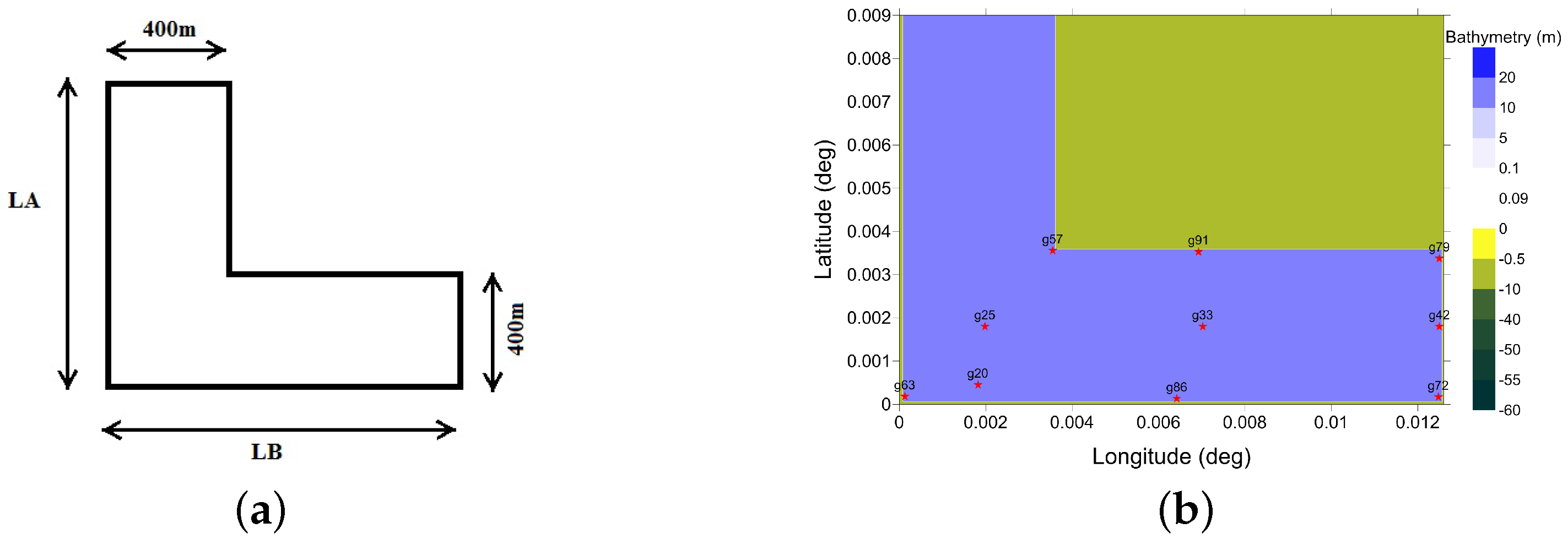
2. Materials and Methods

2.1. Rouse Number

The sediment motion can be observed by monitoring the spatial and temporal changes of the Rouse number. The Rouse number is a dimensionless number for classifying the modes of sediment transport [13]. It is defined as the ratio of particle settling velocity to the shear velocity:
R 0 = w s β κ u *
where u * is the shear velocity, β denotes the ratio of sediment diffusion to momentum diffusion coefficients (approximately equal to 1), κ is the von Karman constant (equal to 0.4) and settling velocity w s is given by [13]:
w s = 8 ν d 1 + ( s - 1 ) g d 3 72 ν 2 - 1
where s is the density of sand in water, i.e., the ratio of sediment density to water density ( ρ s /ρ), d represents the mean grain size, g is gravitational acceleration, ν denotes kinematic viscosity and u * is the shear velocity and can be written according to Equation (3) [13].
u * = u f 8
where f is the Darcy friction factor in the range of (0.006–0.039), and it is generally assumed to be equal to 0.01 in tsunami cases [13]. The mean grain size (d) for the entire domain is assumed 0.3 mm, which is a close value to the real cases (i.e., Belek area [15,16]). The values for the constants required for settling velocity and shear velocity calculations are listed in Table 1.
Modes of the sediment transport can be determined according to the Rouse number values. Sediment transport modes are in the form of bed load, suspended load and wash load (Table 2). Rouse number values greater than 2.5 represent the bed load form of sediment motion, while a value less than 0.8 is the mode of wash load sediment motion fully supported by the flow. Large values of the Rouse number indicate slower sediment motion and less severe erosion or deposition. On the other hand, smaller values of the Rouse number show more severe erosion in the topography.

2.2. Numerical Model

The effect of wave period on tsunami-induced sedimentation in the L-type basins is investigated using NAMI DANCE code. The governing equations of NAMI DANCE are the nonlinear form of shallow water equations. The schematic form of the basin in the simulations and 10 selected gauge points is illustrated in Figure 1. Depicted in Figure 1a are the metric dimensions of the basin, while Figure 1b shows the dimensions in the geographical outline (longitude-latitude) used in NAMI DANCE simulations. Initially, 100 gauge points are selected out of which 10 points are presented here. The bathymetry is flat, and the water depth is 20 m. LA in Figure 1a is the vertical dimension, and LB is the horizontal dimension of the basin. In half of the simulations, LA and LB are both used as 1000 m and another half of LA is 800 m (by placing the input source 200 m from the border), while LB is kept constant as 1000 m. The bending side is used as 400 m, and the grid size ( Δ x ) and time step ( Δ t ) are selected as 2 m and 0.005 s, respectively in all simulations. The input waves are in the form of several sinusoidal functions. They are sinusoidal crest lines entering parallel to the horizontal side (B side) from the basin entrance (400 m opening in the A side). The input waves are considered to have a 1-m amplitude with several random periods (16 s, 46 s, 90 s, 146 s and 328 s). Among those, 328 s, 146 s and 90 s are the second, fourth and seventh modes of the basin free oscillations [17], respectively. The differences of harbor modes for LA/LB = 0.8 and LA/LB = 1 are negligible (less than 5 s), and hence, they are only presented for the L-type basin with LA/LB = 1 dimensions in [17]. The boundaries are set with a 20-m wall; therefore, they perform as reflective, where their effects are considered in the next waves during the simulations after the first wave reaches the boundaries. It is worth mentioning that all simulations are performed for 40 min.

3. Results

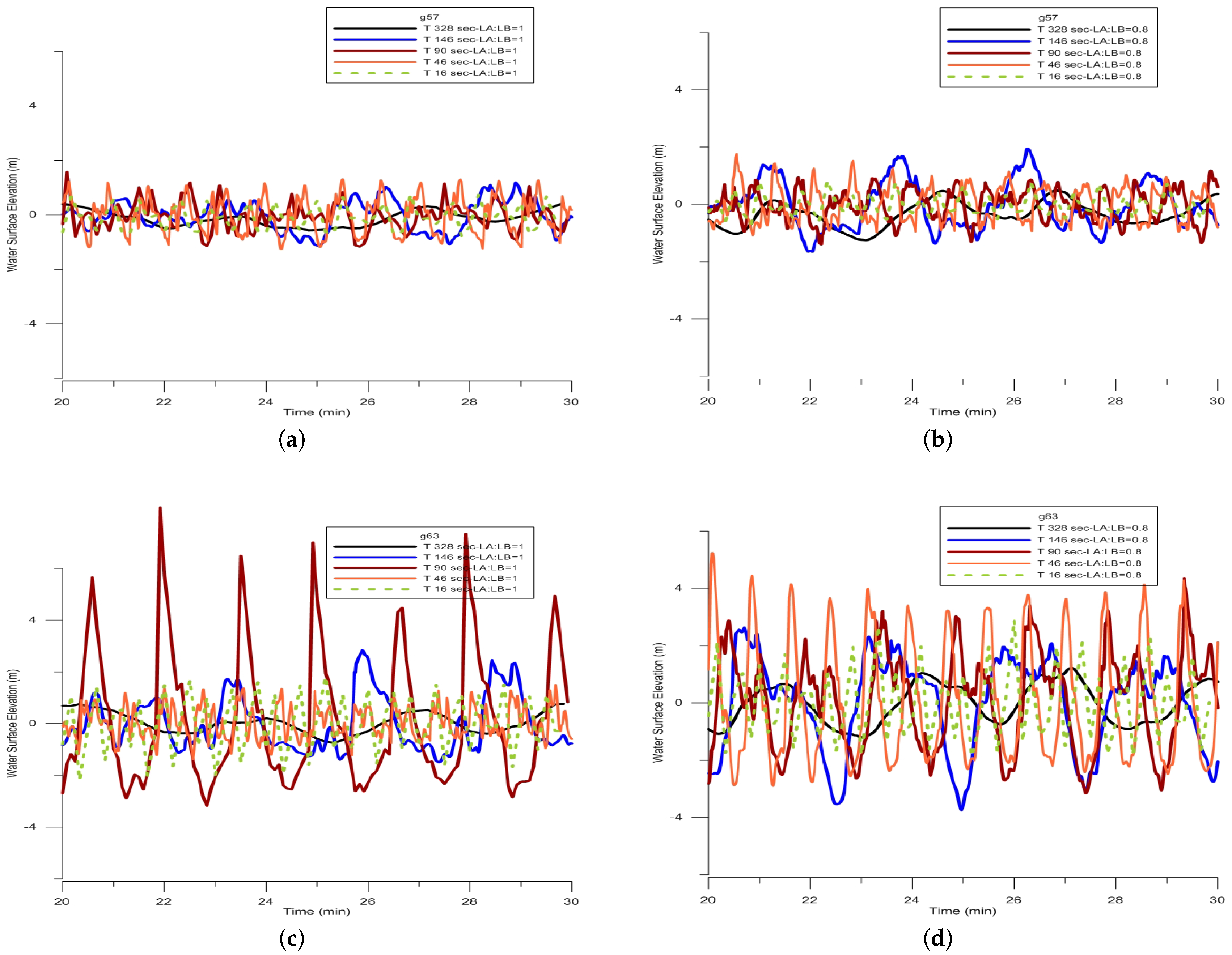
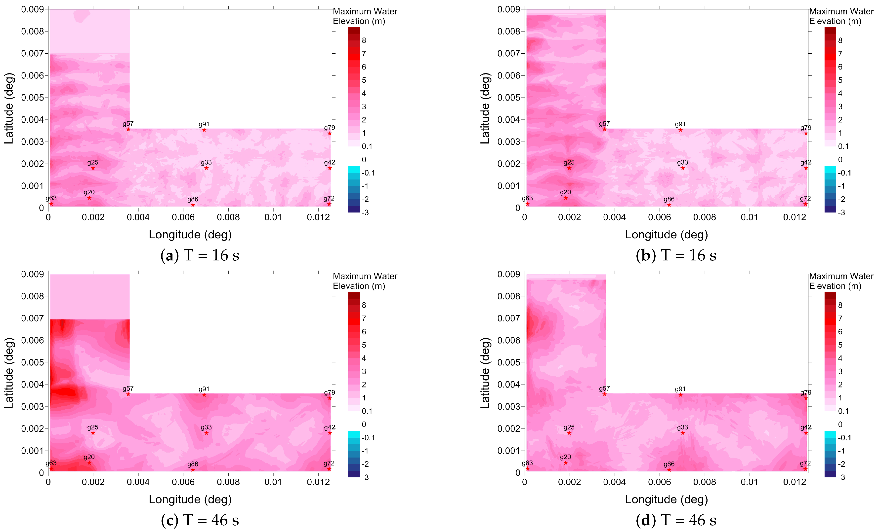
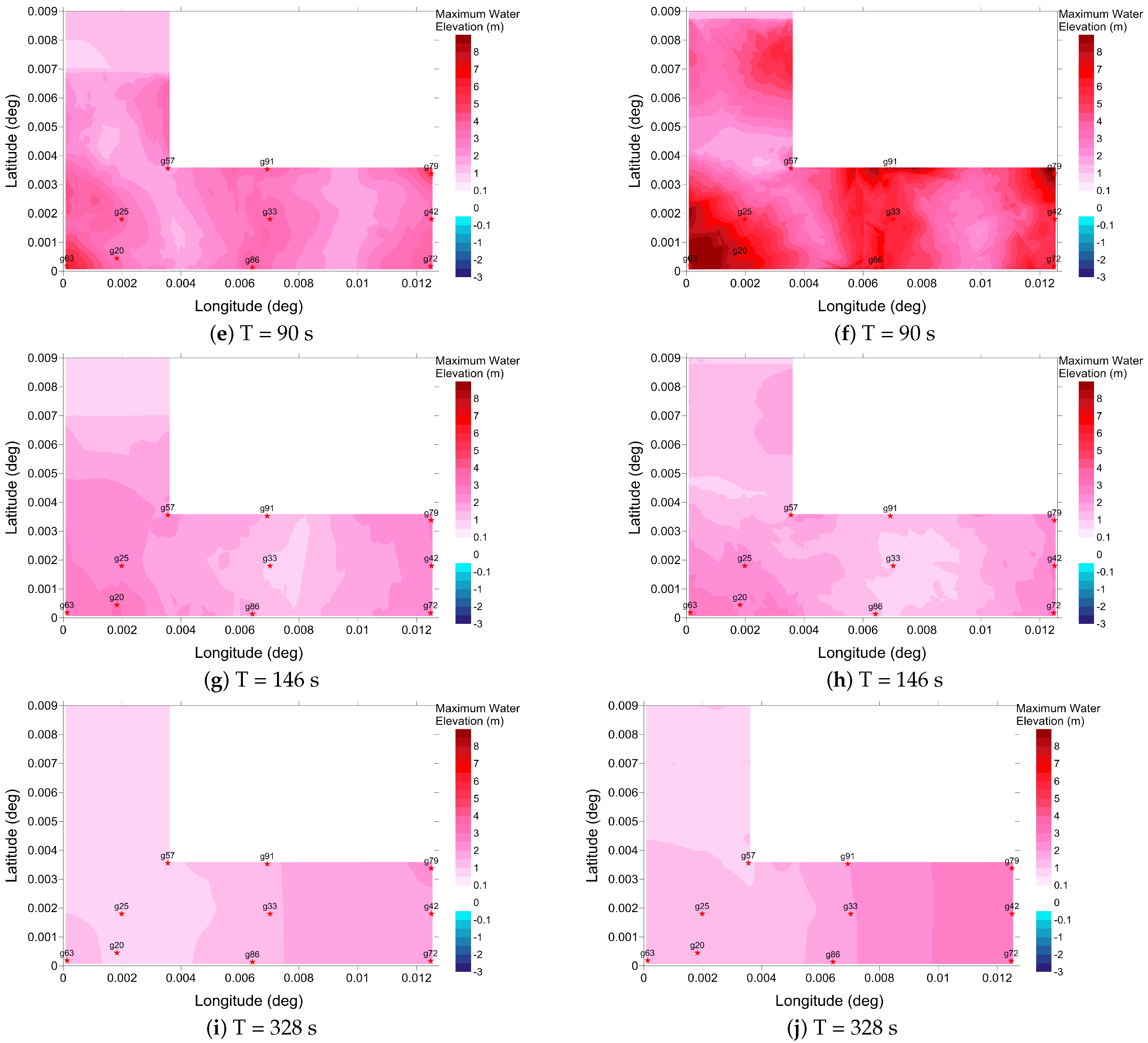
3.1. Free Surface Elevation

The spatial distribution of maximum water elevation, maximum current velocity and the minimum Rouse number are computed at each grid in the domain during the 40-min simulations. Shown in Figure 2 is the maximum water surface elevation for a sinusoidal line crest long wave pertaining to a 1-m wave amplitude LA/LB = 0.8 in the left column and LA/LB = 1 in the right column. The time history of the free surface elevations in two corner points of the basin, Gauge 57 (g57, interior corner) and Gauge 63 (g63, exterior corner), is also shown for the first 30 min in Figure 3.
The results of the maximum water surface elevation in Figure 2 show that the corner points on the bending part of the basin are always the critical points where water surface elevation amplifies in the exterior corner (Gauge 63). Therefore, the time series of free surface elevations are also represented in Figure 3 to evaluate their behavior during the simulation. The seventh mode of the basin free oscillation period (90 s) is a very critical wave period, and there are approximate wave and current amplifications in the entire basin.

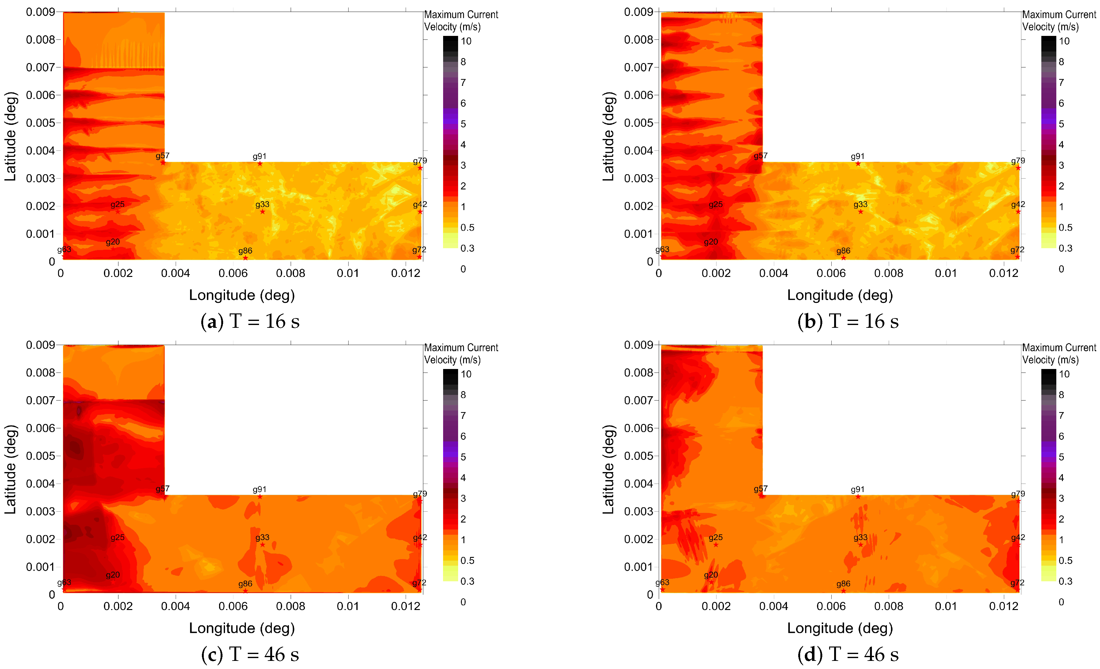
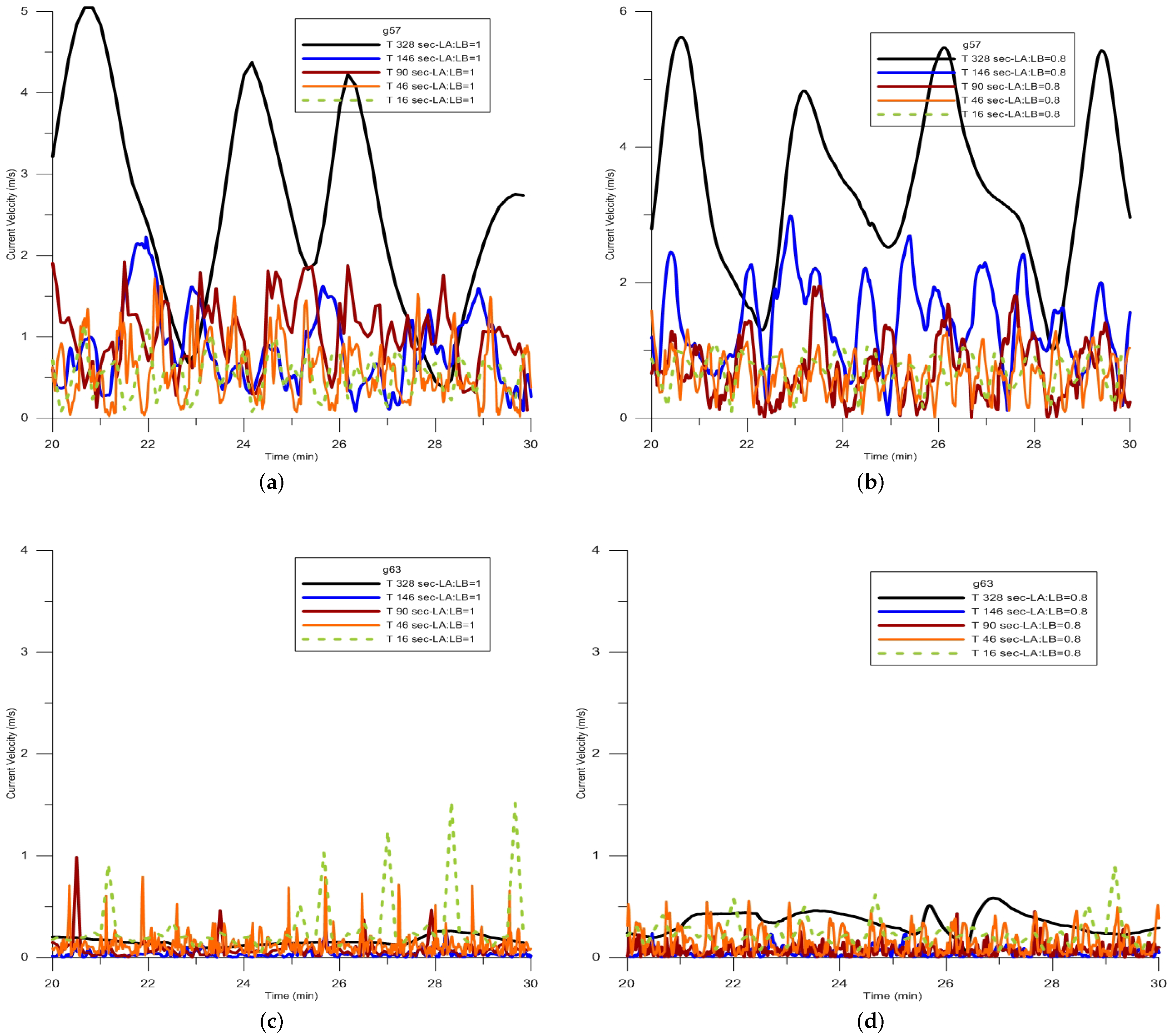
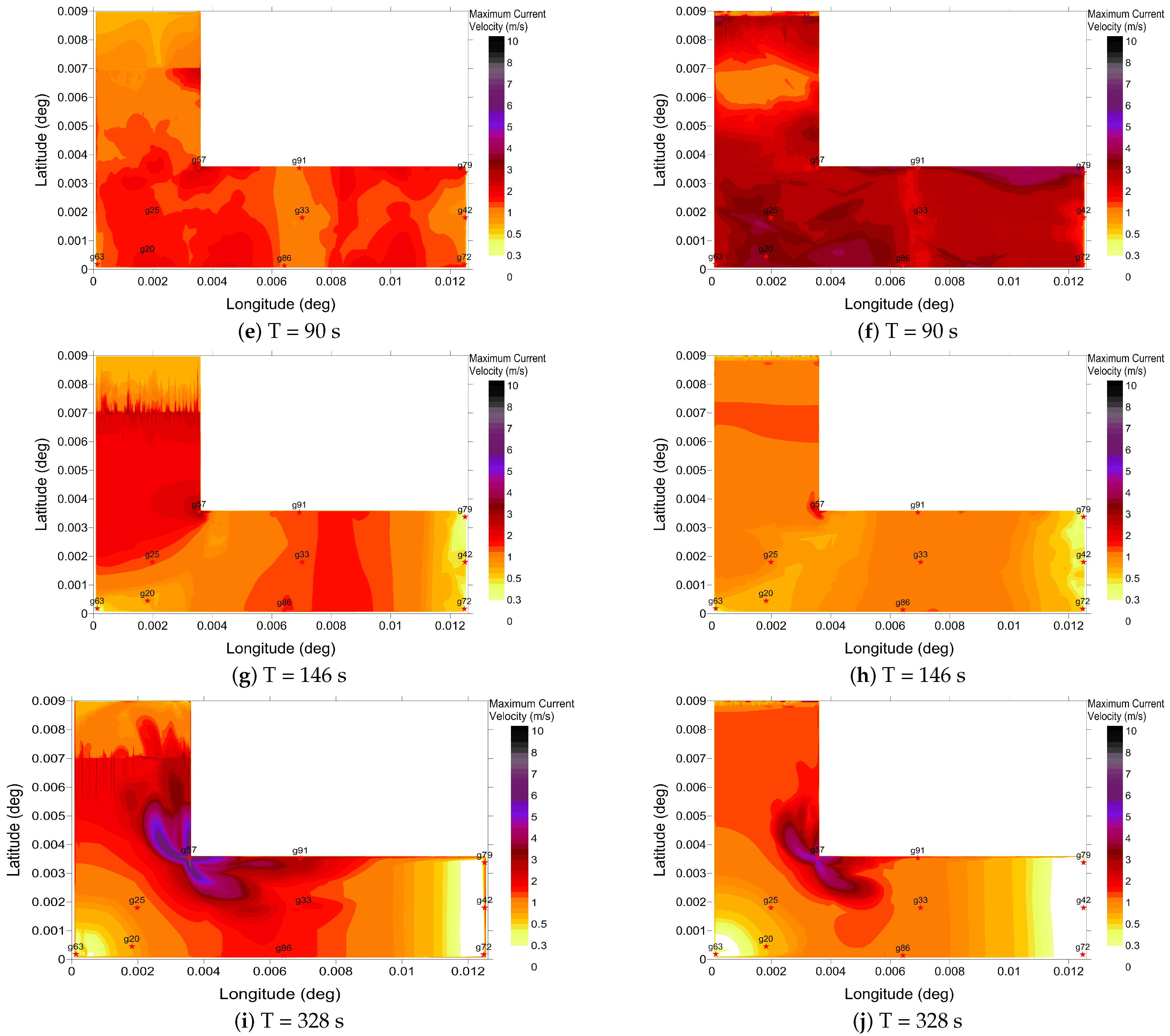
3.2. Current Velocity
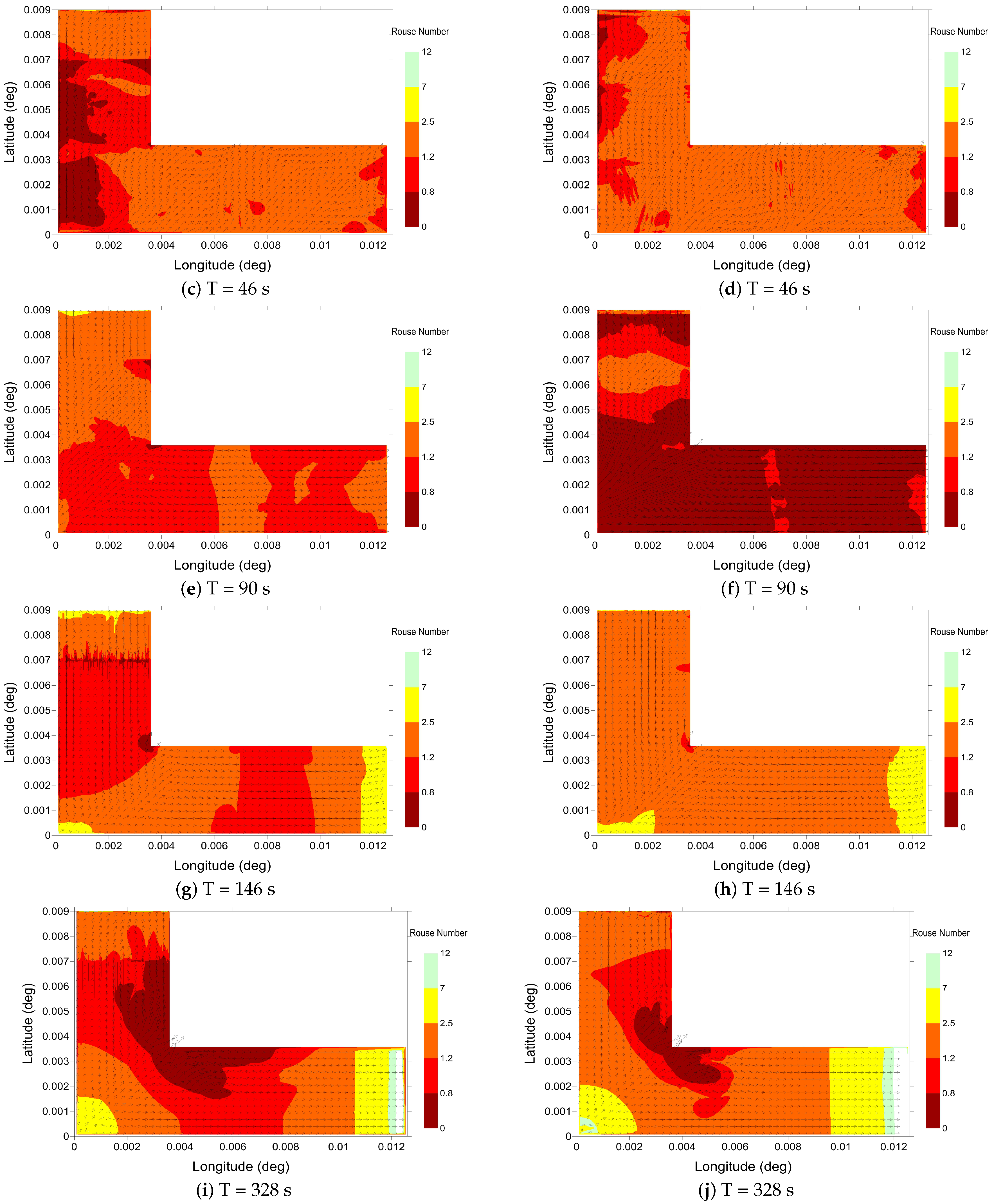
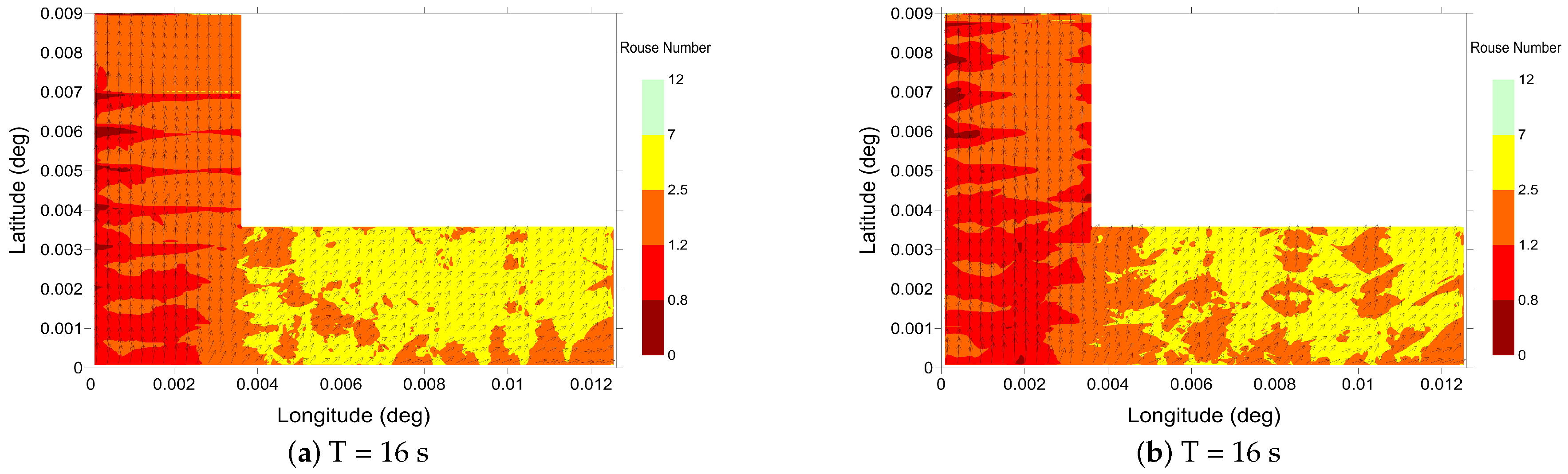
The maximum current velocities for the sinusoidal line crest long wave are shown in Figure 4. The results pertain to a 1-m wave amplitude where the conditions with LA/LB = 0.8 and LA/LB = 1 are depicted in the left and the right columns, respectively. The time history of the current velocity in two corner points of the basin, Gauge 57 and Gauge 63, are shown in Figure 5.
The results presented in Figure 4 demonstrate that the corner points on the bending part of the basin are always the critical points where current velocity amplifies in the interior corners (Gauge 57). Therefore, similar to the previous case, the time series of the current velocity are also represented in Figure 5 to see their behavior during the simulation. Briefly, Gauge 63 in the exterior corner of the L-type basin is the location in which the water surface elevation amplifies extremely, but there is no current amplification. Furthermore, the current velocity amplifies extremely in Gauge 57 in the interior corner of the L-type basin, however with no wave amplification.
Comparing Figure 2 and Figure 4, it can be inferred that in shorter wave periods, the vertical side of the basin (A side) is more exposed to the wave and current amplifications, but in larger wave periods, the maximum values occur in the horizontal side of the L (B side).

3.3. Rouse Number

The minimum Rouse number distribution, as well as the maximum velocity vectors are shown in Figure 6. According to the range of the Rouse number values, the sediment motion in the exterior corner (Gauge 63) is in bed load mode for larger wave periods (T 146 s and 328 s). In the end side of the basin, sediments move in the form of bed load in larger wave periods, as well. This indicates that these areas in the basin have high potential to be exposed by the material deposition.

4. Discussion

The behavior of an L-type basin with a flat depth is studied for wave and current amplification. Furthermore, the sediment motion as a morphological change pattern is investigated via 10 selected gauge points. The results of the maximum water surface elevation, maximum current velocity and minimum Rouse number show that the corner points on the bending side of the basin are always the critical points where water surface elevation and current velocity amplify in the exterior corner point (Gauge 57) and interior corner point (Gauge 63), respectively. Therefore, the time series of free surface elevation and current velocity are also examined to see their behavior during the simulation. According to the time history results of the water surface elevation and current velocity, it is evident that when the vertical side is shorter (LA/LB = 0.8), the amplification magnitude of the free surface elevation and current velocity in the interior corner point of the basin (Gauge 57) is larger than the case with the longer side (LA/LB = 1); however, the opposite holds for the exterior corner point (Gauge 63). Besides, the simulation results show that in the same L-type basin, in shorter wave periods, the wave and current amplifications mostly occur in the vertical side of the basin (A side), where the input source wave begins to propagate. Nevertheless, in larger wave periods, the amplifications take place in the horizontal side of the L-type basin (B side). Therefore, we can conclude that the dimensions of the L-type basin do not affect the occurrence region of the critical points for maximum water surface elevation and maximum current velocity. In all gauge points (except corner points), the wave and current amplify simultaneously if the wave period meets the free oscillation period in the basin. However, it is noticeable that in the interior (smaller) side of L-type basins, the amplification is higher than the exterior (larger) side of it. Furthermore, large periods affect the end parts of the basin more than the smaller wave periods. This phenomenon is more obvious in wave amplification. Comparing the maximum current velocity results with the minimum Rouse number results, one can conclude that the pattern of sediment motion in the mentioned two critical corner points and in the whole basin depends on both the current pattern and magnitude. In large wave periods, the sediment motion in the exterior corner (Gauge 63) is often in the bed load form, while in the interior corner (Gauge 57) in the wash load form. This indicates that, in higher periods, the interior and exterior corners can be exposed to the sediment erosion and deposition, respectively. However, sediment motion in long wave conditions needs further analysis in closed basins, where it becomes a prominent problem for harbors and ports. Further studies on sediment motion seem necessary to determine the performance and validity of NLSWEwhen the volume of the transmitted sediments needs to be measured under the current behavior of the long waves. Furthermore, more investigations should be performed to analyze the behavior of L-type basins with varying depths and then applied to real harbors of this type.

Acknowledgments

Support by 603839 ASTARTE Project of EU, UDAP C-12-14 project of AFAD, Turkey, Russia Turkey Joint Research grant project No. 213M534 of TUBITAK Turkey, grant MK-4315.2015.5 and grants of RFBR 14-05-00092, 15-55-45053 are acknowledged.

Author Contributions

R.K. started with the preliminary simulations and test, developed the necessary database and input wave data, conveyed all simulations, interpreted, compared and discussed the results and prepared the paper. D.V. contributed to the quality and analysis of the data. A.C.Y. and A.Z. took part in the development and insertion of the new module to the numerical tool NAMI DANCE and reviewed the results and discussions.

Conflicts of Interest

The authors declare no conflict of interest.

References

  1. Keshtpoor, M.; Puleo, J.A.; Gebert, J.; Plant, N.G. Numerical simulation of nearshore hydrodynamics and sediment transport downdrift of a tidal inlet. J. Waterw. Port Coast. Ocean Eng. 2014, 141, 0414035. [Google Scholar] [CrossRef]
  2. Keshtpoor, M.; Puleo, J.A.; Shi, F. Downdrift beach erosion adjacent to the Indian River inlet, Delaware, USA. Shore Beach 2014, 82, 31–41. [Google Scholar]
  3. Kian, R.; Yalciner, A.C.; Aytore, B.; Zaytsev, A. Wave amplification and resonance in enclosed basins; A case study in Haydarpasa Port of Istanbul. In Proceedings of the Currents, Waves and Turbulence Measurement (CWTM) 2015 IEEE/OES, St. Petersburg, FL, USA, 2–6 March 2015; Volume 11, pp. 1–7.
  4. Sawaragi, T.; Kubo, M. The motion of a moored ship in a harbour basin. In Coastal Engineering; American Society of Civil Engineers: New York, NY, USA, 1982; pp. 2743–2762. [Google Scholar]
  5. Van der Molen, W.; Monárdez Santander, P.; Van Dongeren, A.R. Modeling of Infragravity Waves and Moored Ship Motions in Tomakomai Port. In Proceedings of the Harbor Long Wave Conference, Yokosuka, Japan, July 2004.
  6. Kioka, W.R. Long period oscillations in a harbour caused by typhoon. In Coastal Engineering; American Society of Civil Engineers: New York, NY, USA, 1996; pp. 1491–1502. [Google Scholar]
  7. Jeong, W.M.; Chae, J.W.; Park, W.S.; Jung, K.T. Field measurements and numerical modelling of harbour oscillations during storm waves. In Coastal Engineering; American Society of Civil Engineers: New York, NY, USA, 1996; pp. 1268–1279. [Google Scholar]
  8. Bellotti, G.; Franco, L. Measurement of long waves at the harbor of Marina di Carrara, Italy. Ocean Dyn. 2011, 61, 2051–2059. [Google Scholar] [CrossRef]
  9. Rabinovich, A.B. Seiches and Harbor Oscillations. In Handbook of Coastal and Ocean Engineering; World Scientific Publishing Co.: Singapore, 2009; pp. 193–236. [Google Scholar]
  10. Thotagamuwage, D.T.P. Harbour Oscillations: Generation and Minimisation of Their Impacts. Ph.D. Dissertation, The University of Western Australia, Perth, Western Australia, 2014. [Google Scholar]
  11. Kakinuma, T.; Toyofuku, T.; Inoue, T. Numerical Analysis of Harbor Oscillation in Harbors of Various Shapes. Available online: https://icce-ojs-tamu.tdl.org/icce/index.php/icce/article/view/6840/pdf (accessed on 1 September 2016).
  12. Kian, R.; Pamuk, A.; Yalciner, A.C.; Zaytsev, A. Effects of tsunami parameters on the sedimentation. In Proceedings of the Coastal Sediments Conference (CS15), San Diego, CA, USA, 13–15 May 2015; Volume 8, pp. 67–74.
  13. Yeh, H.; Li, W. Tsunami scour and sedimentation. In Proceedings of the 4nd International Conference on Scour and Erosion, American Geophysical Union, San Francisco, CA, USA, December 2008; pp. 95–106.
  14. Zaytsev, C.; Yalciner, P.K. (Eds.) Tsunami Simulation/Visualization Code NAMI DANCE versions 4.9. NAMI DANCE Manual. 2010. Available online: http://www.namidance.ce.metu.edu.tr (accessed on 3 July 2014).
  15. Ergin, M.; Keskin, S.; Dogan, A.U.; Kadıoglu, Y.K.; Karakas, Z. Grain size and heavy mineral distribution as related to hinterland and environmental conditions for modern beach sediments from the Gulfs of Antalya and Finike, eastern Mediterranean. Mar Geol. 2007, 240, 185–196. [Google Scholar] [CrossRef]
  16. Pamuk, A. Assessment of Inland Tsunami Parameters and Their Effects on Morphology. Master's Thesis, Middle East Technical University, Ankara, Turkey, 2014. [Google Scholar]
  17. Kian, R. Tsunami Induced Wave and Current Amplification and Sedimentation in Closed Basins. Ph.D. Dissertation, Middle East Technical University, Ankara, Turkey, 2015. [Google Scholar]
Figure 1. L-type basin used in the simulations. (a) LA is the vertical dimension and LB the horizontal dimension of the L-type basin. (b) Dimensions are in the geographical outline. Red stars represent the gauge points.
Jmse 04 00055 g001
Figure 2. The spatial distribution of the maximum water surface elevation (m) computed by the simulation of the sinusoidal line crest long wave with a 1-m wave amplitude with T = 16 s, T = 46 s, T = 90 s, T = 146 s, T = 328 s for LA/LB = 0.8 in the left column and LA/LB = 1 in the right column.
Jmse 04 00055 g002aJmse 04 00055 g002b
Figure 3. Time history of water surface elevation computed by the simulation of the sinusoidal line crest long wave with a 1-m wave amplitude with T = 16 s, T = 46 s, T = 90 s, T = 146 s, T = 328 s for LA/LB = 1 (left column), for LA/LB = 0.8 (right column) in Gauge 57 (a,b) and Gauge 63 (c,d).
Jmse 04 00055 g003
Figure 4. The spatial distribution of the maximum current velocity (m/s) computed by the simulation of the sinusoidal line crest long wave with a 1-m wave amplitude with T = 16 s, T = 46 s, T = 90 s, T = 146 s, T = 328 s for LA/LB = 0.8 in the left column and LA/LB = 1 in the right column (aj).
Jmse 04 00055 g004aJmse 04 00055 g004b
Figure 5. Time history of the current velocity computed by the simulation of the sinusoidal line crest long wave with a 1-m wave amplitude with T = 16 s, T = 46 s, T = 90 s, T = 146 s, T = 328 s for LA/LB = 1 (left column), for LA/LB = 0.8 (right column) in Gauge 57 (a,b) and Gauge 63 (c,d).
Jmse 04 00055 g005
Figure 6. The spatial distribution of the minimum Rouse number computed by the simulation of the sinusoidal line crest long wave with a 1-m wave amplitude with T = 16 s, T = 46 s, T = 90 s, T = 146 s, T = 328 s for LA/LB = 0.8 in the left column and LA/LB = 1 in the right column (aj), respectively. The maximum velocity vectors are also shown for each case.
Jmse 04 00055 g006aJmse 04 00055 g006b
Table 1. Typical constants.
ν, Kinematic Viscosity 1.0 × 10 - 6   m 2 /s
g, Gravitational Acceleration 9.81 m/ s 2
ρ, Density of Water1025 kg/ m 3
ρ s , Density of Sediment Particles2650 kg/ m 3
Table 2. Modes of transport according to the Rouse number [13].
Mode of TransportRouse Number
Initiation of Motion (Deposition) R 0 > 7
Bed Load 2.5 < R 0 < 7.5
Suspended Load: (50% Suspended), Density of Water 1.2 < R 0 < 2.5
Suspended Load: (100% Suspended) 0.8 < R 0 < 1.2
Wash Load R 0 < 0.8

