An Open-Access, Multi-Decadal, Three-Dimensional, Hydrodynamic Hindcast Dataset for the Long Island Sound and New York/New Jersey Harbor Estuaries

Abstract

This article presents the results and validation of a comprehensive, multi-decadal, hindcast simulation performed using the New York Harbor Observing and Prediction System´s (NYHOPS) three-dimensional hydrodynamic model. Meteorological forcing was based on three-hourly gridded data from the North American Regional Reanalysis of the US National Centers for Environmental Prediction. Distributed hydrologic forcing was based on daily United States Geologic Survey records. Offshore boundary conditions for NYHOPS at the Mid-Atlantic Bight shelf break included hourly subtidal water levels from a larger-scale model ran for the same period, tides, and temperature and salinity profiles based on the Simple Ocean Data Assimilation datasets. The NYHOPS model’s application to hindcast total water level and 3D water temperature and salinity conditions in its region over three decades was validated against observations from multiple agencies. Average indices of agreement were: 0.93 for storm surge (9 cm RMSE, 90% of errors less than 15 cm), 0.99 for water temperature (1.1 °C RMSE, 99% of errors less than 3 °C), and 0.86 for salinity (1.8 psu RMSE, 96% of errors less than 3.5 psu). The model’s skill in simulating bottom water temperature, validated against historic data from the Long Island Sound bottom trawl survey, did not drift over the years, a significant and encouraging finding for multi-decadal model applications used to identify climatic trends, such as the warming presented here. However, the validation reveals residual biases in some areas such as small tributaries that receive urban discharges from the NYC drainage network. With regard to the validation of storm surge at coastal stations, both the considerable strengths and remaining limitations of the use of North American Regional Reanalysis (NARR) to force such a model application are discussed.

1. Introduction

Every year since 1976 has had an average global temperature warmer than the long-term average. Over the 1979–2013 period, global temperature warmed at an average of 0.26 °C per decade over land and 0.10 °C per decade over the global ocean [1]. The recently signed Paris Agreement [2], adopted by 195 countries, has a long-term goal of keeping the increase in global average temperature to well below 2 °C above pre-industrial levels, and aims to limit the increase to 1.5 °C, as doing so is expected to significantly reduce risks and the impacts of climate change. Yet, the Northeast US shelf waters have experienced higher warming rates than the global ocean, deduced by the Sea Surface Temperature (SST) satellite record. Pershing et al. [3] reported that SST rose by 0.30 °C per decade between 1982 and 2013 in the Gulf of Maine. The sole long-term observation record for water temperatures within the Long Island Sound (LIS) estuary, a US Estuary of National Significance, at a location near Millstone CT [4] has measured a much more rapid increase in LIS water temperatures than the global average: an alarming 0.44 °C per decade between 1979 and 2013, over four times higher than the global average rate. Over coastal Connecticut counties, on LIS’s northern coast, surface air temperatures for the same time period increased by 0.33 °C per decade; that rate was double if only the 1992–2012 period was considered, but has decreased somewhat since, to 0.28 °C per decade (1979–2015; [1]).

Over these last few decades, the LIS ecosystem has undergone profound changes. Ocean warming is suggested to be the most important factor associated with the observed shifts in the mean center of biomass in Northeast U.S. fisheries [3,5,6,7]. However, understanding what controls the observed trends in the Northeast U.S., and how such processes affect the LIS ecosystem, has been limited due to the paucity of available three-dimensional, physical data. In 2013, the New York and Connecticut Sea Grants and the US EPA Long Island Sound Study joined forces to fund a multi-disciplinary project to address this deficiency, spearheading collaborative research involving numerical modelers, climate scientists, and fishery biologists. The work evaluated conditions and identified warming, freshening, and estuarine circulation trends in Long Island Sound over the past three decades. This research also explored how global climate contributes to long-term and inter-annual variability in the LIS physical environment and its Living Marine Resources [8].

This research article, presented at the 14th Estuarine and Coastal Modeling Conference (ECM14, http://ecm.github.io/ECM14/), focuses on the validation and results of a comprehensive, multi-decadal, hindcast simulation performed using the New York Harbor Observing and Prediction System (NYHOPS) hydrodynamic model that generated a continuous, three-dimensional dataset for a coastal aquatic region that includes Long Island Sound and the New York/New Jersey Harbor (NYNJH) Estuaries, between 1981 and 2013. Section 2 describes the data and methods used to set up the multi-decadal hindcast and the data and methods used to validate it for LIS and NYNJH and to have it serve as an open access dataset. Section 3 presents validation results. Section 4 puts the importance of the validation in perspective and discusses identified or verified trends and climatologies based on the validated model. Conclusions are outlined in the last section. Supplementary material in the form of a comprehensive PowerPoint presentation configured in two parts is also provided.

An online THREDDS Data Server (http://colossus.dl.stevens-tech.edu/thredds/catalog.html) was set up to serve the NYHOPS model’s results in oceanographic NetCDF format over the web using the OPENDAP protocol, enabling open access to daily averaged or monthly averaged time series for all the gridded hindcast physical variables in or over the NYHOPS region (including LIS and NYNJH). Simulated climatologies (mean simulated climate conditions averaged over the three decades of the NYHOPS hindcast period) for two- and three-dimensional fields such as water temperatures and salinities, were also generated, and included in THREDDS. The use of the validated results of the model to research global climate teleconnections to the LIS ecosystem and its living marine resources will be presented in subsequent papers that are presently under preparation.

2. Materials and Methods

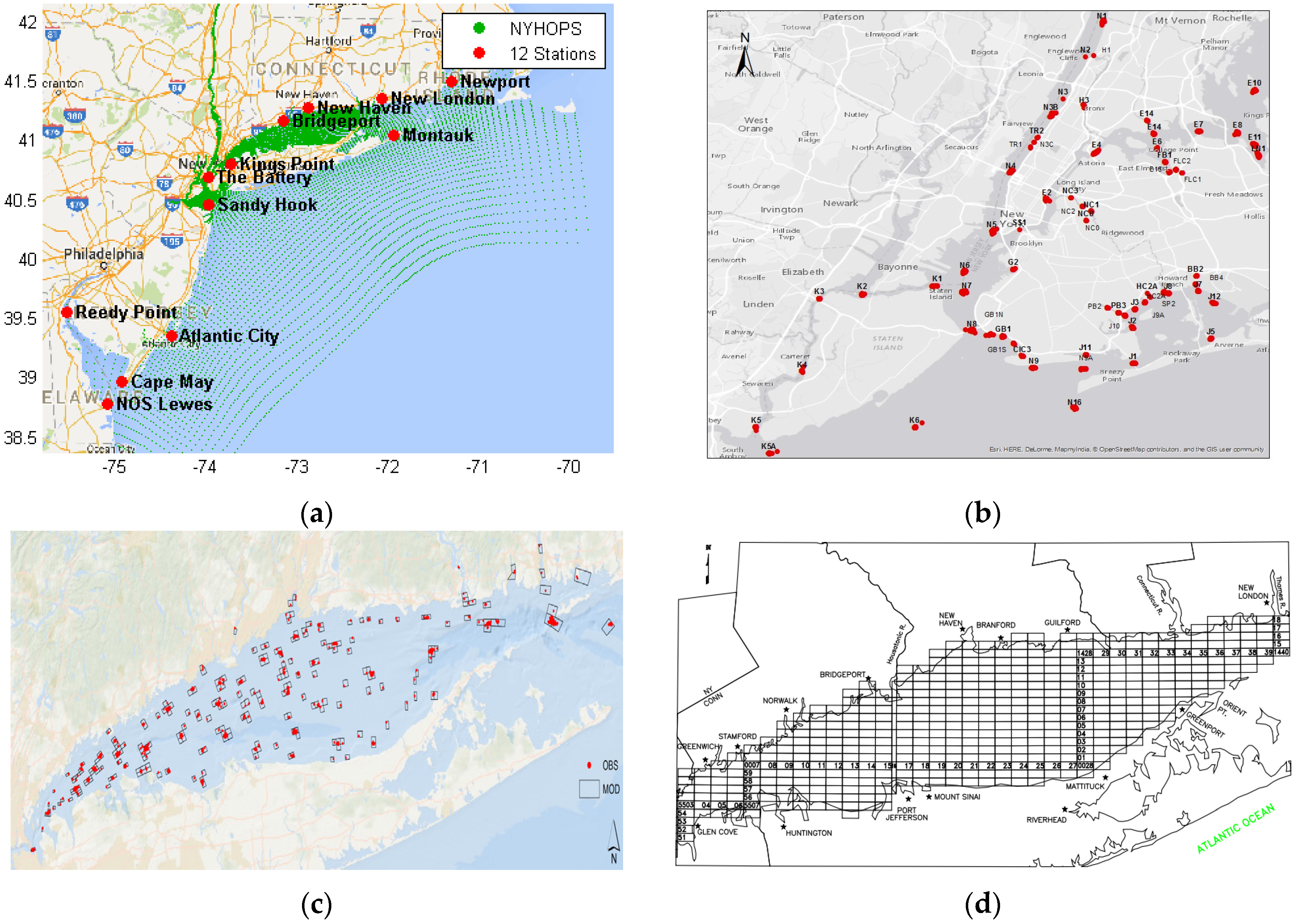
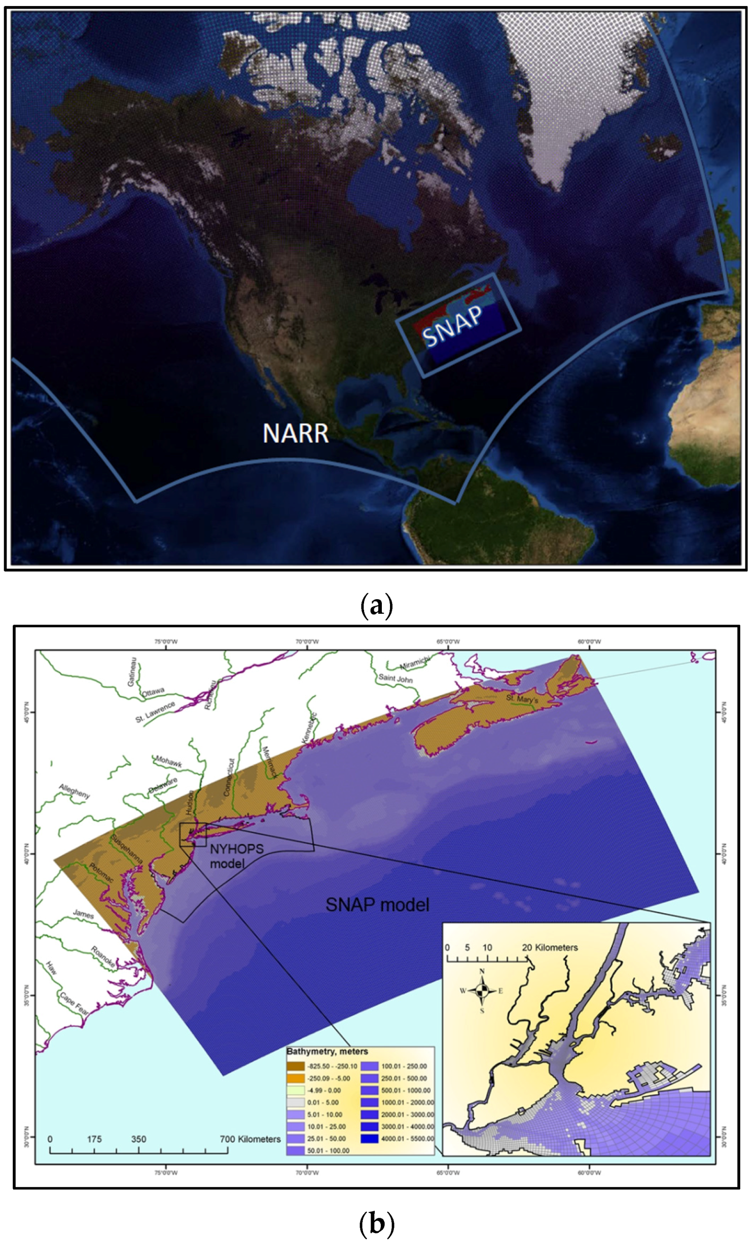
The completed multi-decadal high-resolution three-dimensional hindcast simulation for LIS and NYNJH was based on a nested modeling concept utilizing two hydrodynamic domains (Figure 1): The Stevens North Atlantic Predictions model (SNAP) [9,10,11] and the New York Harbor Observing and Prediction System model (NYHOPS, www.stevens.edu/NYHOPS) [9,11,12,13,14,15,16,17,18]. Both domains were simulated in 3D with the Stevens Estuarine and Coastal Ocean Model code (sECOM) [11,14,19], a derivative of the Princeton Ocean Model [20]. The SNAP model was run first, in a diagnostic mode (clamping temperature and salinity at the initial condition), at its regular 5 km resolution grid for the complete 1979–2013 simulation. SNAP wave and water level results, along with observation-based temperature and salinity fields, were then used to derive NYHOPS offshore boundary conditions and force the NYHOPS prognostic hindcast simulation on its variable-resolution grid (4 km to 25 m horizontal resolution, 10 vertical sigma layers). This is the same nesting concept used operationally for the ensemble-based Stevens Flood Advisory System (www.stevens.edu/SFAS [11]).

Surface meteorological forcing to both SNAP and NYHOPS was based on gridded data from the North American Regional Reanalysis (NARR [21]) created for the US National Centers for Environmental Prediction (NCEP). NARR (Figure 1) has been shown to have good skill for regional climate studies [22], but may be deficient for strong Atlantic precipitation events and Atlantic hurricanes [21]. Three-hourly surface meteorological variables provided by NARR at its 32 km grid were interpolated to the SNAP and NYHOPS grids and used to force the two models throughout the hindcast. Winds at 10 m above surface and barometric pressure reduced to mean sea level, total cloud cover, relative humidity and air temperature at 2 m above ground were used to compute locally dynamic surface heat flux terms, surface stress terms and surface wave growth terms with the methodology described in [14] and [23] as progressed by Orton et al. [17] based on internally calculated surface wave fields and explicit wave-steepness by Taylor and Yelland [24].

In the construction of the three dimensional NYHOPS hindcast, great care was put into creating high-fidelity lateral and internal boundary conditions for hydrodynamic forces included in the NYHOPS model, to complement the surface meteorological forcing provided by NARR. SNAP model results were used to provide hourly offshore boundary conditions to NYHOPS at the Mid-Atlantic Bight shelf break for surface waves and offshore tidal residuals (storm surge), the latter being used to provide the subtidal part to the tidal NYHOPS water level boundary conditions as in [14,15]. An attempt was made to account for steric and mean sea level rates across the NYHOPS simulations by adding the spatially and-seasonally averaged residual errors across SNAP coastal station predictions within the NYHOPS domain to the NYHOPS offshore water level boundary conditions [14,15]; average rates are listed in [25]. The observed water level records used in this step were tied to the geodetic NAVD88 datum.

Further, to provide offshore temperature and salinity profiles at the continental shelf break to NYHOPS for the hindcast, monthly data from the Simple Ocean Data Assimilation (SODA) climatology for water temperature (T) and salinity (S) were acquired beginning in 1959 on a global 0.5 degree geographic resolution grid with 40 standard depth levels in the vertical [26]. Some issues were identified with the continuity and versioning of the available SODA datasets that required significant effort in order to create a consistent monthly climatological dataset for the complete NYHOPS hindcast period of 1979–2013. A unified set of NYHOPS boundary conditions was created using SODA version 2.1.6 from 1979–1999, then SODA version 2.2.4 from 2000–2010, then results from a ROMS model run [18] generated at Rutgers University nested within a global HYCOM model for 2011–2012, and finally HYCOM global model results for 2013 [27]. To decrease climatologically relevant discrepancies between the last two datasets and SODA, bias correction for the last two datasets was performed both for the T/S means and their range. The native ROMS results for 2011–2012 were bias-corrected based on mean and range anomalies between the SODA version 2.2.4 datasets and the ROMS-with-HYCOM datasets for the common years of 2005–2008. HYCOM for 2013 was similarly bias-corrected based on the same debiasing factors. The assumption was that if the ROMS and HYCOM models were biased compared to SODA years 2005–2008 (shifted and inflated/deflated), they would continue being biased in a similar fashion in subsequent years. This assumption was validated by comparing the debiased datasets against SODA 2.2.4 for the last two SODA years, 2009–2010. Both means and ranges were significantly closer to SODA after debiasing (not shown). After the unified monthly T/S dataset from 1979 to 2013 was created at SODA resolution, it was interpolated in space and time along the NYHOPS offshore boundary, checked for vertical density stability, and used to force the NYHOPS 3D hindcast simulation.

Distributed hydrologic forcing to the NYHOPS estuarine model was based on daily United States Geologic Survey (USGS) records [25] with comparable but expanded results to other regional published studies [28,29]. 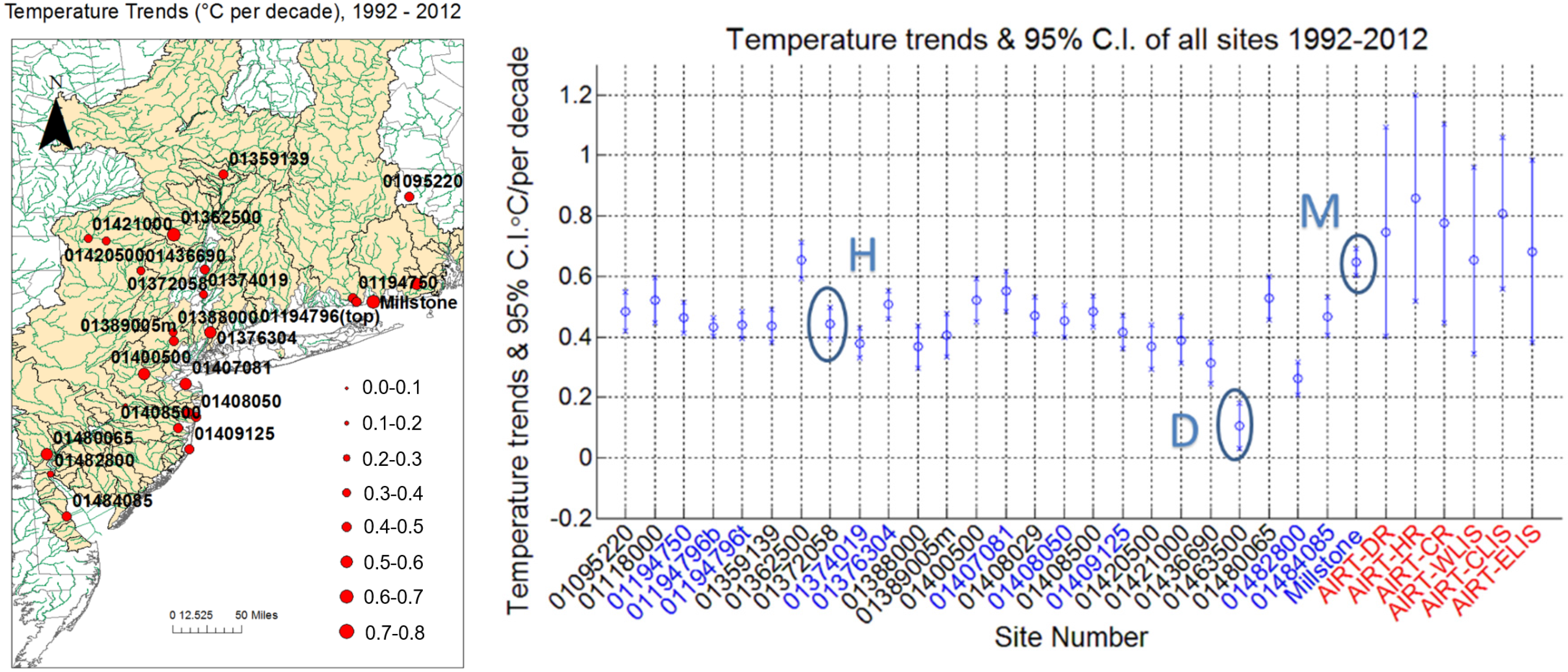As part of this work, a fluvial temperature study for rivers with long temperature time series across the Mid-Atlantic was completed to aid with the assignment of daily temperatures to riverine discharges in the NYHOPS hindcast (NYHOPS includes an extensive hydrologic input network [14]). That work was presented at the annual Mid-Atlantic Bight Oceanography and Meteorology Meeting (MABPOM 2013). Results indicated that river temperatures, and associated thermal inputs to Mid-Atlantic waters increased—similarly to, though somewhat less rapidly than, the regional air temperature trends—with variation in the positive rate values between different MAB watersheds (Figure 2). River flows also increased considering the 1979–2013 period as a whole. Based on linear trends estimated from the USGS discharge data, major freshwater river inflow rates to the LIS and NYNJH increased significantly: the Connecticut River at Thompsonville (USGS station ID 01184000) by 17%—the Connecticut River contributes about 75% of total freshwater flow into LIS—the Housatonic River at Stevenson (USGS station ID 01205500) by 21%, and the Hudson River at Green Island by 33% (USGS station ID 01358000). The completed daily time series of estimated river flows and temperatures from 1979 to 2013 were used as distributed discharge forcing in the NYHOPS 3D hindcast. Ungauged tributaries in NYHOPS are included through basin-area scaling of observed hydrographs from proximal gauged rivers. Finally, distributed end-of-pipe Point Source forcing is also included in NYHOPS model runs based on monthly climatologies of waste water treatment plant effluent and power plant intake/outfall pairs [14].

The model hindcast simulation period started in 1979 and completed in 2013. The first two years were considered spin-up years for 3D hydrodynamics. Therefore, for consistency, results will be presented from 1981 on. This hypothesis was tested in LIS by considering different initial conditions updated every five years from the hindcast. It was found that the NYHOPS solution for T and S within the LIS estuary would converge well within two years from initiation.

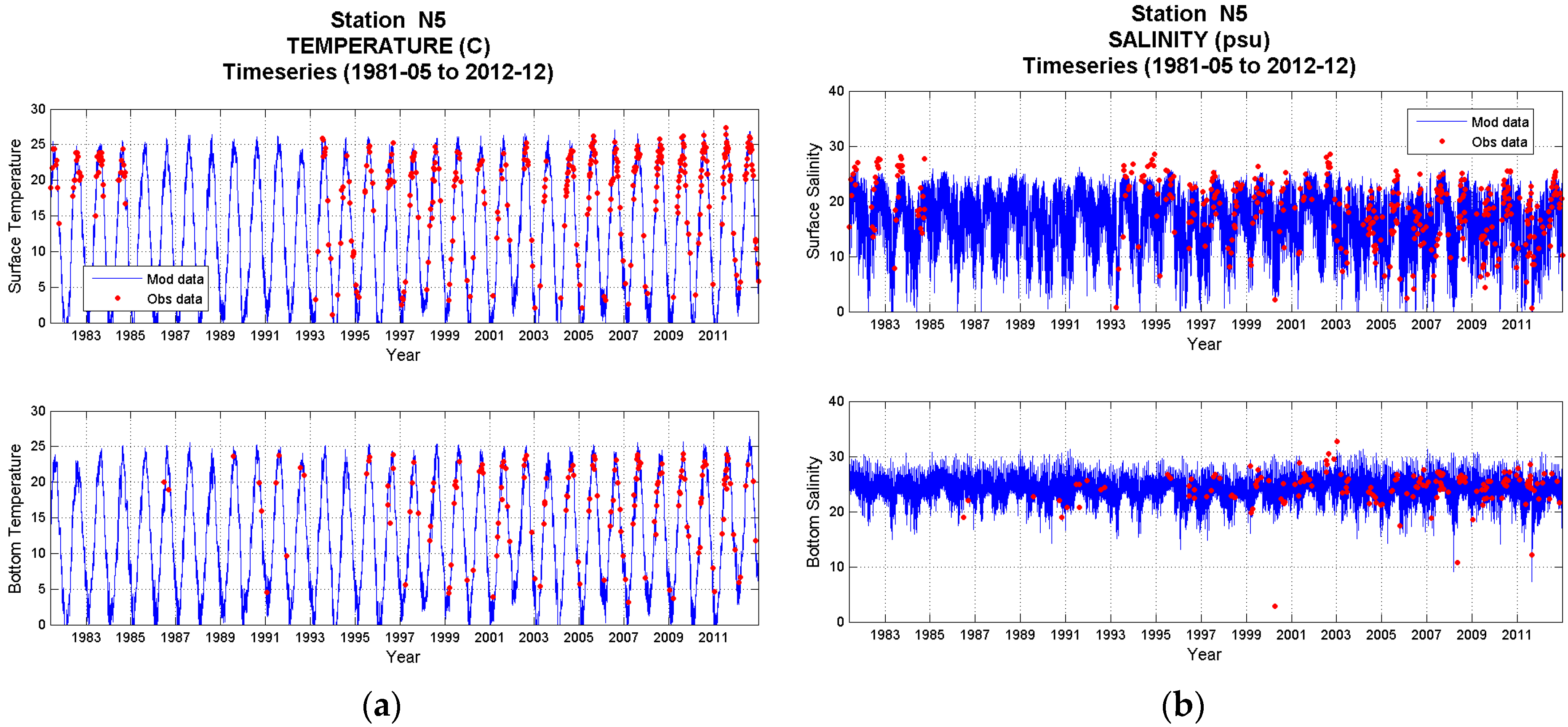
The NYHOPS model’s application to hindcast total water level, and 3D water temperature and salinity conditions in its region over three decades was validated extensively against various available observational datasets. Hourly total water levels collected by the National Ocean Service (NOS) at 12 coastal stations within the NYHOPS domain between 1979 and 2013 were used to quantify the model’s performance to storm surge after subtraction of the NOS-predicted astronomical tide (Figure 3a). 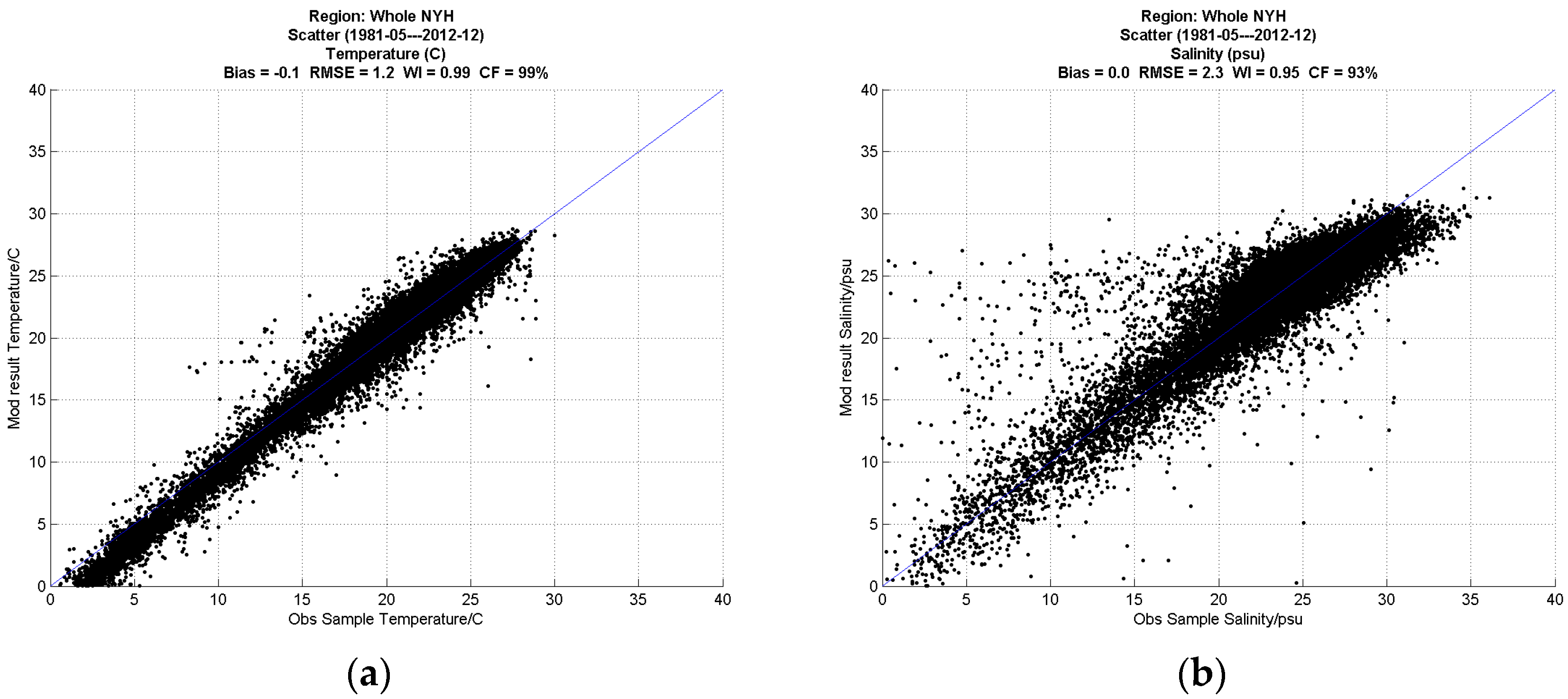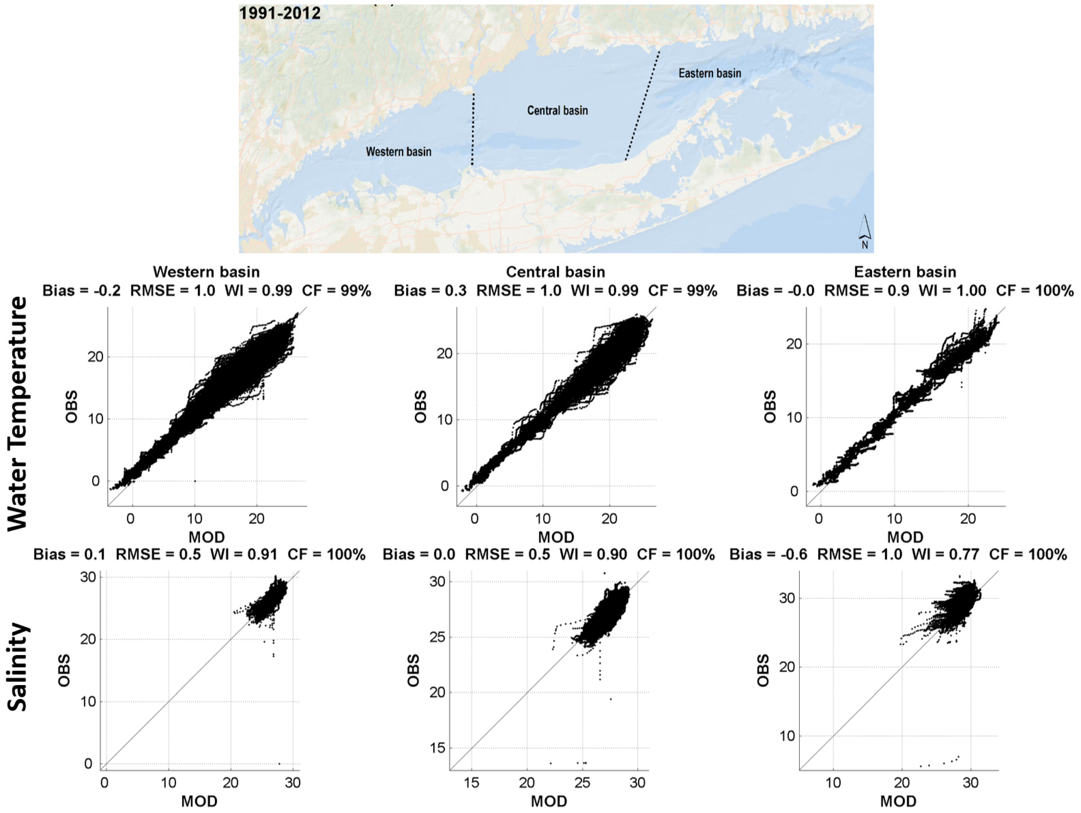Near-surface and near-bottom T and S grab samples taken with variable frequency—weekly to biweekly, and mostly during summer—from a New York City Department of Environmental Protection (NYC DEP) boat between 1981 and 2012 were used to quantify the skill of the model for T and S at NYC DEP stations in NYNJH (Figure 3b). Vertical CTD casts from cruise surveys conducted for the Long Island Sound Study between 1991 and 2012 as provided by the Connecticut Department of Energy and Environmental Protection (CT DEEP) were used to quantify the skill of the model for T and S in LIS (Figure 3c). Near-bottom temperatures collected on a regular grid that covers most of the LIS bottom by CT DEEP fisheries as part of the Long Island Sound Trawl Survey between 1992 and 2013 were used to test whether the model’s skill in simulating bottom water temperature showed signs of drift over the years in LIS (Figure 3d). Finally, an observations-based monthly three-dimensional temperature and salinity climatology dataset called MOCHA version-2 created at Rutgers University in New Jersey (http://tds.marine.rutgers.edu/thredds/catalog/other/climatology/mocha/catalog.html; [30] as updated in MOCHA’s 2nd version in 2012) was used to quantify the skill of the NYHOPS hydrodynamic model for T and S against climatology. MOCHA is a three-dimensional climatological analysis of the temperature and salinity, with a 0.05 degree (~5 km) grid in the horizontal and 55 standard depths in the vertical that covers the MAB, from 45° N to 32° N, 77° W to 64° W. It is derived from all in situ data available from the NODC World Ocean Database 2005 and the NOAA North East Fisheries Science Center database. Comparisons to MOCHA were only made in LIS as the NYNJH is not well resolved in its grid.

Adopting NOS guidelines and prior literature used for validating the operational NYHOPS forecast model [11,15,16,31], the following metrics were used to quantify model skill in the Results section:

• Bias or mean error, M.E.: The mean error between model and observations.
• RMSE: The square root of the average error between model and observations squared.
• R-square, R²: The square of the correlation coefficient between model and observations.
• Willmott Skill or Index of Agreement, W.I. [32]: A non-dimensional measure of how close the model’s results are to observations. Values are between 0 and 1, with 1 being a perfect “skill score.”
• Central frequency of error, C.F.: The percent of errors that are below a given threshold that is considered high for operational use. The larger the C.F., the better the model. NOS usually considers a C.F. ≥ 90% as accepted model performance against the following thresholds: 15 cm for total water level, 3.0 °C for T, and 3.5 psu for S [31].
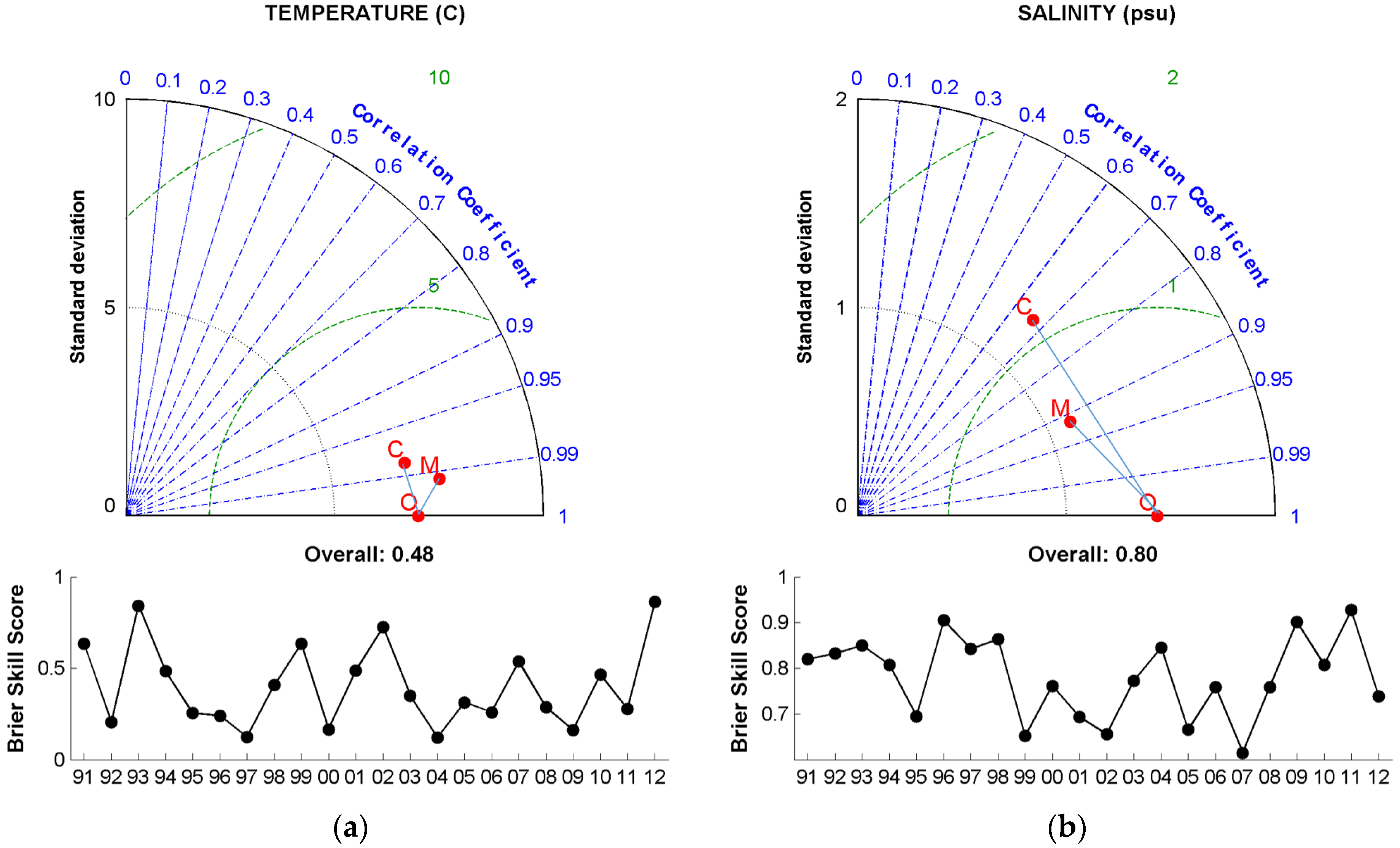
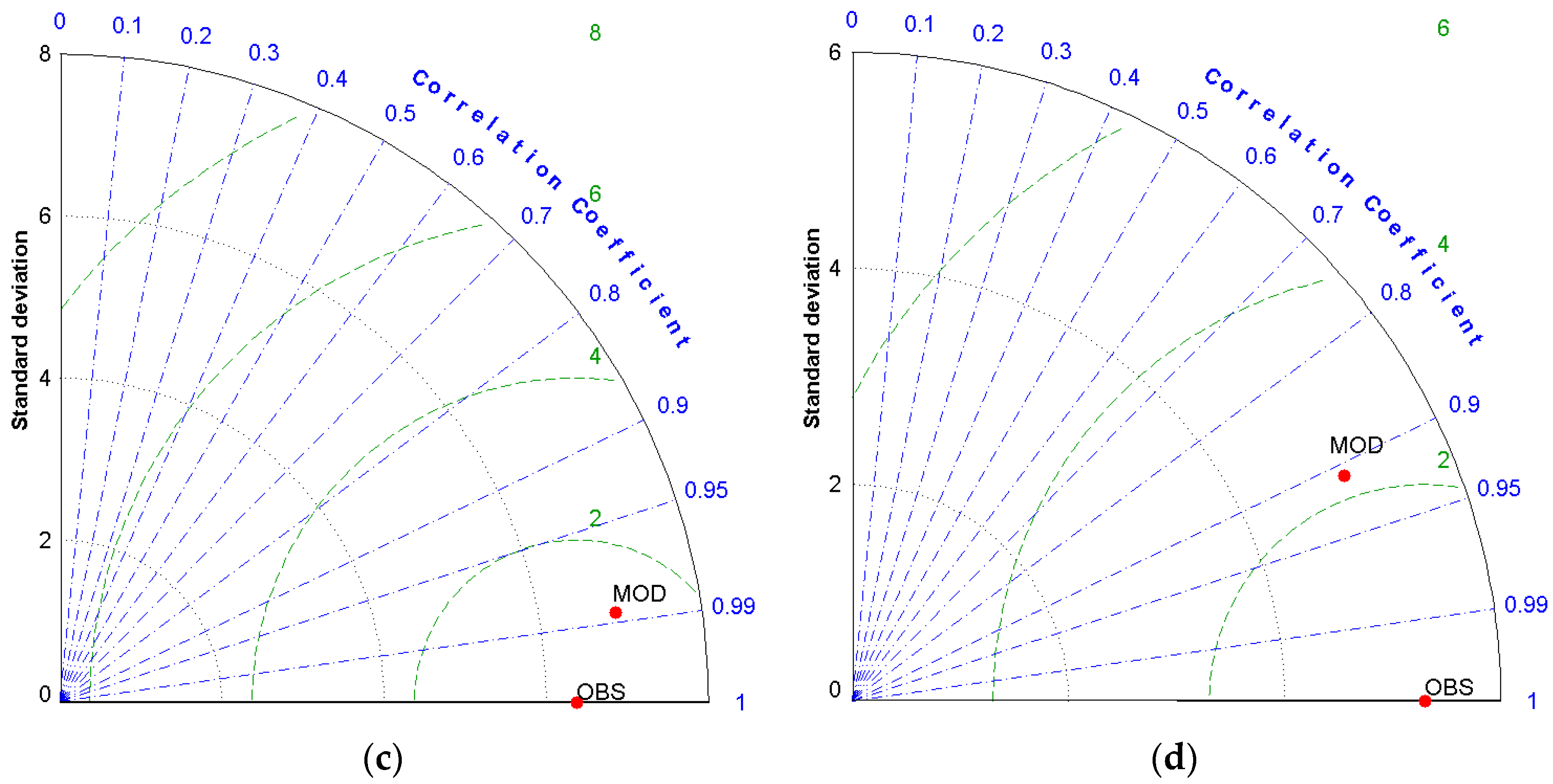
• Taylor diagram, [33]. The Taylor Diagram provides a visual statistical summary of how well the model and observation patterns match each other in terms of their correlation coefficient (R), their root mean square error (RMSE), and their standard deviation (σ).
• Brier Skill Score, B.S.S. [34]: The Brier Skill Score essentially compares the magnitude of the difference between a model (NYHOPS here) and observations to that achieved by a reference model (the monthly MOCHA climatology here). The B.S.S. is written as

  $$BSS=1‒\frac{1}{N_i}\sum _{j=1}^{N_i}{(d_{i,j}‒p_{i,j})}^2/\frac{1}{N_i}\sum _{j=1}^{N_i}{(d_{i,j}‒r_{i,j})}^2$$

  (1)

where the vector d_i,j contains the j = 1, 2,…, N_j measurements (in situ observations). Similarly, p_i,j are the model predictions at the same time and location of the data, d_i,j, and the vector r_i,j contains the predictions of the reference climatology (MOCHA here). BSS compares the ratio of the variance in the observations not explained by the model to that not explained by the reference climatology. If BSS > 0, then the model is in better agreement with the data than the reference model. Conversely, if BSS < 0, it is not as good.

NYHOPS model results were interpolated from the native NYHOPS grid to the location and time of individual observations, before making comparisons. It is important to note that there are always discrepancies in the observations due not only to the precision of the instruments and analyses methods, but also due to the difference in the property simulated (the average over a model cell’s volume and output time step) and that measured (sometimes a few samples from a bottle). Even a perfect model, therefore, should not be expected to have BSS = 1, (nor will W.I. and R² be equal to unity for that matter). Given however the comparison to average climatology, BSS for a skillful model should be consistently higher than 0, and hopefully closer to unity. Finally, binned histograms of model errors against observations were also used to show uncertainty in model results, and whether that uncertainty grew or decreased over the hindcast years.

3. Results

The model’s grand-mean temperature and salinity bias against all Long Island Sound Study observations in the Sound was found to be 0.18 °C warmer for water temperature, and 1.31 psu saltier for salinity; these biases were assumed constant in time and space and were removed from all raw NYHOPS model gridded time series results. The local tidal correction procedure described in [16] was applied to the raw NYHOPS water level results for the 12 coastal stations. The astronomical tide predicted by NOS at these stations was used in that correction, and then removed from the total water level signals to calculate storm surge. The results used and shown below are after these treatments were put into effect.

3.1. Storm Surge Validation

Figure 4 shows example storm surge results at The Battery, NY, highlighting the storm surge validation that was performed at each of the 12 NOS stations. The highest storm surge (SS) and total water level (TWL) values at The Battery for the 1981–2013 time period shown were simulated by NYHOPS to have occurred during Hurricane Sandy in 2012. Although this is consistent with the observed record, the NARR-forced NYHOPS hindcast under-predicted surge during that storm by about 2 feet or ~20%.

Table 1. NYHOPS hindcast performance metrics for total water level (TWL) and storm surge (SS) at 12 NOS stations.

Station Name	Dates	RMSE, cm	CF ≤ 15 cm, %	R2SS	R2TWL	WISS
Lewes, DE	1979–2012	8.6	91.9	0.78	0.97	0.94
Reedy Point, DE	1996–2013	14.1	71.7	0.63	0.96	0.88
Cape May, NJ	1979–2013	7.8	94.6	0.80	0.98	0.95
Atlantic City, NJ	1985–2013	6.6	97.2	0.86	0.98	0.96
Sandy Hook, NJ	1979–2013	9.0	91.1	0.76	0.97	0.93
The Battery, NY	1979–2013	9.3	89.9	0.74	0.97	0.93
Kings Point, CT	1998–2013	12.8	76.4	0.65	0.99	0.90
Bridgeport, CT	1996–2013	11.6	79.8	0.65	0.98	0.89
New Haven, CT	1999–2013	9.1	90.6	0.75	0.99	0.93
Montauk, NY	1979–2013	5.7	98.9	0.85	0.95	0.96
New London, CT	1979–2013	7.1	96.5	0.78	0.96	0.94
Newport, RI	1979–2013	7.4	95.6	0.72	0.97	0.92

lists NYHOPS hindcast performance metrics for TWL and SS using the methods of Georgas and Blumberg [15] against NOS observations at 12 coastal stations. RMSE varied between 5.7 cm at Montauk, NY and 14.1 cm at Reedy Point, DE, the latter being in a region (Delaware Bay) not well resolved by the NYHOPS model’s horizontal grid. R² for TWL that includes astronomical tide varied between 0.95 at Montauk and 0.99 at New Haven, Kings Point, and Bridgeport where the tide range is larger. Excluding astronomical tide, R² for SS was lowest where RMSE was highest. In addition to Delaware Bay, this relative degradation in storm surge prediction occurred in west-central LIS at Bridgeport and Kings Point. As expected, W.I. and R² for SS were positively correlated and showed similar qualitative results. W.I. for TWL was higher than 0.98 everywhere (not shown). Similar to the operational NYHOPS forecast validation [16], 8 out of the 12 stations had C.F. < 15 cm over 90%, with one more (The Battery, NY) coming also very close at 89.9%. Overall the results of the NYHOPS hindcast for water level and its storm surge component were good, providing confidence that the model was able to reproduce hydrodynamics reasonably well.

3.2. Water Temperature and Salinity Validation

3.2.1. Against New York City Department of Environmental Protection (NYC DEP) Data in the New York/New Jersey Harbor (NYNJH) Estuary

The correlograms shown in the top row of Figure 5 summarize the comparison of the NYHOPS hindcast results against all observations for T and S taken by NYC DEP between 1981 and 2012 at the surface and bottom of the NYNJH at all Harbor Survey stations. For water temperatures, most points fell along the 1:1 line. Although this was also true for S, there were several observations that were not well-captured by the model, with most of these values being over-predicted by the model. Thorough station-by-station and event-by-event study, summarized in the Discussion section and in the Supplementary Material, revealed that these discrepancies are mostly associated with sewer overflow events and other wet-weather non-point source contributions at small tidal tributaries. Nevertheless, considering the whole estuary and NYC DEP dataset, M.E. was only −0.1 °C for T and 0.0 psu for S, RMSE was 1.2 °C for T and 2.3 psu for S, W.I. was 0.99 for T and 0.95 for S, while the central frequency of error was as high as 99% for T and 93% for S, revealing a very skillful hindcast. The Taylor Diagrams on the bottom row of Figure 5 further show that correlation coefficients were higher than 0.9 for both T and S, and reveal that the model was able to capture the range of variation both for T and S as shown by the concentric dotted black circles of standard deviation on the diagram. Further, the model’s error standard deviation, approximated by the RMSE (also depicted with the green circles in the Taylor Diagram), was overall smaller than the standard deviation of the signal it simulated.

Figure 6 shows example time series for simulated surface and bottom T and S against observed surface and bottom T and S at Harbor Survey station N5, the station nearest to The Battery, NY. The model is seen to capture well the ranges and seasonal signals in both T and S and shows good skill in responding to events in the record. Surface measurements taken at station N5 in the early 1980s, mid-1990s, and 2002, revealed somewhat higher salinities during peak ocean salt intrusion summer seasons than those simulated by the model. Higher salinities were also observed but not simulated in 2002 near the bottom at station N5.

3.2.2. Against Connecticut Department of Energy and Environmental Protection (CT DEEP) Data in Long Island Sound (LIS)

Figure 7 shows correlograms summarizing the comparison of the NYHOPS hindcast results against all CTD casts during CT DEEP Long Island Sound Study cruises between 2001 and 2012. Results are summarized by LIS management basin. Most points fell along the 1:1 line, and the model results throughout LIS were overall reasonable. For T, RMSE was close to 1 °C in all three basins, W.I. was greater than 0.99, and model errors were less than 3 °C over 99% of the time (C.F. ≥ 99%, Figure 7). Salinity RMSE was 0.5 psu in the western and central management basins, but reached 1.0 psu in the eastern basin, largely because of a residual M.E. contribution there of 0.6 psu that was not found for the other two basins. Although the central frequency was greater than 99% for salinity in all three basins, the W.I. was significantly lower in the eastern basin too, at 0.77. It appears that the removal of the grand-mean bias of 1.31 psu from all raw NYHOPS hindcast results made the eastern basin of LIS slightly fresher than it should. This result will be discussed further in the Discussion section.

3.2.3. Against MOCHA Climatology in LIS

Figure 8 compares the NYHOPS model’s performance to hindcast LISS water temperatures and salinities against MOCHA monthly climatology. The top panels of the Figure compare overall performance throughout the LISS record using Taylor Diagrams, while year-to-year relative performance between 1991 and 2012 is depicted in the lower panel as a B.S.S. time series.

The Taylor diagrams show that the NYHOPS model (“M”) is closer to the observed conditions (“O”) compared to the MOCHA climatology (“C”) for the correlation coefficient and the RMSE (Figure 8). Thus the dynamic model exhibits significantly higher correlation and lower error in describing the data. Note that the correlation coefficient scale is logarithmic and that the correlation between the NYHOPS model and the observations is significantly higher especially for salinity where it grew from less than 0.7 (C) to over 0.9 (M). The standard deviation captured by the observation-based monthly MOCHA climatology appears closer to the one based on LISS observations than the NYHOPS model, consistently with the Taylor Diagrams for NY Harbor (Figure 5): In both the NYNJH and LIS, the model seems to somewhat over-predict the overall observed range in water temperature and under-predict the overall range in salinity. Even so, the NYHOPS model was overall significantly closer to observations that the climatology: the Taylor dot for the model (M) is closer to the Taylor dot for observations (O) than the Taylor dot for MOCHA climatology (C).

The lower panels in Figure 8 also show that the hydrodynamic NYHOPS model was a better predictor of the year-to-year water temperature and salinity observed in LIS than the static observation-based MOCHA climatology: During the whole LISS observation record from 1991 to 2012, the relative B.S.S. was always higher than 0, meaning NYHOPS had better skill than climatology each year. Peaks close to the optimal 1.0 value in relative BSS are seen in some years that were anomalously cold or hot compared to climatology, such as during 1993 and 2012, respectively. During these years the monthly mean MOCHA climatology would not have been a good descriptor of what happened in LIS, unlike the NYHOPS model that included three-hourly heat flux forcing based on NARR. Given the large seasonal signal in temperature causing higher correlation coefficients even between MOCHA climatology and observations, the relative B.S.S. for water temperature ranged more from year to year than the one for salinity, as seen in the smaller y-axis for salinity B.S.S. (Figure 8). Similarly, the 1991–2012 mean B.S.S. for water temperature (0.48) was also smaller than the one for salinity (0.80). For salinity, the B.S.S. ranged largely between 0.6 and 0.9, since the NYHOPS hydrodynamic model that included daily freshwater flows was, as expected, much more able to reproduce spatiotemporal salinity variations compared to the monthly climatological means of MOCHA. No statistically significant trend was found for either water temperature or salinity B.S.S. time series.

4. Discussion

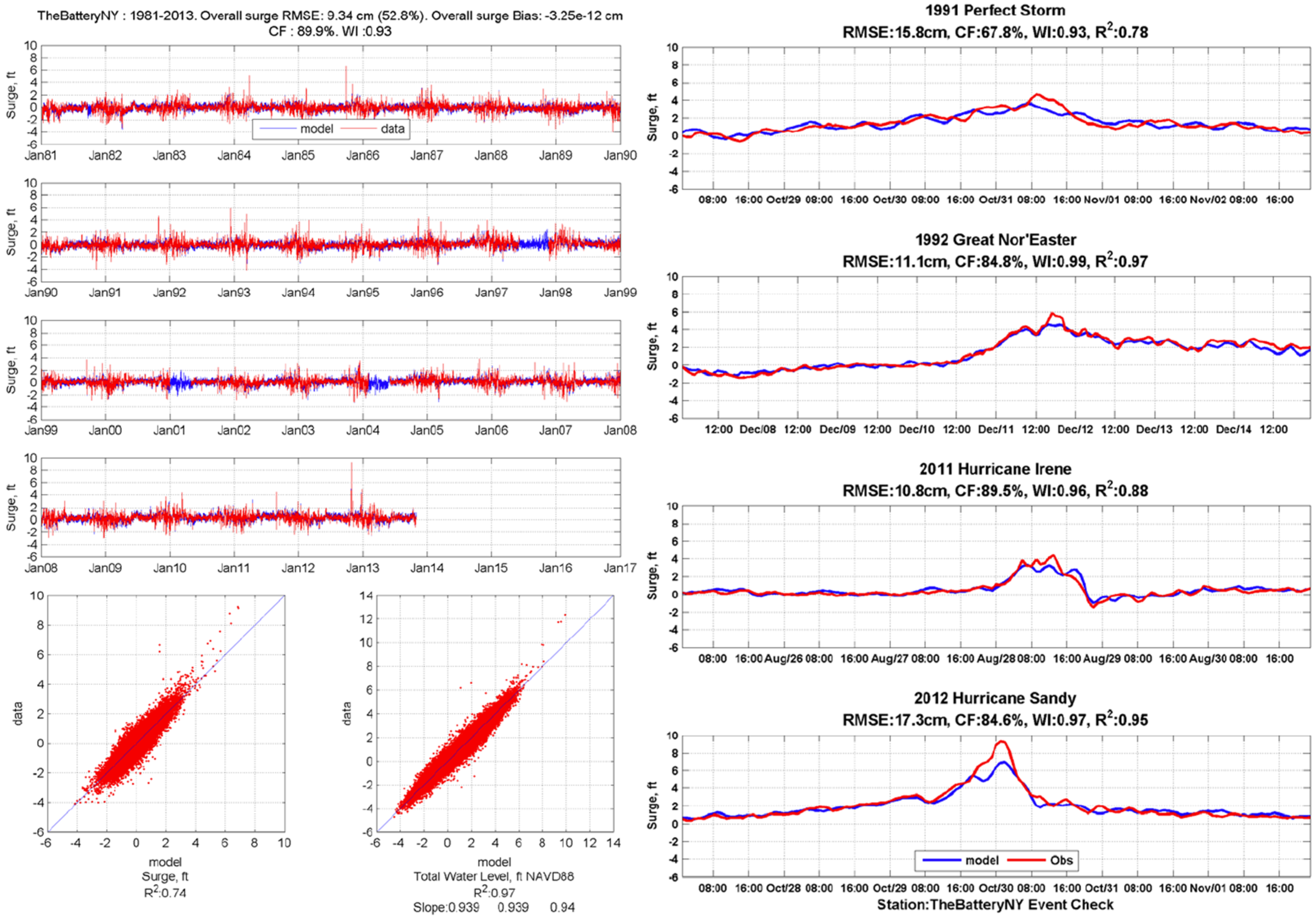
The skill of the comprehensively-forced multi-decadal NYHOPS Hindcast presented in the previous paragraph was overall excellent: across all stations considered, the average Willmott Index of Agreement for storm surge (tidal departure) alone against NOS hourly observations was 0.93, (9 cm Root-Mean-Square-Error, RMSE, 90% of errors less than 15 cm). For water temperature against available NYC DEP and CTDEEP observations, W.I. was 0.99 (1.1 °C RMSE, 99% of errors less than 3 °C). For salinity against NYC DEP and CTDEEP observations, W.I. was 0.86 (1.8 psu RMSE, 96% of all errors less than 3.5 psu).

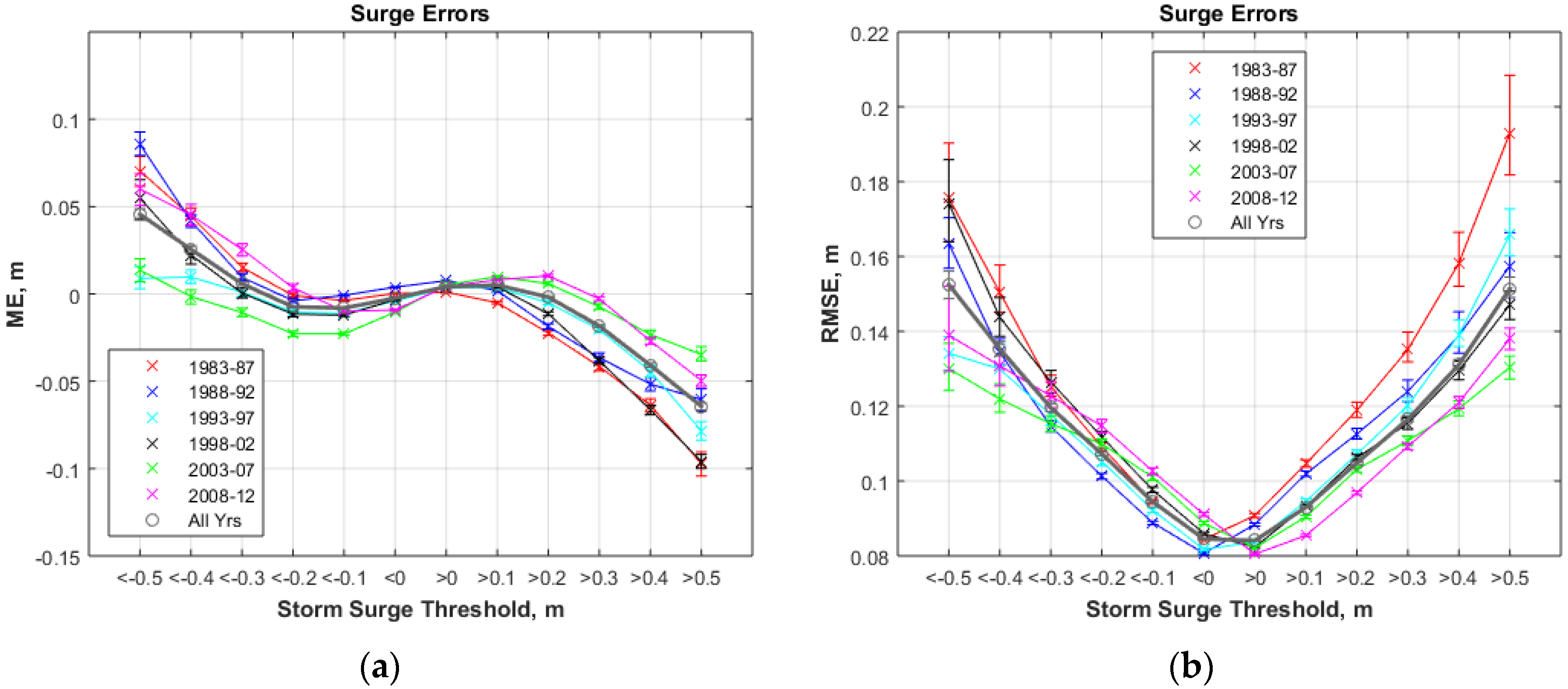
For water levels, model results were reasonable overall, though model errors against hourly observations increased as expected during major storm surge events and Atlantic hurricanes (Figure 9); Figure 9 can also be compared to [16] (Figure 7) and [11] (Figure 5). This error increase with surge magnitude is in part due to the resolution in time (3-hourly) and space (36 km) of the NARR dataset used to provide winds and barometric pressure to the NYHOPS model. Mesinger et al. in 2006 [21] stated expectations for relatively poorer NARR skill during Atlantic Hurricanes. This may in part be due to a presumed increase of the number of observations fed into NARR during the reanalysis process in later years compared to the beginning of the NARR record in 1979. Storm surges during some early events, the Nor’Easter of March 1984 and Hurricane Gloria in 1985 being examples, were under-predicted. The storm surge from the quick transit of Hurricane Bob that devastated New England in 1991 was also not captured. For example, the surge built from 0 to over 5 feet in 4 h at Newport, RI, but the 3-hourly, 36 km NARR record was not able to capture that hurricane well.

The residual water level errors during significant storm surge events appeared to decrease toward the second half of the simulation (Figure 9), even though these later years included some of the highest storm surge peaks in the region’s history during Hurricanes Irene and Sandy. It is also important to note however that the NARR-forced NYHOPS still under-predicted Hurricane Sandy’s peak surge at The Battery by ~2 feet, or ~20% of the observed ~10 feet surge (Figure 4). During the actual event in October 2012 the NYHOPS OFS forecast forced by the deterministic North American Mesoscale (NAM) model at 12 km resolution under-predicted Sandy’s surge at The Battery by approximately 3 feet, while it was within 1 foot when, after the fact, the same model was forced with a more accurate forecast [9] or a high-fidelity reanalysis [10].

Another contributing reason to the apparent increase in the model’s storm surge simulation skill over time may be due to changes in bathymetry and coastline over time, or other morphodynamic or anthropogenic (targeted channel dredging) changes not accounted for in the NYHOPS historic hindcast: the model’s bathymetry is held fixed, and is based on a variety of datasets described in Georgas [14], meant to represent the configuration of the MAB estuaries in the beginning decade of the 21st century. Blumberg and Georgas [13] showed that water levels are quite sensitive to bathymetric uncertainties in the region. Further research is needed in creating a quantitative timeline for such changes, so that future model run versions can account for them.

Table 2. NYHOPS Hindcast Performance metrics summary for water temperature (T) and salinity (S) at regions within LIS and NYNJH.

Water Temperature	Region	Bias, °C	RMSE, °C	W.I.T	CF ≤ 3 °C, %
Long Island Sound CT DEEP LISS Survey	Western Basin	−0.2	1.0	0.99	99
	Central Basin	+0.3	1.0	0.99	99
	Eastern Basin	+0.0	0.9	1.00	100
New York Harbor NYC DEP Surface/Bottom data	Western LIS	−0.4	1.1	0.99	98
	Upper East River	−0.3	1.1	0.99	99
	Inner Harbor	+0.0	1.3	0.99	98
	Lower NY Bay	+0.1	1.3	0.99	98
	Jamaica Bay	−0.2	1.2	0.99	98
NYHOPS OFS 1	NYHOPS 2	+0.0	1.4	0.98	95
Salinity	Region	Bias, psu	RMSE, psu	W.I.S	CF ≤ 3.5 psu, %
Long Island Sound CT DEEP LISS Survey	Western Basin	+0.1	0.5	0.91	100
	Central Basin	+0.0	0.5	0.90	100
	Eastern Basin	−0.6	1.0	0.77	100
New York Harbor NYC DEP Surface/Bottom data	Western LIS	+0.5	1.3	0.77	99
	Upper East River	+0.8	2.2	0.94	93
	Inner Harbor	−0.1	2.8	0.93	89
	Lower NY Bay	−0.9	2.2	0.91	91
	Jamaica Bay	+0.0	1.8	0.71	96
NYHOPS OFS 1	NYHOPS 2	+0.0	2.8	0.77	87

¹ Georgas and Blumberg [15]; ² All stations considered within the NYHOPS model domain, 2007–2009.

summarizes some skill metrics of the NYHOPS historic hindcast against water temperature and salinity datasets at different estuarine regions, and compares that skill to the overall skill of the NYHOPS OFS forecasts from Georgas [14] and Georgas and Blumberg [15]. The multi-decadal NYHOPS hindcast appears to have comparable or better skill than the validated NYHOPS OFS. Note however that the periods compared and the stations used to aggregate errors are not the same, nor is the forcing methodology: the NYHOPS Hindcast used estimates of daily river flows based on observed hydrographs by USGS and three-hourly heat fluxes based on the 36 km NARR, while the NYHOPS deterministic OFS used six-hourly NOAA AHPS river discharge forecasts and three-hourly heat fluxes based on the NAM 12 km forecasts.

Overall hindcast results are well within NOAA standards and skill metrics for T and S (CF > 90%; Table 2). Both water temperatures and salinities were very well predicted. 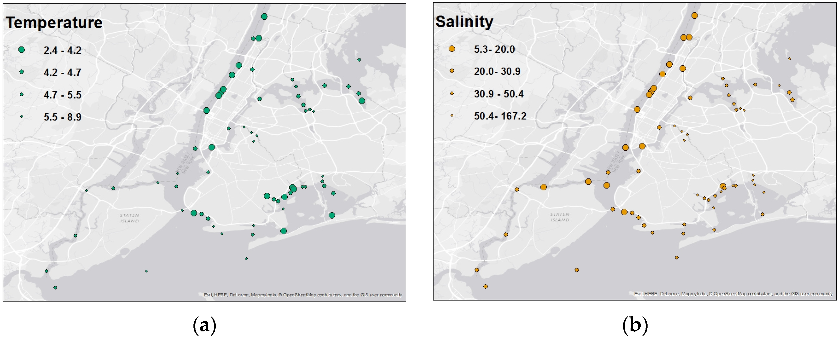Given the greater seasonality in estuarine temperature compared to that of salinity, and the three-hourly meteorological forcing compared to the daily hydrological forcing, the relative RMSE (RMSE divided by the expected range as in Georgas [14]), was higher for salinity than temperature, at an across-station median of 30.9% versus 4.7%, respectively (Figure 10). Figure 10 highlights spatial differences in model skill (as described by the relative RMSE) within NYNJH, by comparing the quartiles of relative RMSE between the hindcast time series and observed time series at NYC DEP Harbor Survey stations. Even though the Hudson River is one of the most dynamic regions in the estuary, it is also one of the best predicted: larger circles in Figure 10 show that the relative RMSE is at its lowest quantile for both T and S there. On the other hand, the model had less skill simulating T and S within some small tributaries such as Newtown Creek and Flushing Creek in the lower and upper East River, respectively, and several tributaries in Jamaica Bay (Figure 10), especially for salinity. These tributaries receive Storm Water flows and occasional Combined Sewer Overflows from the NYC drainage system, non-point sources that are presently not directly simulated by the NYHOPS model but rather estimated as ungagged watersheds. The model’s skill there would potentially benefit greatly through coupling to hydraulic forecast models developed for NYC DEP, although, for a multi-decadal hindcast, changes in the City’s drainage system over time may also need to be accounted for: upgrades to two-times dry-weather-flow by the City’s treatment plants, sewer separation in some areas, and increase in retention storage in others, for example, affect the spatial and temporal distribution of storm water and combined sewage discharged from the hundreds of the City’s interconnected pipes and outfalls.

The model’s dynamics were able to capture more variability than the observation-based MOCHA v2 climatology as evident in relative Brier Skill Scores (BSS) that were positive: 0.48 for temperature and 0.8 for salinity sound-wide. The only exception was for salinity in the Sound’s eastern basin, where the period-average relative BSS was −0.29, indicating that the MOCHA v2 climatology had higher skill than the debiased NYHOPS model there (not shown). Even for that region’s salinity, however, the model’s total RMSE was only 1 psu, of which the remaining bias was 0.6 psu, the average index of agreement 0.77, and the model’s results were less than 3.5 psu away from observed more than 99% of the time. As a comparison, the NOS C.F. standard for simulated salinity is so that errors should be within 3.5 psu for at least 90% of the time [31]. It is important to note here that results in the Eastern LIS basin as well as the Lower NY Bay appear to have been degraded after debiasing (Table 2). The salinity bias correction in the NYHOPS model is consistent with, though slightly smaller than, earlier models in the region: Both the LISS 2.0 and SWEM models used climatological boundary conditions but subtracted 2.0 psu. It is possible that the SODA climatology is biased high for salinity, but the results from the two regions closest to the open boundary in Table 2 may indicate otherwise. Also, like earlier models, the NYHOPS Hindcast does not include the precipitation-evaporation imbalance over the Sound’s waters, submarine groundwater discharge, or other aquifer-related freshwater sources. Although these diffuse sources have been estimated to contribute a total freshwater flow over the Sound that is an order of magnitude smaller than the Connecticut River [35,36], they may in any case contribute somewhat to the high-salinity bias in the models. Further research is needed to quantify these contributions, and explore the reason for that consistent bias in models of the region.

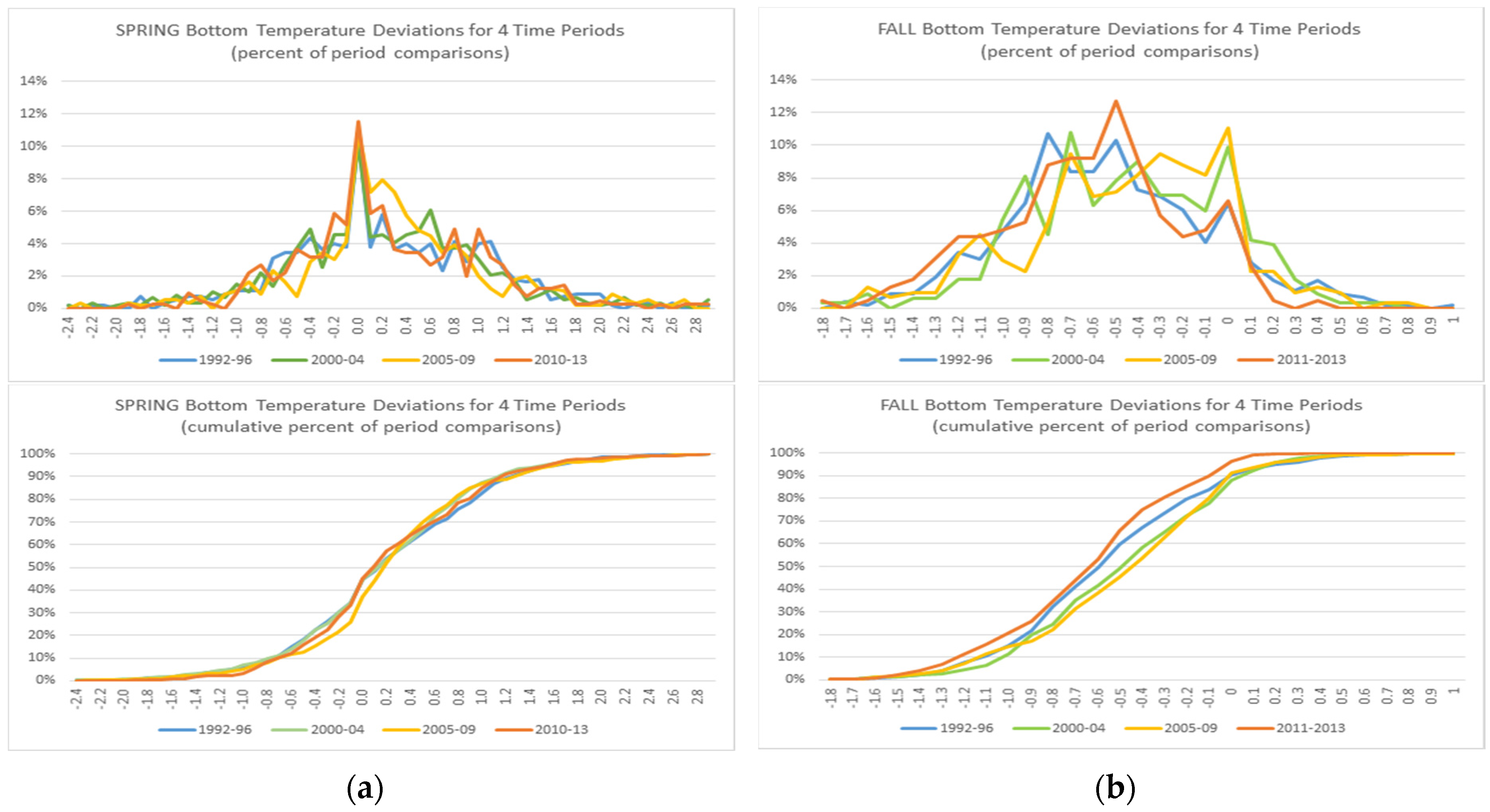
A very important finding of the research is that the NYHOPS model’s skill in simulating water temperature, validated against historic data from the LIS bottom trawl survey, did not drift over the years. The error histograms and PDFs included in Figure 11 for four consecutive periods during both the (a) spring and (b) fall survey periods, show that there was no clear indication of an earlier period having greater error than a later one, or vice versa, unlike what was shown earlier for storm surge. A similar analysis against NYC DEP Harbor Survey data in NYNJH for subsequent five-year periods from 1983 to 2012 also did not indicate drift in skill for surface or bottom T nor S (Supplementary Material, Pages 10–18). This is a significant and encouraging finding for multi-decadal model applications used to identify and research climatic trends and causalities. Figure 11 also shows that the median error in simulated bottom temperature in LIS was low for both the spring (+0.1 °C) and the fall (−0.5 °C) surveys, with only few predictions being further than ±1.5 °C from observed samples.

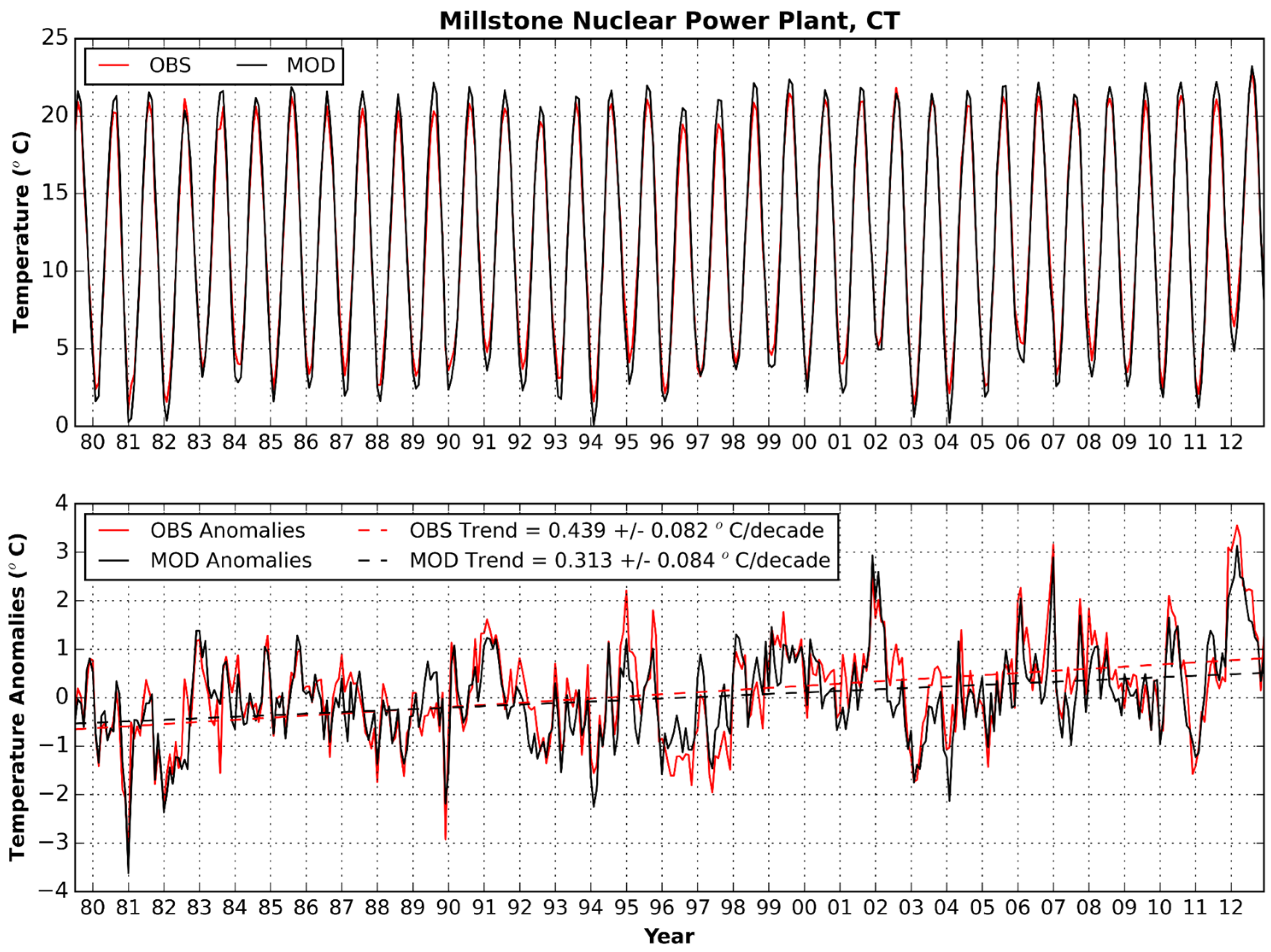
The lack of model drift was further supported through comparison of the simulated water temperature time series to the one and only long-term water temperature record for Long Island Sound taken at a near-surface location just outside the Millstone Power Plant at Millstone, CT (Figure 12). The central estimate for the linear trend of the observations at Millstone (0.439 °C/decade) was somewhat higher than the linear trend of the NYHOPS hindcast there (0.313 °C/decade), and the simulated annual range was somewhat higher than observed (Figure 12), however the two trends were not different at the 95% confidence level. Figure 12 shows that water temperature was simulated very well throughout the hindcast period. It also shows clearly that temperatures have been increasing at the site and that 2012 was the warmest year in both the simulated and observed record.

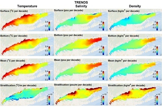
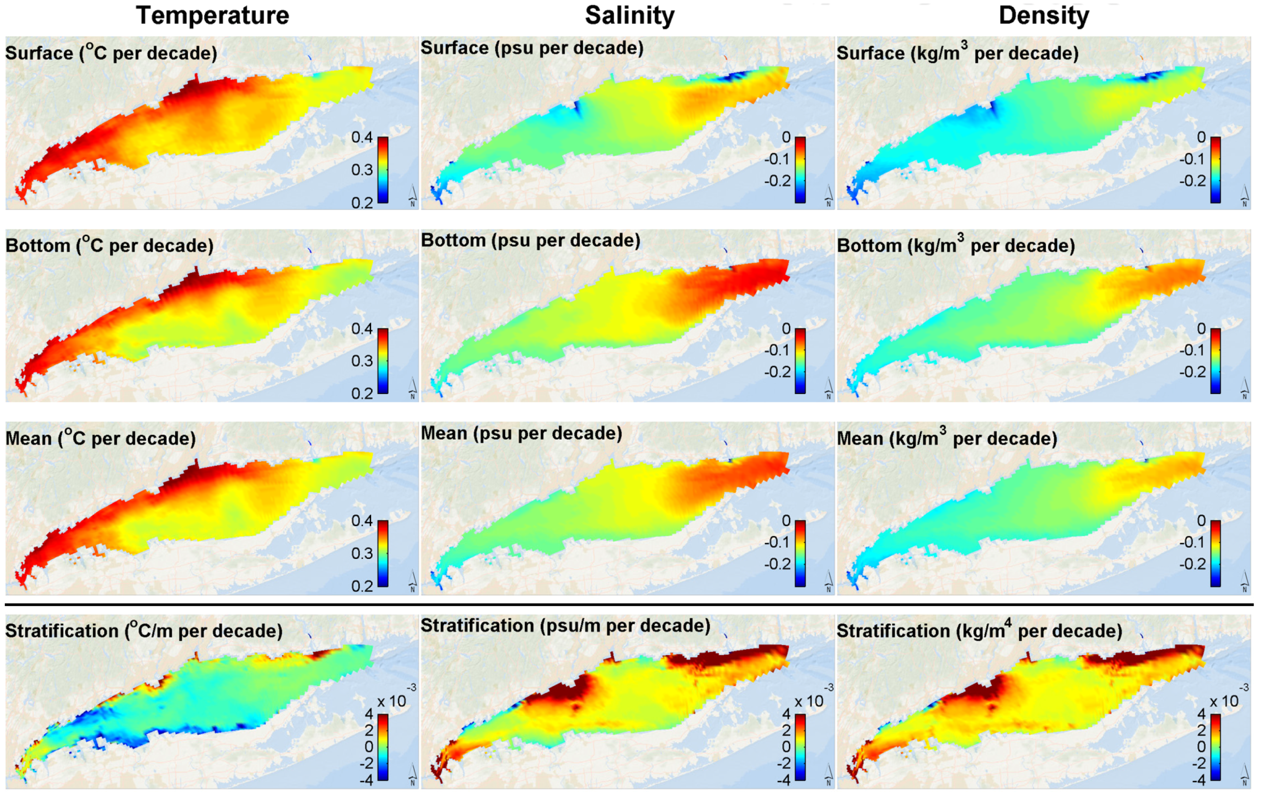
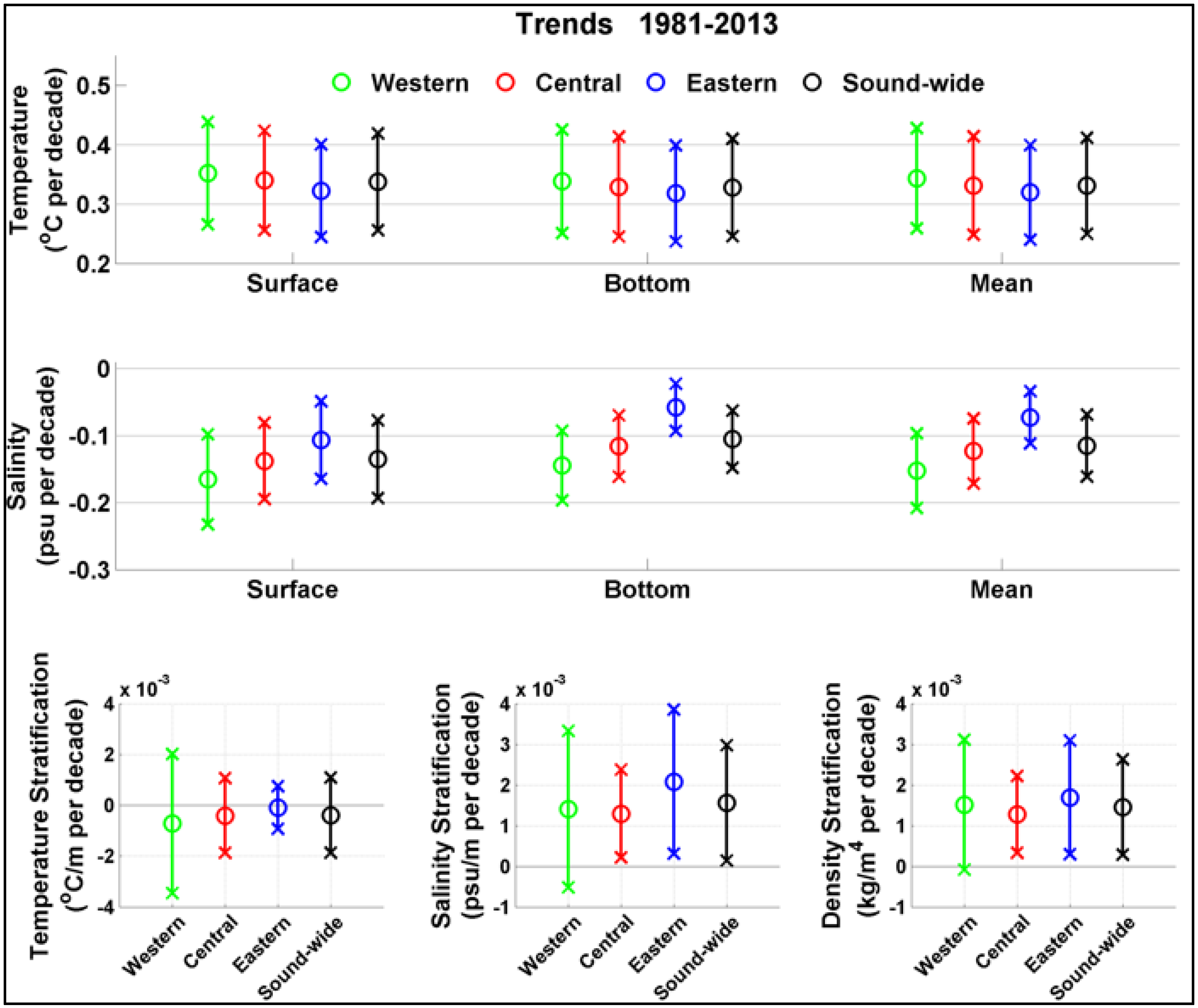
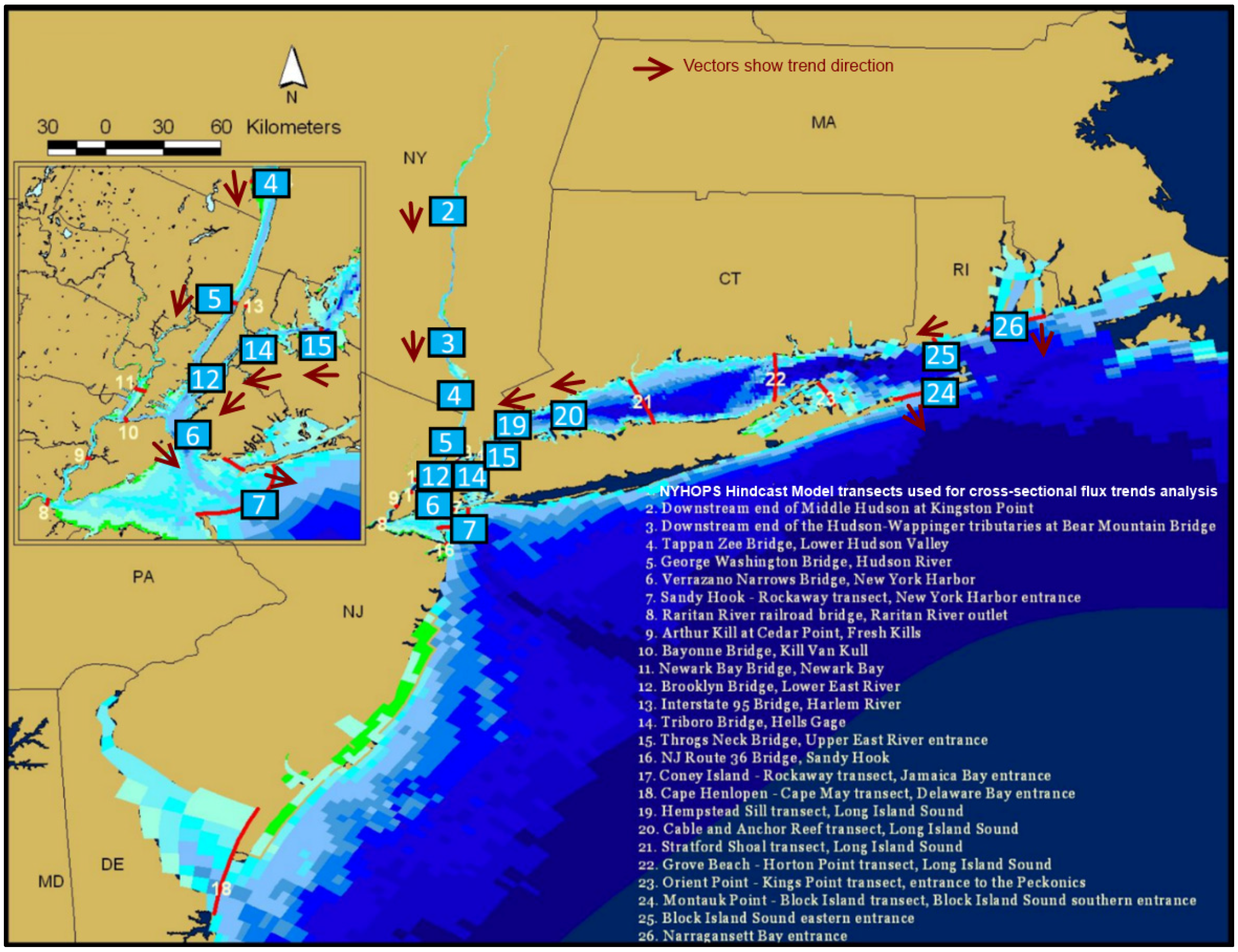
NYHOPS model results were then used to quantify linear, water temperature, salinity, and stratification trends for LIS in the hindcast period between 1981 and 2013. Spatially averaged trends over the three Long Island Sound management basins (east, central, west), and the Sound as a whole are shown in Figure 13, with confidence intervals, while the spatial variation on the NYHOPS grid cell level is seen in Figure 14. Statistically significant warming and freshening trends (Figure 13), non-stationary trends in volumetric fluxes across the western and eastern basins of the Sound (Figure 15), and an associated statistically significant increase in stratification (Figure 13 and Figure 14) have all occurred within the hindcast period. Based on the NYHOPS hindcast, in the Long Island Sound basin, surface air temperatures, contributing river temperatures, and receiving LIS-basin-wide water temperatures (0.34 ± 0.08 °C per decade) have all seen significant increases between 1981 and 2013, more so on the shallower north shore and western Sound than the south shore similar to [37]. The basin wide average is comparable to the 0.30 °C per decade rate reported for SST at the Gulf of Maine [3]. The increase in major freshwater rivers mentioned in Section 2 may have led to the Sound overall becoming somewhat fresher (a statistically significant trend of 0.12 ± 0.05 psu/decade), especially near river mouths at the surface (Figure 14), increasing stratification and changing long-term volumetric transport fluxes in the basin in a statistically significant, nonstationary way (Figure 15). Further research is needed to deduce whether these trends are expected to continue into the future.

5. Conclusions

The NYHOPS model’s application to hindcast storm surge and 3D water temperature and salinity conditions in its region over three-and-a-half decades was validated against observations from multiple agencies, as well as climatology: the average index of agreement for storm surge alone was 0.93 (9 cm RMSE, 90% of errors less than 15 cm); for water temperature, it was 0.99 (1.1 °C RMSE, 99% of errors less than 3 °C); and for salinity, it was 0.86 (1.8 psu RMSE, 96% of errors less than 3.5 psu). The model’s skill in simulating bottom water temperature, validated against historic data from the Long Island Sound bottom trawl survey, did not drift over the years, a significant and encouraging finding for multi-decadal model applications used to identify climatic trends. However, the validation revealed residual biases in some areas, including small tributaries that receive urban discharges from the NYC drainage network. With regard to the validation of storm surge at coastal stations, both the considerable strengths and remaining limitations of the use of NARR to force such a model application were discussed.

Through the comprehensively forced, and herein extensively validated, multi-decadal simulation for Long Island Sound’s physical environment performed using Stevens Institute of Technology’s NYHOPS hindcast model, temperature increases in Long Island Sound over the past three-and-a-half decades have been confirmed and have been found to be statistically significant. The linear trends have also been found to be quite high (0.34 ± 0.08 °C per decade) and comparable to ones in the Gulf of Maine [3]. Further research is needed in identifying the cause for this increase in temperatures. Source allocation and further sensitivity runs using the NYHOPS model may aid in testing hypotheses in the future.

After extensive model validation and debiasing, an online THREDDS Data Server (http://colossus.dl.stevens-tech.edu/thredds/catalog.html) was set up to serve the NYHOPS model’s results in NetCDF format over the web using the OPENDAP protocol, enabling similar analyses through open access to daily averaged or monthly averaged time series for all the gridded hindcast physical variables in or over the NYHOPS region that includes NYNJH and LIS.

Fisheries management has traditionally sought to reduce harvesting levels in response to low stock biomass, in its goal to maintain long-term fishery productivity [38]. More recently, accounting for non-stationary environmental forcing has started being considered in stock assessment and management ([39], pp. 131–147) with the realization that a failure to account for shifts in climate that can alter population dynamics can lead to stock collapse as with the Gulf of Maine cod fishery [3]. This progress has been facilitated by new population dynamics models that consider temperature-dependencies and an improved understanding in climate-fisheries teleconnections brought about through advances in environmental modeling.

NYHOPS Hindcast results are in demand to support this kind of fisheries research through coupling to habitat suitability indices, population models, water quality models, or to provide boundary conditions to higher resolution embayment or tributary circulation models. The datasets are also presently used to inform ongoing research in climate teleconnections and ecosystem change through exploratory statistical analyses linking regional fisheries abundance to global climate indices. The authors are encouraged by the early interest in these datasets.

Simulated climatologies (mean simulated climate conditions averaged over the three decades of the NYHOPS hindcast period) for two- and three-dimensional fields such as water temperatures and salinities, were also generated, and included in THREDDS. Included on the same THREDDS server is a “daily anomaly” dataset, comparing the latest operational forecast of the NYHOPS OFS model to the 1981–2013 debiased daily climatology, so that interested parties can see how different yesterday and the next three days are predicted to be from the climatological average, enabling near-term tracking of anomalous patterns in Long Island Sound. Fish-surveying strategies may also be improved through the use of the NYHOPS model forecasts: NYSDEC and NMFS routinely already use the model’s predictions for adaptive sampling in the Hudson River estuary and the Mid-Atlantic Bight Apex. Visualization is easy with off-the-shelf free software, such as NASA’s Panoply, accessing the datasets over the web.