Application of a Spectral Wave Model to Assess Breakwater Configurations at a Small Craft Harbour on Lake Ontario

Abstract

A surface wave model using three nested grids is applied to the eastern end of Lake Ontario to investigate wave propagation from an open lake environment to a small craft harbour protected by a breakwater. The Simulating WAves Nearshore (SWAN) spectral wave model, coupled with the Delft3D hydrodynamic model, is applied to simulate a series of storms in November, 2013. The model results are compared to observations from two pressure sensors, and used to quantify wave properties around existing and future breakwaters to evaluate the bulk changes to the harbour configuration. Overall, the results indicate that the rubblemound breakwater reduces wave heights in the existing harbour by 63% compared to no breakwater, and that the addition of a surface breakwater extension could reduce wave heights by an additional 54%. Wave height attenuation was found to be highly dependent on the incident wave direction relative to breakwater orientation. The spectral wave model is useful for simulating wave transformation for broad directional spectra in wind-sea conditions over large scales to semi-protected areas such as small craft harbours.

1. Introduction

Breakwaters are marine structures built to attenuate the height and reduce the energy of incoming waves, protecting important areas along a coast such as marinas or harbours. Recent work [1] describes how breakwaters can significantly reduce wave loading on structures, by using a Smoothed Particle Hydrodynamics (SPH) model to calculate hydrodynamic forces. However there are a number of physical processes that occur due to wave transformation around these structures that make predicting wave height and energy behind them complex, and difficult to predict without detailed information regarding the bathymetry and incident wave conditions. Several numerical models have been developed to compute wave transformation over changes in bathymetry and into semi-protected areas, such as REFDIF [2], and the Simulating WAves Nearshore (SWAN) model [3]. For this study SWAN is used to perform wave predictions over a large scale, from an open lake environment to a small craft harbour (SCH) protected by a breakwater, and includes wave-driven circulation and storm surge by coupling with Delft3D [4]. This model has been used to successfully model wave behaviour around breakwaters in previous studies, e.g., [5]. SWAN has been shown to model the wave and current behaviour in Lake Ontario effectively [6], as well as other areas with complex bathymetry [7]. SWAN has also been applied to effectively model wave behaviour around a detached breakwater in comparison with laboratory and field data [8].

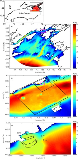
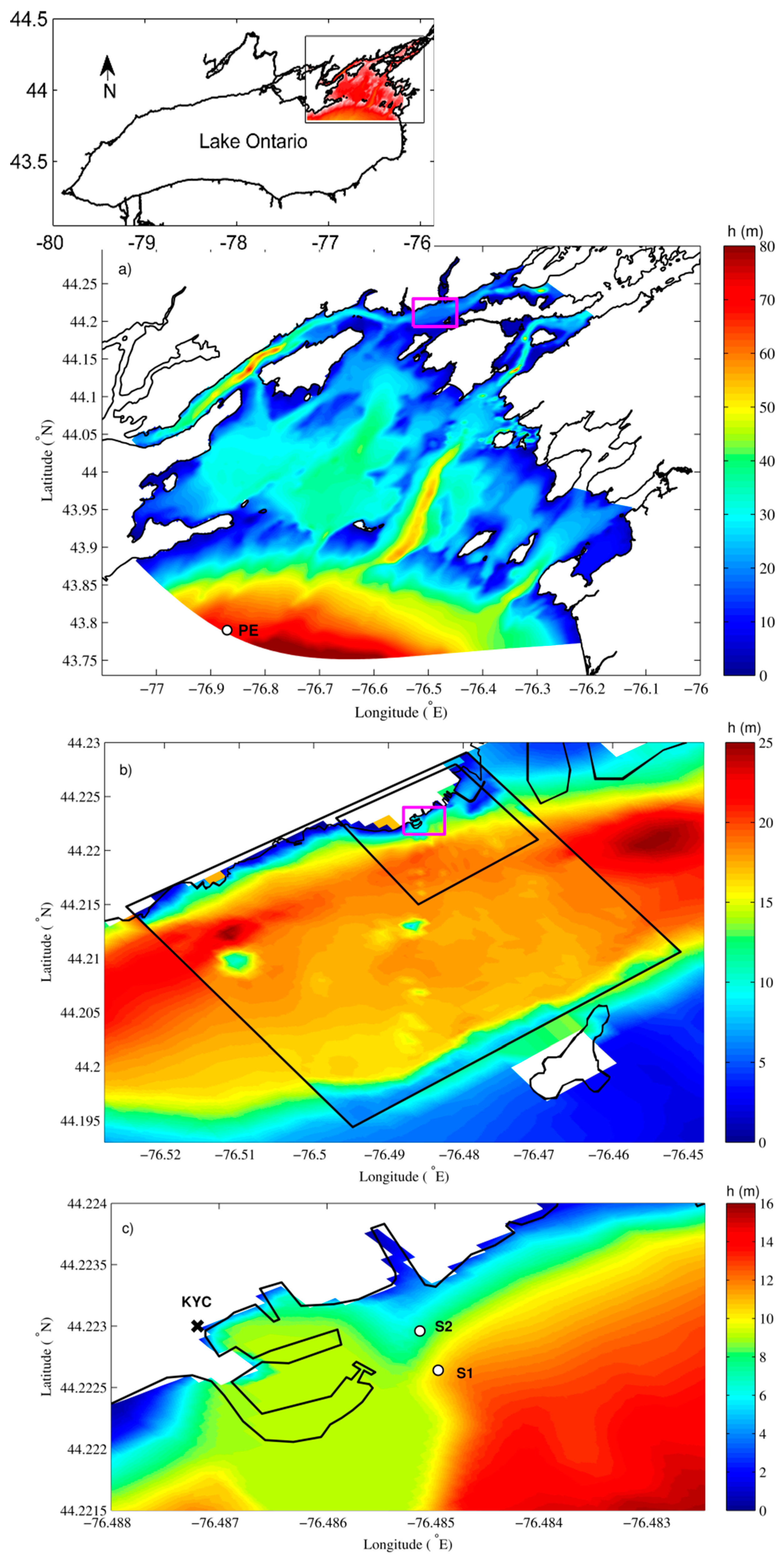
The wave climate in eastern Lake Ontario is dominated by storms with wind-generated waves with significant wave heights up to 5 m [6], and lake-scale wind-forced storm surge and circulation [9]. The region of the present study is the northeast end of Lake Ontario (Figure 1a), Kingston Harbour (Figure 1b) and the area surrounding the Kingston Yacht Club (KYC) (Figure 1c). This is a region in which there have been recent investigations using numerical models such as Delft3D [6,9], ELCOM [10] and FVCOM [11]. The purpose of this study is to investigate how effectively SWAN can simulate surface waves over a large scale from an open lake, around islands and over channels and shoals, to a SCH protected by a breakwater. A second objective is to examine how wave characteristics change in the absence or presence of different breakwater configurations, and to investigate whether or not a pile-supported surface breakwater extension that allows some wave transmission is beneficial for a possible future expansion of the SCH in Kingston Harbour. This paper is organized as follows: the wave observations and the numerical models are described in the Methods section. The Results section outlines the model predictions compared to wave observations, and wave propagation around different breakwater configurations. A discussion of these results is covered in the Discussion section, and conclusions are provided in the Conclusions section.

2. Methods

In this study the approach includes wave measurements at two sites near the existing rubblemound breakwater, and the application of numerical models to simulate waves in eastern Lake Ontario with higher resolution in Kingston Harbour and around the Kingston Yacht Club.

2.1. Wave Observations

Wave data were recorded by two 2 Hz RBR TWR-2050 pressure-temperature sensors in two locations east of the KYC breakwater (Figure 1c). S1 was located just outside of the existing rubblemound breakwater’s protected area in a mean water depth of 10 m, and S2 was situated in the protective lee (for waves from the SW or W directions) of the existing breakwater at a mean depth of 9 m. The pressure sensors sampled at 2 Hz, and were configured to do wave bursts for 20 min per hour. The sensors were deployed for four months (1 August to 30 November, 2013) in two deployments of two months. 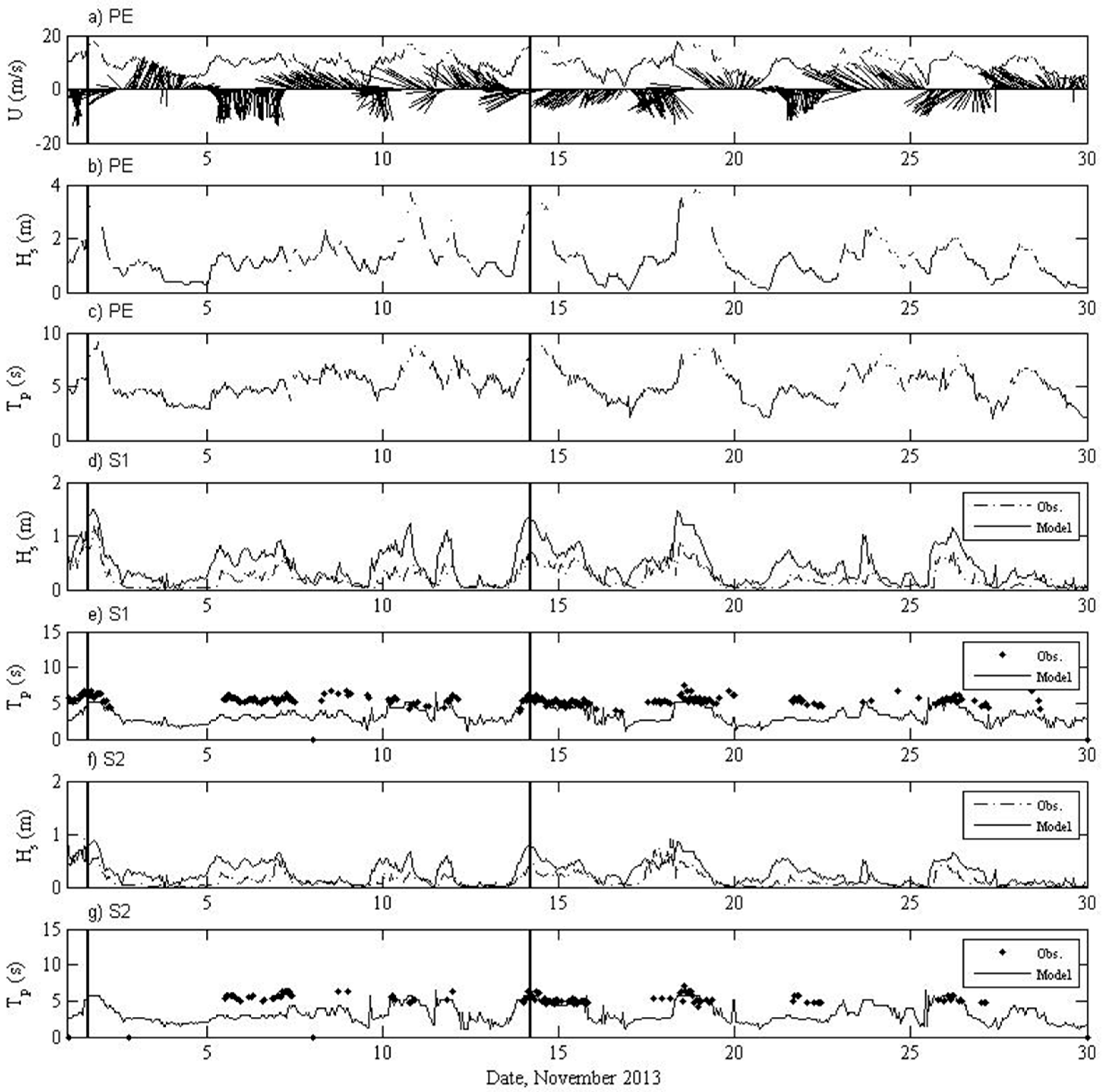Pressure spectral distributions were observed at each site, from which sea-surface statistics including significant wave height (H_s) and period (T_p) were calculated. Due to attenuation of wave energy with depth, pressure spectra observed near the bottom were valid up to a frequency cut-off of 0.38 Hz, resulting in observations of only the longer period waves (T >2.6 s) that typically have peak periods of greater than 4 s. Wind and wave conditions are shown in Figure 2 for the month of November, which had the largest storm events in the observation period. During storm events, waves reached significant wave heights of 1.6 m at S1, and 0.9 m at S2, and peak periods were 5–7 s at both sites.

Data from the Prince Edward Pt. Buoy (buoy C45135) at PE (Figure 1a) [12], was used to determine wind conditions and offshore wave conditions. The observed wind speed and direction, significant wave heights, and peak wave periods are shown in Figure 2. Wind speeds reached almost 20 m/s during several storm events, the largest waves in the lake reached significant wave heights of approximately 4 m, and the peak wave periods for large events ranged from 7–9 s at PE. Observations at sites S1 and S2 indicate that there is no change in wave height between the sites for waves from the south, and therefore waves are not affected by the existing rubblemound breakwater, and are only limited by the short fetch across Kingston Harbour. For waves arriving from the west or southwest, the reduction in wave height over a short distance of approximately 20 m from S1 to S2 indicates that the existing breakwater is currently providing protection for the SCH from a significant amount of incident wave energy.

2.2. Numerical Models

SWAN is a third-generation spectral wave model that predicts wave conditions in shallow regions, accounting for all relevant generation and dissipation processes, as well as wave-wave interactions. The wave field evolution is described by the action balance equation [3] where wave action density is transported as a function of time, horizontal space, wave frequency, and wave direction, and sources (wind) and sinks (dissipation) induce local changes to the wave spectrum. To estimate wave behaviour around and through structures such as breakwaters using SWAN, obstacles can be defined [13] with specified transmission (K_t) and reflection (K_r) coefficients. These obstacles are modelled as linear elements in the computational area, and affect the wave field by reducing wave heights, causing wave reflection and causing diffraction around their ends. Transmission is calculated for waves over submerged structures or by using a constant transmission coefficient for permeable structures. Diffraction is accounted for using a phase-coupled refraction-diffraction approximation [13], although the effects have been shown to be less pronounced for broad directional spectra in wind-sea conditions [8]. Delft3D is a 3-dimensional modelling system that simulates the water levels and currents, and can also be applied to simulate sediment transport, morphological change, and water quality [4]. SWAN can be coupled with Delft3D at a specified time interval, and perform wave computations that include wave-current interactions and the effects of changing water depths on wave refraction and breaking.

For this study, SWAN is used to predict wave behaviour in the eastern end of Lake Ontario using a system of three curvilinear nested grids in spherical coordinates and forcing by both winds over the domain and waves at the open boundary. A coarse grid with a resolution of approximately 270 m was developed for the eastern region of Lake Ontario, covering the area in Figure 1a. Time-varying wave forcing conditions obtained from the buoy at PE were applied to the curvilinear southern boundary (Figure 1a). The wave boundary conditions are described using the time-varying bulk wave parameters observed at PE to construct a JONSWAP wave spectrum with a peak enhancement factor of 3.3 and directional spreading using a cos-squared function. A medium grid with a resolution of approximately 90 m was nested in the coarse grid and covered Kingston Harbour (Figure 1b). A fine grid with resolution of 30 m was nested in the medium grid to provide the highest resolution around KYC (Figure 1c), with further local refinement around the breakwater to a resolution of 10 m and several model grid points between S1 and S2 to account for differences between these closely spaced sites. This finest numerical can resolve the essential features of the harbour structures and changes in wave properties within the harbour.

Wind conditions were obtained from the PE buoy. To ensure spatial uniformity of the wind field, the wind observations at PE were compared with data collected at the Kingston Airport [14] and with wind observations at KYC. The average difference in wind speed between the three sources was less than 4 m/s suggesting that the wind field is near-uniform in space over the area, and the buoy observations were selected for model input due to the completeness of the dataset over the study period. The model spectrum was discretized using 24 logarithmically-spaced frequency bins from 0.05 to 1.00 Hz and 36 directional bins with 10° spacing. Bottom friction was parameterized using the JONSWAP formulation with a coefficient of 0.067 m²·s⁻², the default value in SWAN. Whitecapping is formulated according to a saturation-based dissipation that is dependent on the local wave number [15]. SWAN was run in stationary mode, and was coupled to Delft3D by communicating every 60 min of simulation time. Delft3D operated using a time step of 6 s to ensure stable computations according to the Courant condition. Other model parameters in SWAN and Delft3D were defined following previous results on detailed validation of the coupled model with wave and current observations in the Kingston Basin of Lake Ontario [6,9]. The models are both forced by the time-varying winds, which generate waves and in SWAN and wind-driven circulation and storm surge in Delft3D.

3. Results

The following section outlines the results of this study. First, the model results are compared with observed data from the pressure sensors to validate the model. Second, the impact of different breakwater configurations on wave conditions in the harbour are investigated.

3.1. Comparison with Observations

The model was run for the months of October and November, with spectral output at the two sensor locations. The significant wave height and peak period at each site are compared with observations in Figure 2 for the month of November, a time period with the largest observed wave heights. Spectral peak wave periods determined from observations that were less than 4.3 s are excluded from analysis due to attenuation of wave energy with depth for short period waves. In general the observed and predicted wave statistics were in good agreement during storm events, particularly when H_s > 0.5 m at S1. 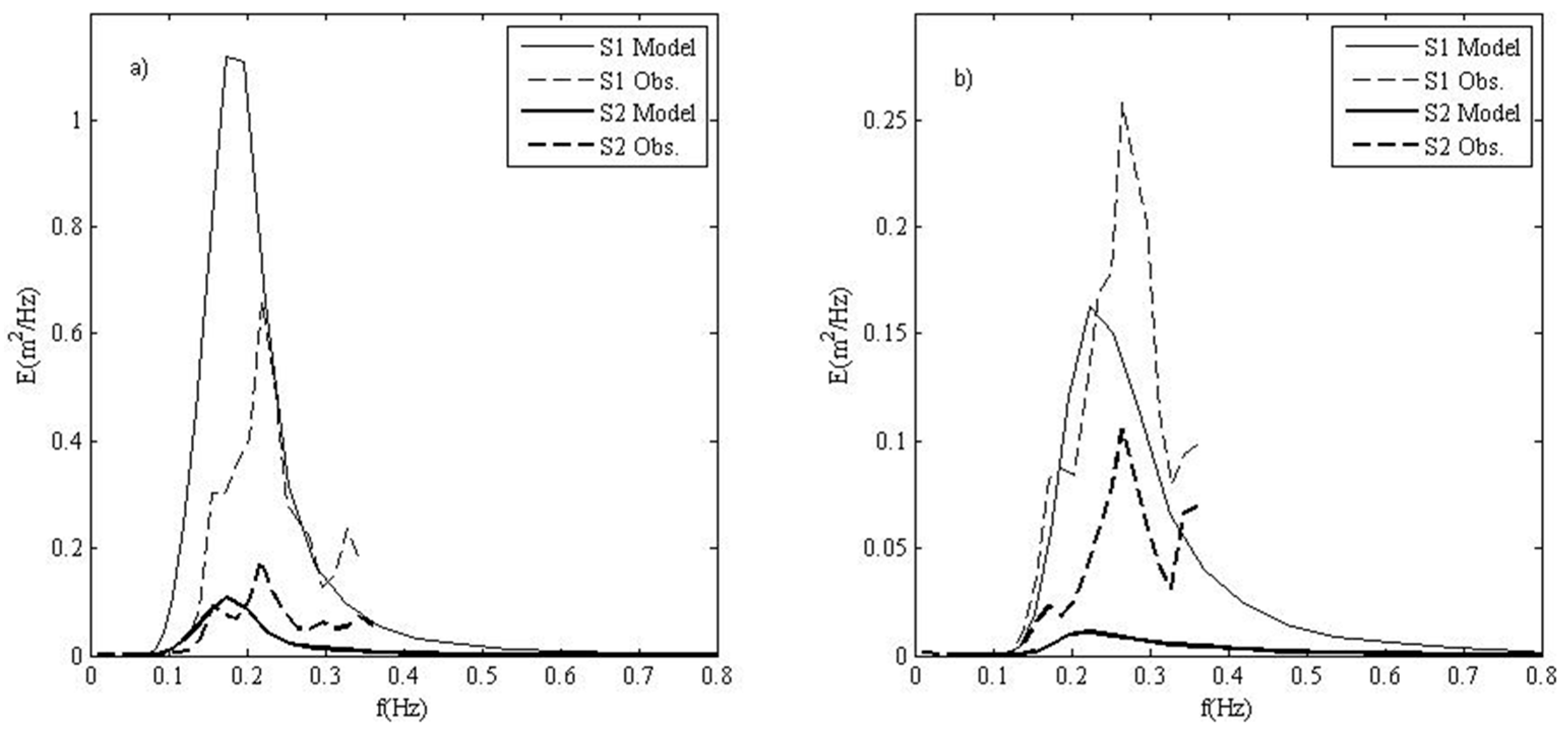The measured significant wave heights are typically smaller than the true H_s and the measured wave periods are generally larger than the true T_p for the smaller wave events with short peak wave periods, since pressure sensors on the lake bottom cannot measure energy in the high frequency part of the wave spectrum [15] due to attenuation with depth that is frequency dependent [16]. For the short wave period conditions, the pressure oscillations at the bed due to the surface waves are very small and therefore all frequencies above 0.38 Hz are excluded from analysis. This is shown in Figure 3, where the model spectra are compared with the observations only at frequencies below the cut-off. Major discrepancies occur between measurements and models as indicated in Figure 2 and Figure 3. The pressure sensors in deep water, for these wave periods, do not fully capture the surface wave signal and are not the most appropriate choice of sensor under these conditions due to the attenuation of the wave-induced pressure signal.

However, the model is a useful tool to simulate the wave conditions over a wider frequency range then observed by the pressure sensors, and additional field measurements using other methods should be collected before detailed design of any coastal structure.

3.2. Breakwater Configurations

Three idealized breakwater configurations were simulated and are shown in Figure 4, including: (1) the past scenario with no structures; (2) the present-day scenario with a rubblemound breakwater; and (3) a possible future scenario with the addition of an idealized 40 m long pile-supported surface breakwater extension with a 10 m “L”-dock, connected to the end of the existing rubblemound breakwater. The breakwaters were modelled as obstacles in SWAN, where sub-grid scale elements are used to define the edges of the structures. The rubblemound breakwater was modelled as a dam with no transmission allowed (valid for this bottom-founded rock structure at KYC), diffuse reflections (a reflection coefficient of 0.5) and a height of 2 m, and a breakwater slope of 1:3/2. The breakwater extension was modelled as a semi-permeable sheet with K_t = 0.7.

The transmission coefficient for the idealized pile-supported structure at the water surface was selected based on a relationship between the wave transmission coefficient and wave steepness (H/L) for breakwaters at the surface [17]. For a single-pontoon rectangular-section breakwater that is moored with chain, physical model experiments indicated that K_t = 0.6–0.8 apply over a range H/L = 0.03–0.10. The present numerical results without the breakwater extension indicate that at S1, located closest to the site of the breakwater extension, the mean value of H/L is 0.05 and therefore an average wave transmission coefficient of 0.7 was selected to simulate the obstacle in SWAN. It is noted that wave transmission past a rigidly-moored surface breakwater is a function of the breakwater geometry (width, draft, cross-sectional shape, mooring design) and the incident wave conditions (wave period, relative wave angle), and that other modelling techniques could be applied to determine breakwater performance over a range of conditions. The single value of 0.7 is selected conservatively for use in SWAN to apply to the worst-case conditions, where the longer period waves arrive from the SW a high angle from normal to the structure. For shorter period (fetch-limited) waves from the S that are normally incident, a lower transmission coefficient of 0.5 would be appropriate.

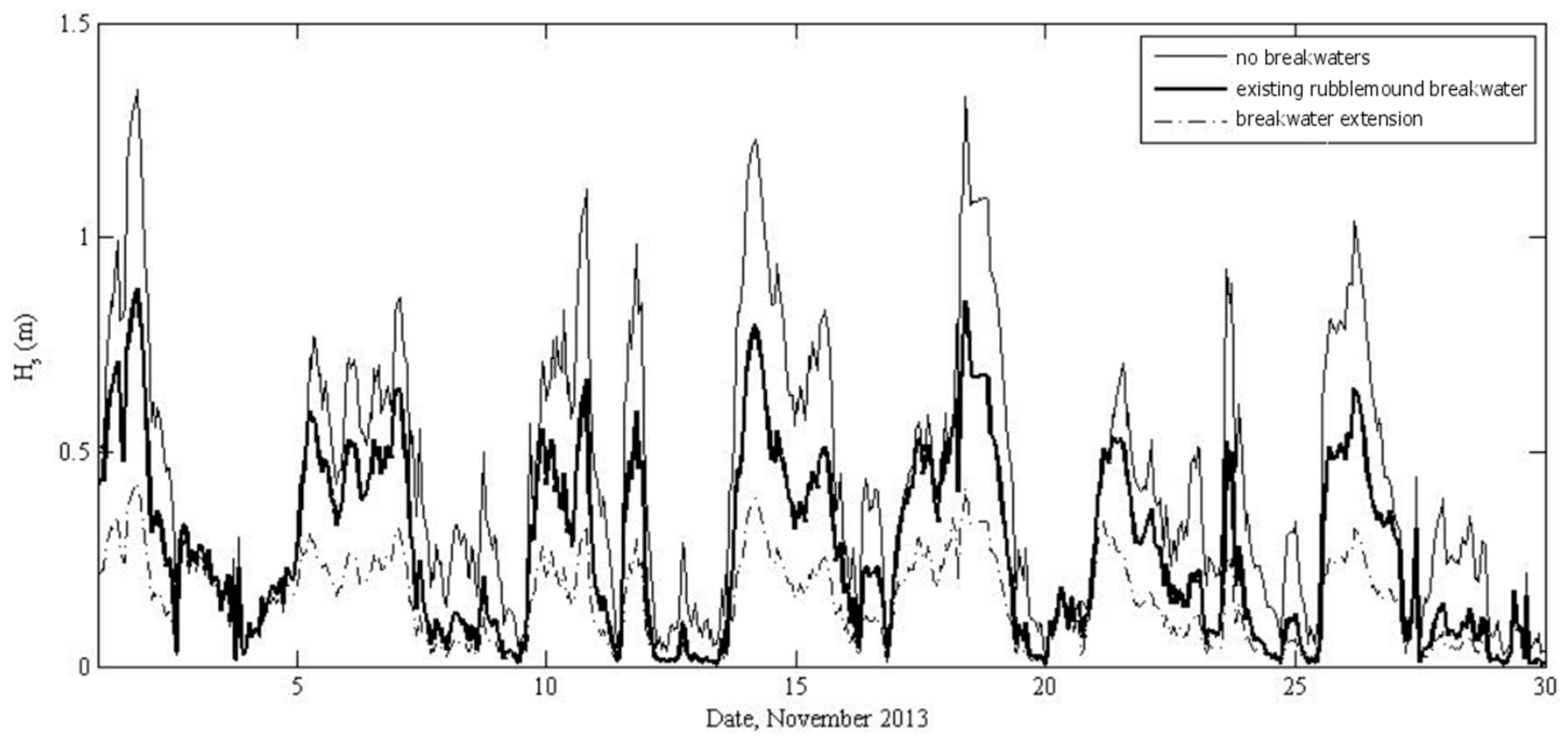
The three different breakwater configurations each dramatically influence the wave height at S2, indicated in Figure 4 for a storm event on 1 November. This is also shown in Figure 5 for the time-series corresponding to the month of November. Averaged over the month, wave heights would be 0.16 m (63%) higher without the rubblemound breakwater and the addition of a breakwater extension would reduce the wave heights by a further 0.12 m (54%) where 100% represents total reduction of H_s to 0 m. There was no difference in the peak wave period between the three breakwater configurations.

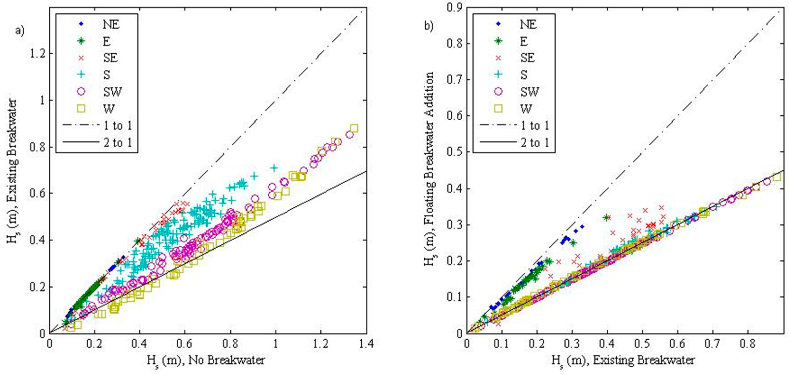
The reduction in wave height in the harbour at S2 is sensitive to the incident wave direction as indicated in Figure 6. Waves coming from NE, E, and SE directions are not affected by the presence of the rubblemound breakwater, while the breakwater causes an increasing amount of wave height attenuation as the wave direction rotates from S to SW to W (Figure 6a) compared to the case of no rubblemound breakwater. For the case when the breakwater extension is connected to the end of the rubblemound breakwater, (Figure 6b), there is no difference from the rubblemound only case for waves from the NE and E directions, but waves from the SE are reduced in height by 20%–40% and waves from S, SW and W directions are reduced by a nearly constant 50%. The significant wave height inside the future harbour that is protected by the breakwater extension do not exceed 0.45 m, suggesting that this type, length and location of structure is effective in wave attenuation in the SCH.

4. Discussion

The application of a spectral wave model like SWAN, coupled to Delft3D, to predict wave transformation in a SCH requires accurate estimation of the transmission coefficient for permeable structures. In this study a representative transmission coefficient is used for the surface breakwater extension, and the bulk results are compared to the case of no structure. Using linear obstacles to simulate breakwaters resulted in useful predictions of wave behaviour in a SCH. However, obstacles are thin relative to the horizontal of individual grid cells in the model, and do not exactly resolve the size and shape of the structures. To more accurately predict wave condition inside a SCH, the structures should be larger than the grid cells and changes in bathymetric features, suggesting very high (and computationally limiting) horizontal resolution. However, creating obstacles as relatively simple, linear elements to define the edges of the structures allows the reflection and transmission to be controlled and the structures to be evaluated over a long time-series of realistically varying wave conditions.

The reduction in significant wave height inside the SCH that occurs with both the existing rubblemound breakwater and future breakwater extension is explained primarily by the shapes and orientations of the two obstacles. The rubblemound breakwater curves and encloses that harbour effectively, protecting the S2 site from waves coming from the W and SW directions. However, wave diffraction occurs around the tip of the breakwater and therefore some wave energy does enter the harbour. The entrance, which faces east, leaves the harbour exposed to waves coming from the E and SE directions. The breakwater extension, which extends eastward along the southern side of the harbour, will provide additional protection for the harbour in the region of site S2. It attenuates the wave height from the SE and S directions far more effectively than the rubblemound breakwater alone, resulting in smaller wave heights in the SCH. Waves from the SW approach at a high angle relative to the breakwater extension and have the longest wave periods of 5–7 s. These waves are likely to transmit the greatest amount of energy past the breakwater extension at the surface, and other modelling techniques could be applied to investigate wave transmission for varying incident wave periods and relative wave directions.

5. Conclusions

This study investigates the SWAN model’s ability to simulate surface waves from an open lake to a small craft harbour (SCH) protected by a breakwater by comparison with pressure sensor observations, and how wave behaviour changes in the SCH for different breakwater configurations. The pressure sensors did not fully capture the surface wave signal in deep water and were not the most appropriate choice of sensors under these conditions due to attenuation of the wave-induced pressure signal with water depth. However the model was a useful tool to simulate the wave conditions over a wider frequency range then observed by the pressure sensors, and additional field measurements using other methods should be collected before detailed design of any coastal structure.

Obstacles were used to model the existing rubblemound breakwater (no transmission and a reflection coefficient of 0.5), and a possible future breakwater extension at the surface (a conservative transmission coefficient of 0.7) to further reduce wave agitation in the harbour. SWAN, coupled with Delft3D to simulate wind- and wave-driven water level changes and circulation, was able to predict wave heights inside the harbour area protected by the existing rubblemound breakwater, but tended to over-predict the significant wave height and under-predict the peak wave period. Numerical tests were conducted with three breakwater configurations (no breakwater, existing rubblemound breakwater, and existing rubblemound breakwater with a 40 m long breakwater extension). The results indicate that the existing rubblemound breakwater reduces wave heights in the SCH by 63% (0.16 m) averaged over a 1-month simulation with multiple storm events, and that the addition of a breakwater extension will reduce wave heights in the same area by a further 54% (0.12 m) where 100% represents total reduction of H_s to 0 m. The reduction in wave height is highly dependent on the incident wave direction, with waves from S, SW and W directions experiencing far greater reduction in wave height due to the orientation of the structure with respect to the predominant wave directions. While the breakwater extension was effective at reducing wave heights inside the harbour, there are a wide variety of possible breakwater configurations that could be investigated. Further research should investigate the effects of other breakwater shapes, widths, lengths and orientations to determine the most effective option for protection of a SCH. Since wave attenuation inside a harbour is strongly dependent on the transmission coefficients of the structures surrounding the protected area, a range of different parameters used to model the breakwaters should also be investigated, leading to a more complete understanding of wave behaviour in small craft harbours.

References

- Wei, Z.; Dalrymple, R.A. Numerical study on mitigating tsunami force on bridges by an SPH model. J. Ocean Eng. Mar. Energy 2016. [Google Scholar] [CrossRef]
- Kirby, J.T.; Dalrymple, R.A. A parabolic equation for the combined refraction-diffraction of Stokes waves by mildly-varying topography. J. Fluid Mech. 1983, 136, 453–466. [Google Scholar] [CrossRef]
- Booij, N.; Ris, R.C.; Holthuijsen, L.H. A third-generation wave model for coastal regions 1. Model description and validation. J. Geophys. Res. 1999, 104, 7649–7666. [Google Scholar] [CrossRef]
- Lesser, G.R.; Roelvink, J.A.; van Kester, J.A.T.M.; Stelling, G.S. Development and validation of a three-dimensional morphological model. Coast. Eng. 2004, 51, 883–915. [Google Scholar] [CrossRef]
- Kang, H.; Zhang, H.; Qu, X. Numerical study of effect of wave around single break-water with the SWAN model. J. Hydrodyn. 2008, 21, 136–141. [Google Scholar] [CrossRef]
- McCombs, M.P.; Mulligan, R.P.; Boegman, L.; Rao, Y.R. Modeling surface waves and wind-driven circulation in eastern Lake Ontario during winter storms. J. Gt. Lakes Res. 2014, 40, 130–142. [Google Scholar] [CrossRef]
- Gorrell, L.; Raubenheimer, B.; Elgar, S.; Guza, R.T. SWAN predictions of waves observed in shallow water onshore of complex bathymetry. Coast. Eng. 2010, 58, 510–516. [Google Scholar] [CrossRef]
- Ilic, S.; van der Westhuysen, A.J.; Roelvink, J.A.; Chadwick, A.J. Multidirectional wave transformation around detached breakwaters. Coast. Eng. 2007, 54, 775–789. [Google Scholar] [CrossRef]
- McCombs, M.P.; Mulligan, R.P.; Boegman, L. Offshore wind farm impacts on surface waves and circulation in Eastern Lake Ontario. Coast. Eng. 2014, 93, 32–39. [Google Scholar] [CrossRef]
- Paturi, S.; Boegman, L.; Rao, Y.R. Hydrodynamics of Eastern Lake Ontario and upper St. Lawrence River. J. Gt. Lakes Res. 2012, 38, 194–204. [Google Scholar] [CrossRef]
- Shore, J.A. Modelling the circulation and exchange of Kingston Basin and Lake Ontario with FVCOM. Ocean Model. 2009, 30, 106–114. [Google Scholar] [CrossRef]
- Fisheries and Oceans Canada. Oceanography and Scientific Data (OSD). C45135: Point Hope, November 2013. Available online: http://www.meds-sdmm.dfo-mpo.gc.ca/isdm-gdsi/waves-vagues/index-eng.htm (accessed on 1 December 2014).
- Holthuijsen, L.H.; Herman, A.; Booij, N. Phase-decoupled refraction-diffraction for spectral wave models. Coast. Eng. 2003, 49, 291–305. [Google Scholar] [CrossRef]
- Environment Canada. Hourly Data Report for November, 2013, Kingston, Ontario. Available online: http://climate.weather.gc.ca/historical_data/search_historic_data_e.html (accessed on 1 December 2014).
- Mulligan, R.P.; Bowen, A.J.; Hay, A.E.; van der Westhuysen, A.J.; Battjes, J.A. Whitecapping and wave field evolution in a coastal bay. J. Geophys. Res. 2008, 113, C03008. [Google Scholar] [CrossRef]
- Dean, R.G.; Dalrymple, R.A. Water Wave Mechanics for Engineers and Scientists. In Advanced Series on Ocean Engineering; World Scientific Publishing: Singapore, 1991; Volume 2, pp. 1–368. [Google Scholar]
- Dong, G.H.; Zheng, Y.C.; Li, Y.C.; Teng, B.; Guan, C.T.; Lin., D.F. Experiments on wave transmission coefficients of floating breakwaters. Ocean Eng. 2008, 35, 931–938. [Google Scholar] [CrossRef]
© 2016 by the authors; licensee MDPI, Basel, Switzerland. This article is an open access article distributed under the terms and conditions of the Creative Commons Attribution license ( http://creativecommons.org/licenses/by/4.0/).