Article

Growth-Prediction Model for Blue Mussels (Mytilus edulis) on Future Optimally Thinned Farm-Ropes in Great Belt (Denmark)

by
Poul S. Larsen
1,* and
Hans Ulrik Riisgård
2
1
DTU Mechanical Engineering, Fluid Mechanics, Technical University of Denmark, Building 403, DK-2800 Kongens Lyngby, Denmark
2
Marine Biological Research Centre, University of Southern Denmark, Hindsholmvej 11, DK-5300 Kerteminde, Denmark
*
Author to whom correspondence should be addressed.
J. Mar. Sci. Eng. 2016, 4(3), 42; https://doi.org/10.3390/jmse4030042
Submission received: 20 February 2016 / Revised: 10 June 2016 / Accepted: 5 July 2016 / Published: 8 July 2016
(This article belongs to the Section Marine Biology)

Abstract

:
A recently developed BioEnergetic Growth (BEG) model for blue mussels (Mytilus edulis), valid for juvenile mussels, has been further developed to an ‘extended model’ and an alternative ‘ad hoc BEG model’ valid for post-metamorphic mussels, where the latter accounts for changing ambient chl a concentration. It was used to predict the growth of M. edulis on optimally thinned farm-ropes in Great Belt (Denmark), from newly settled post-metamorphic mussels of an initial shell size of 0.8 mm to marketable juvenile 30–35 mm ‘mini-mussels’. Such mussels will presumably in the near future be introduced as a new Danish, smaller-sized consumer product. Field data for actual growth (from Day 0 = 14 June 2011) showed that size of ‘mini-mussel’ was reached on Day 109 (Oct 1) and length 38 mm on Day 178 (Dec 9) while the corresponding predictions using the extended model were Day 121 (Oct 13) and Day 159 (Nov 20). Similar results were obtained by use of the ad hoc BEG model which also demonstrated the sensitivity of growth prediction to levels of chl a concentration, but less to temperature. The results suggest that it is possible (when the conditions are optimal, i.e., no intraspecific competition ensured by sufficient thinning) to produce ‘mini-mussels’ in Great Belt during one season, but not the usual marketable 45-mm mussels. We suggest that the prediction model may be used as a practical instrument to evaluate to what degree the actual growth of mussels on farm ropes due to intraspecific competition may deviate from the potential (optimal) growth under specified chl a and temperature conditions, and this implies that the effect of thinning to optimize the individual growth by eliminating intraspecific competition can be rationally evaluated.

1. Introduction

Cultivation of line-mussels is labor intensive and risky. It usually takes about 18 months for Danish mussels to reach the normal consumer size of 45 mm [1]. Storms and ice may destroy mussel-farm systems, the mussels lose weight over winter, and most line-mussel farms in Denmark have so far not been profitable. But mussel farming is an environmentally sustainable activity. Feed is provided by natural phytoplankton and mussels represent the shortest route from marine primary production to an animal product. Riisgård et al. [2] investigated the biological potential for farming of line-mussels (Mytilus edulis) in Great Belt (Denmark) and identified a number of advantages by focusing on cultivation of ‘mini-mussels’ in the Great Belt, presumably in near future to be introduced as a new, smaller-sized consumer product. (1) Mussel larvae settle in May to June and can be harvested in November as 30 to 35 mm mini-mussels; (2) strong currents provide little size variations and high meat contents, depending of sufficient mussel-thinning; (3) mini-mussels harvested in November are little plagued by epifauna and predation; (4) growth of mussels on farm-ropes can take place at depths up to at least 8 m; (5) mini-mussels are particularly delicate and can be served as gourmet meals. However, in order to obtain optimal growth and highest nutritional quality of as many mussels as possible, we need growth models for temperate Danish waters. Additionally, the traditional labor-intensive mussel-thinning, sorting and transplantation must be replaced by mechanized thinning using new techniques (van Deurs, M.A. (NordShell, Svendborg, Denmark). Personal communication, 2014). In order to fulfill the potential for a profitable and ecologically sustainable production of mini-mussels, we address two key challenges: Growth models and importance of mussel-thinning.
The aim of the present study was to develop a model that can predict growth time of mussels on farm ropes, from newly settled to mini-mussels, under specified chl a and temperature conditions, and when intraspecific competition does not occur, i.e., on optimally thinned farm-ropes. Thus, the model may be used as a practical tool to evaluate the effect of thinning in order to optimize the production of mini-mussels.
To this end, a recently improved BioEnergetic Growth model (BEG) [3,4], developed for juvenile mussels of shell length > about 10 mm, has been extended with models that are appropriate for early post-metamorphic mussels of shell length < about 10 mm. Thus, a theoretical parameter study could readily be carried out by solving the model equations for known or assumed variations of chlorophyll a (chl a) and temperature at a given site to give prospective time series of growth, depending only on the specified initial size of mussel. In the model, prediction of growth with time may be expressed as increase of dry weight of soft parts or shell length based on allometric relations. An example of predicted growth is compared to field data of actual growth, and the importance of mussel-thinning is discussed for future cultivation systems adjusted to Danish waters.

2. Materials and Methods

2.1. Model for Calculating Mussel-Growth History

The model begins with estimates based on growth data for early post-metamorphic mussels of shell length (L) less than about 10 mm, corresponding to dry weight of soft parts (W) less than about 10 mg (Figures 5 and 8 for group 3 mussels in [5]). Accordingly:
W(mg) = 0.0247 × L(mm)2.42, for L < 12.08 mm
(corresponding to W < 10.25 mg), and weight specific growth rate µ(% d−1) ≡ W−1dW/dt = 4.248 × W (g)−0.134 which may be rearranged as the extended model:
dW/dt (mg·d−1) = C2 × 4.248 × W(mg)0.866
where the constant C2 = 0.01 × 1000/10000.866 = 0.02524 ensures unit conversion to W(mg) and t(d). At prevailing constant values of temperature (≈15 °C) and chl a concentration (≈2.5 µg·L−1, the average of values given in Table 2 of [5]) Equation (2) may be integrated from t0 to t to give:
W = [Wo0.134 + C2 × 0.134 × 4.248 × (t − t0)]1/0.134
These values of environmental parameters are typical for the conditions in Great Belt during 2011 discussed later.
Next, for juvenile mussels of shell length > 10 mm we use the allometric relation (Figure 8 in [5]):
W(mg) = 0.00215 × L(mm)3.40, for W > 10.25 mg
and the modified BEG model (Equation (5) of [4]):
(dW/dt)mod (mg·d−1)= C1 × W(mg)0.66
where:
C1 = 0.1047 × m1 × (0.871 × m2 × n2 × C × AE/0.80 − 0.986 × m3 × n3),
and coefficients mi and ni are given in Table 1; C (µg chl a L−1) is the chl a concentration, AE the assimilation efficiency, and T(°C) the temperature. For specified constant values of C, T and AE the factor C1 is a constant and Equation (5) may be integrated from t2 to t, yielding:
W = [W20.34 + 0.34 × C1 × (tt2)]1/0.34
Specifying constant values of C, T and AE the growth history W(t) of a mussel may be calculated from Equation (3) matched to Equation (7) at the transition between allometric relations for small and large mussels at W = 10.25 mg corresponding to L = 12.08 mm. Further, in each size range values of dry weight may be converted into those of shell length by the allometric relations Equations (1) and (4).
At this time the dependence of growth on chl a concentration and temperature is not known for small post-metamorphic mussels (<10 mm shell length), so use of Equation (2) is limited to conditions close to those for which this empirical relation was derived, i.e., 2.4 µg chl a L−1 and 16.9 °C on the average (Table 2 of [5]). Nevertheless, to include chl a concentration, we propose to reconsider the development of the basic BEG model [3]. Here, the energy-based growth rate in terms of mass of soft parts G = dW/dt was expressed as the difference between assimilated energy intake and respiration (including the cost of synthesizing new biomass):
G = [(F × C × AE)Rm]/a0
where F denotes filtration rate, C the algal concentration expressed as chlorophyll (chl a), AE the assimilation efficiency, Rm the maintenance respiration, and a0 = 1.12 the factor accounting for growth respiration assumed to constitute about 12% of the growth rate G. Given power laws for F and Rm for the larger mussels lead to the basic BEG model:
G(%g·d−1) = [0.871 × C × (AE/0.8) − 0.986] × W(g)0.66
which is Equations (5) and (6) without the later modification expressed by coefficients mi and ni.
For the smaller mussels, however, existing power laws [6], i.e., F(W) ≈ W1.03 and Rm(W) ≈ W1.14, have trends that are contrary to the present data set of Equation (2), with the exception of [7]:
Rm(mL O2·h−1) = 0.315 × W(g)0.887
Anticipating growth to be expressible in the form of Equation (9) with W raised to the exponent 0.887 of Equation (10) we simply scale constants in Equation (9) to match the present data approximated by Equation (2) at the relevant mean value of C = 2 µg chl a L−1, yielding the proposed ad hoc BEG model:
G(%g·d−1) = [4.89 × C × (AE/0.8) − 5.54]×W(g)0.887
The right hand side of Equation (11) should be multiplied by the constant C2 = 0.01 × 1000/10000.887 = 0.0218 to convert units to G(mg·d−1) and W(mg).

2.2. Field Data and Data Analysis

To eliminate the effect of intraspecific competition in the test of the present model we consider the prediction of the growth in Great Belt, Denmark, measured for Group 3 mussels (Table 1 of [5]), re-plotted in Figure 1. In the later part of the growth period these mussels were among the larger individuals situated in the outer region of the mussel-ropes. Recorded growth starts with newly settled 0.8 ± 0.1 mm post-metamorphic and ends with 38.1 ± 1.8 mm mussels. Day 0 = 14 June 2011, Day 178 (last day) = 9 December 2011. Early to mid-June is the period of observed newly settled mussels (Figure 3 of [5]). Environmental time histories of chl a concentration C(t) and temperature T(t) recorded in Great Belt during 2011 [5] and re-plotted here as Figure 2 serve as input to the model calculations. Values of chl a and temperature at days between observations in Figure 2 are interpolated by cubic splines.
To study the sensitivity of the model to individual growth variability the experimentally determined exponents of the model were changed by ±1% as a standard deviation and the resulting predicted changes in shell length were compared to the standard deviations of data given in Table 1 of [5]. The variation of exponents in the specific growth equation µ = aWb was considered because they are the most sensitive parameters as determined from experiments, b = −0.134 from [5] and b = −0.34 from [3].

3. Results

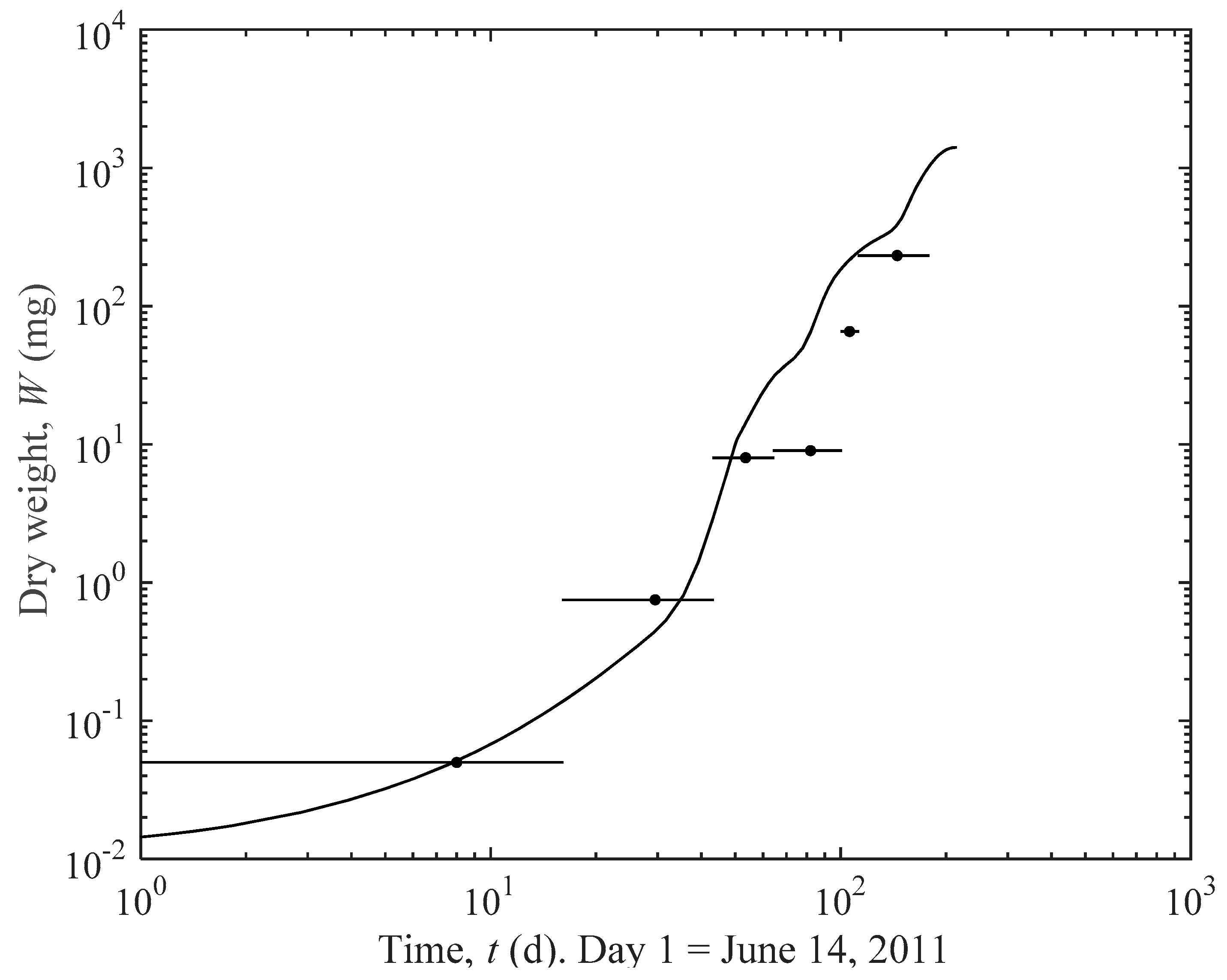
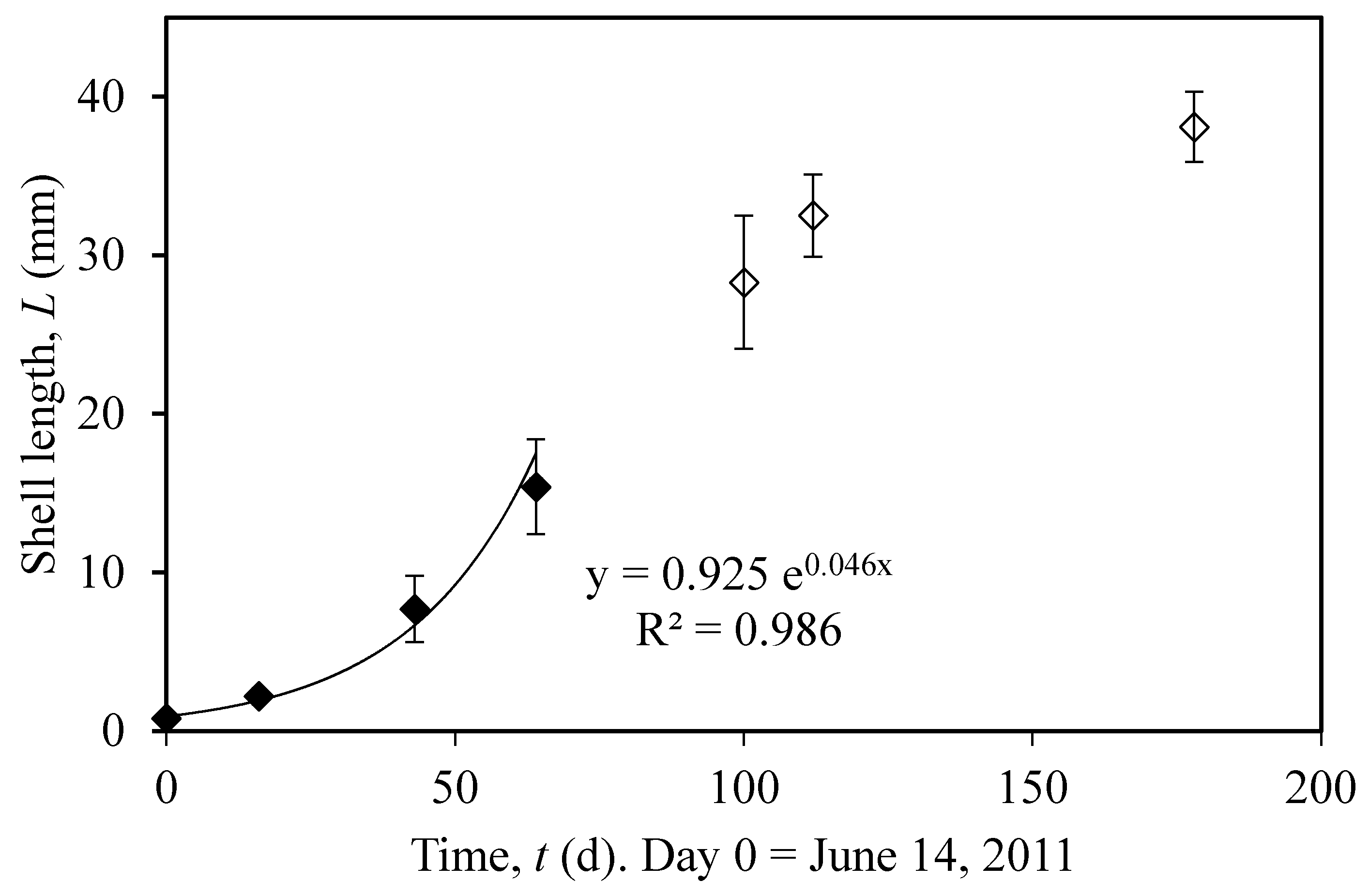
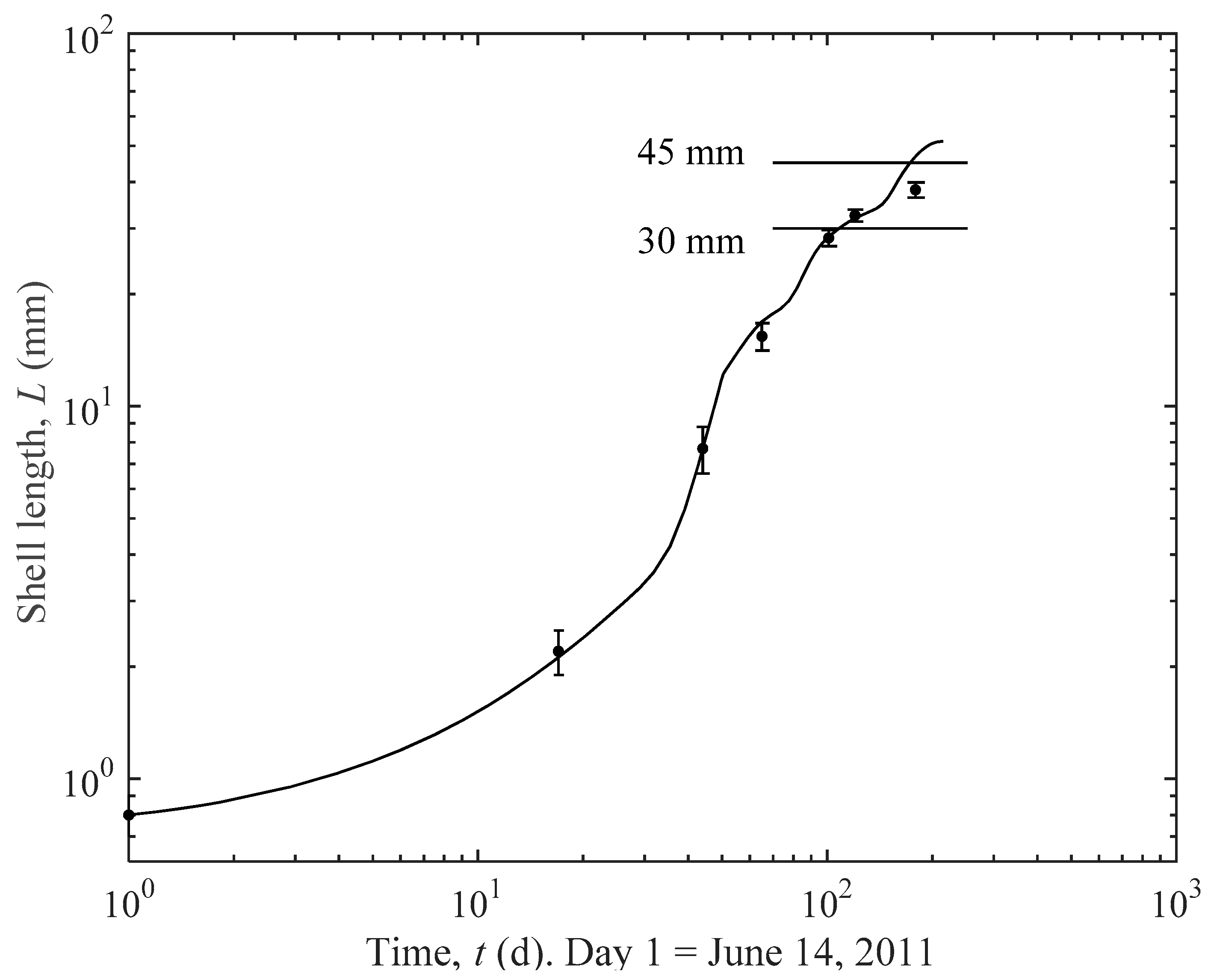
3.1. Actual and Predicted Growth of Mussels, from Newly Settled to Mini-Mussel

First, using the extended model, Equation (2) for small mussels, and the BEG model, Equation (5) for large mussels, accounting for time histories C(t) and T(t) from Figure 2, and AE = 0.90, the numerical integration gives the growth curve W(t) shown in Figure 3 from which the corresponding growth curve L(t) in Figure 4 is calculated by the allometric relations, Equations (1) and (4). To use log-log plots we set start of growth to Day 1. The value AE = 0.9, rather than 0.8 originally suggested in Reference [3], is used because it provides improved predictions for the conditions in Great Belt [4].
According to Figure 4 the predicted growth is close to the recorded data and it is predicted that mussels should have reached the mini-mussel size of 30 mm shell length at Day 121 which corresponds to 13 October of 2011. Additionally, an initial size variation given by 0.8 ± 0.1 mm leads to only the small variation Day 121 ± 1 as the time to reach size 30 mm shell length. As mentioned mussels had reached a shell length of about 38 mm at Day 178 9 December at which time the model predicts 44.7 mm. This suggests that it is feasible to produce mini-mussels [2] in Great Belt during one season.
Second, for the ad hoc BEG model, using time histories C(t) and T(t) from Figure 2, and setting AE = 0.90, the governing Equations (5) and (11) for small and large mussels are integrated numerically to give the growth curve W(t) shown in Figure 5 from which the corresponding growth curve L(t) in Figure 6 is calculated by the allometric relations, Equations (1) and (4). According to Figure 6 the predicted growth is close to the recorded data and it is predicted that mussels should have reached the mini-mussel size of 30 mm shell length at Day 108 which corresponds to 30 September of 2011. Additionally, mussels had reached a shell length of about 38 mm at Day 178 9 December at which time the model predicts 47 mm. This suggests that it is feasible to produce mini-mussels [2] in Great Belt during one season and possibly also the usual marketable 45 mm mussels when feeding conditions are more favorable (i.e., > 2.5 µg chl a L−1).

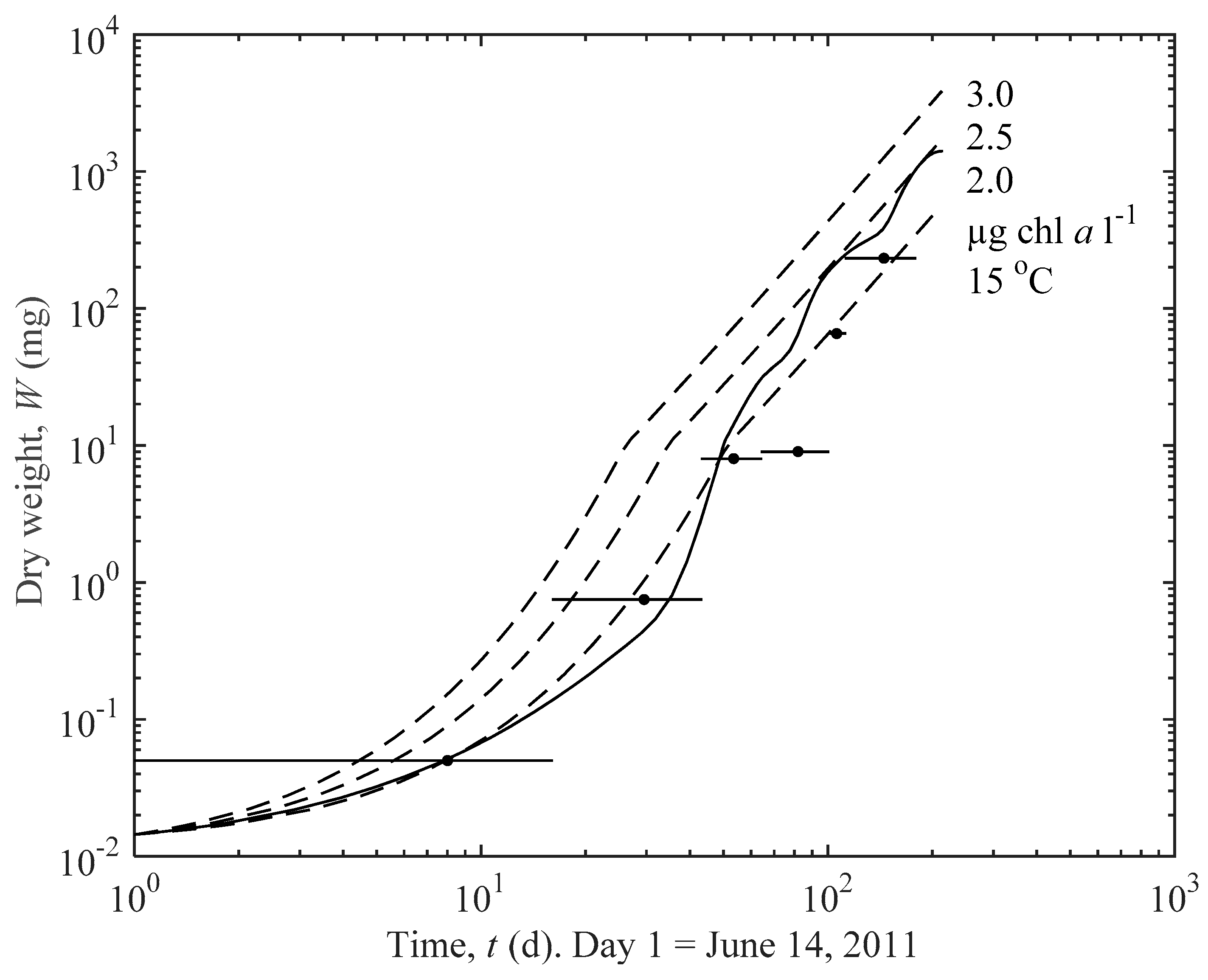
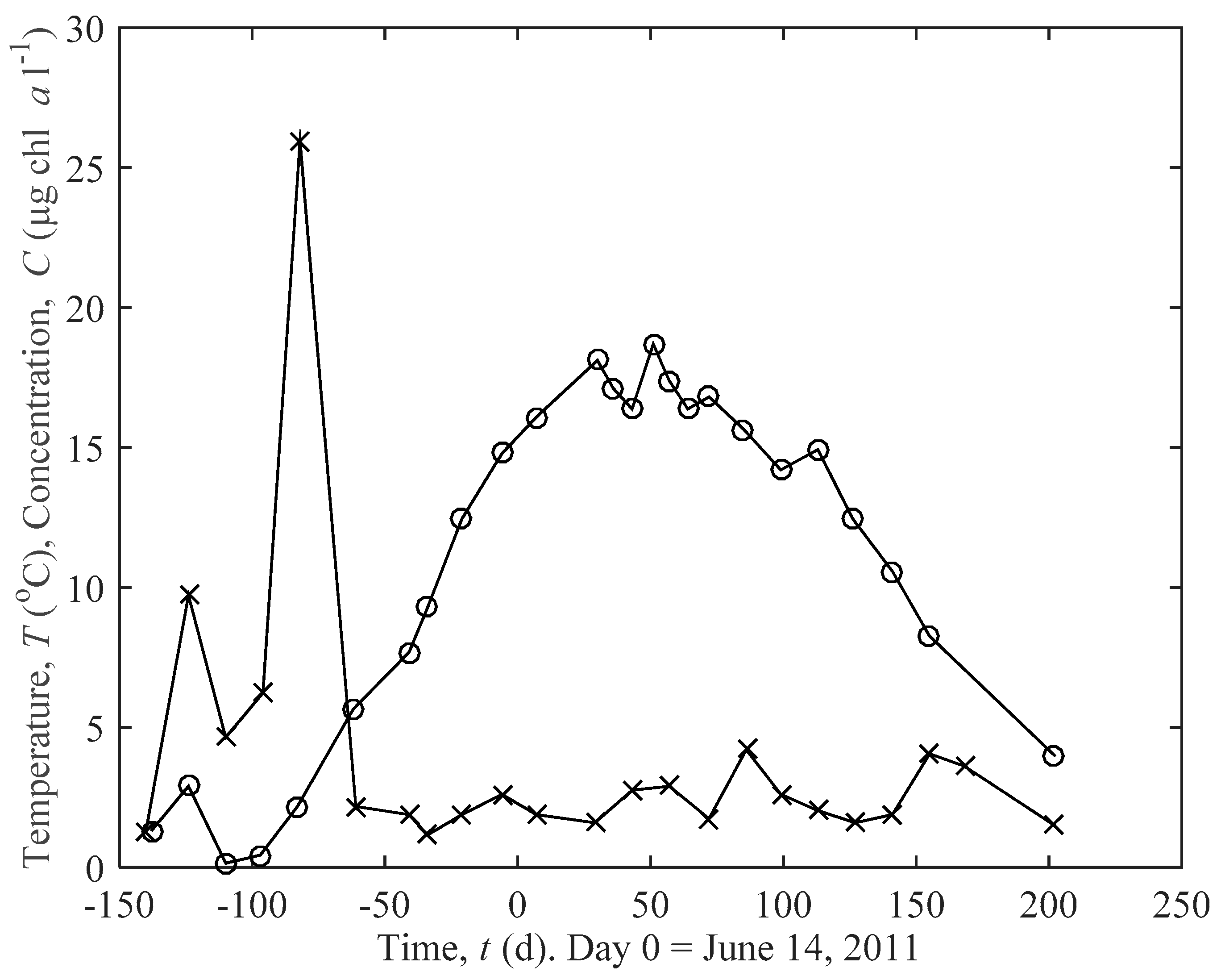
3.2. Predicted Influence of chl a and Temperature on Growth

As an illustration, for T = 15 °C and AE = 0.90, Figure 5 and Figure 6 (dashed curves) show the predicted growth of initially 0.8 mm shell length mussels for 3 constant values of chl a: 2, 2.5 and 3 µg·L−1, respectively. The time to reach 30 mm and 45 mm, respectively, are listed in Table 2. If growth started on 14 June the 30 mm shell size would only be reached during the remaining 201 days of the year 2011 provided C > 2 µg chl a L−1. Model predictions are quite sensitive to the chl a concentration which should, therefore, be recorded close to the production site. Although the distance of 12 km between monitoring station and mussel test site may have introduced some uncertainty we believe that the two locations have near identical chl a concentration due to the hydrography in Great Belt [2].
As another illustration, for AE = 0.90 and C = 2.5 µg chl a L−1, the model predictions lead to times for growth from size 0.8 to 30 mm shown in Table 2. These results indicate a fairly weak effect of temperature change in the range 5 to 15 °C and should be taken with some caution since the temperature dependence has not yet been included for small mussels.

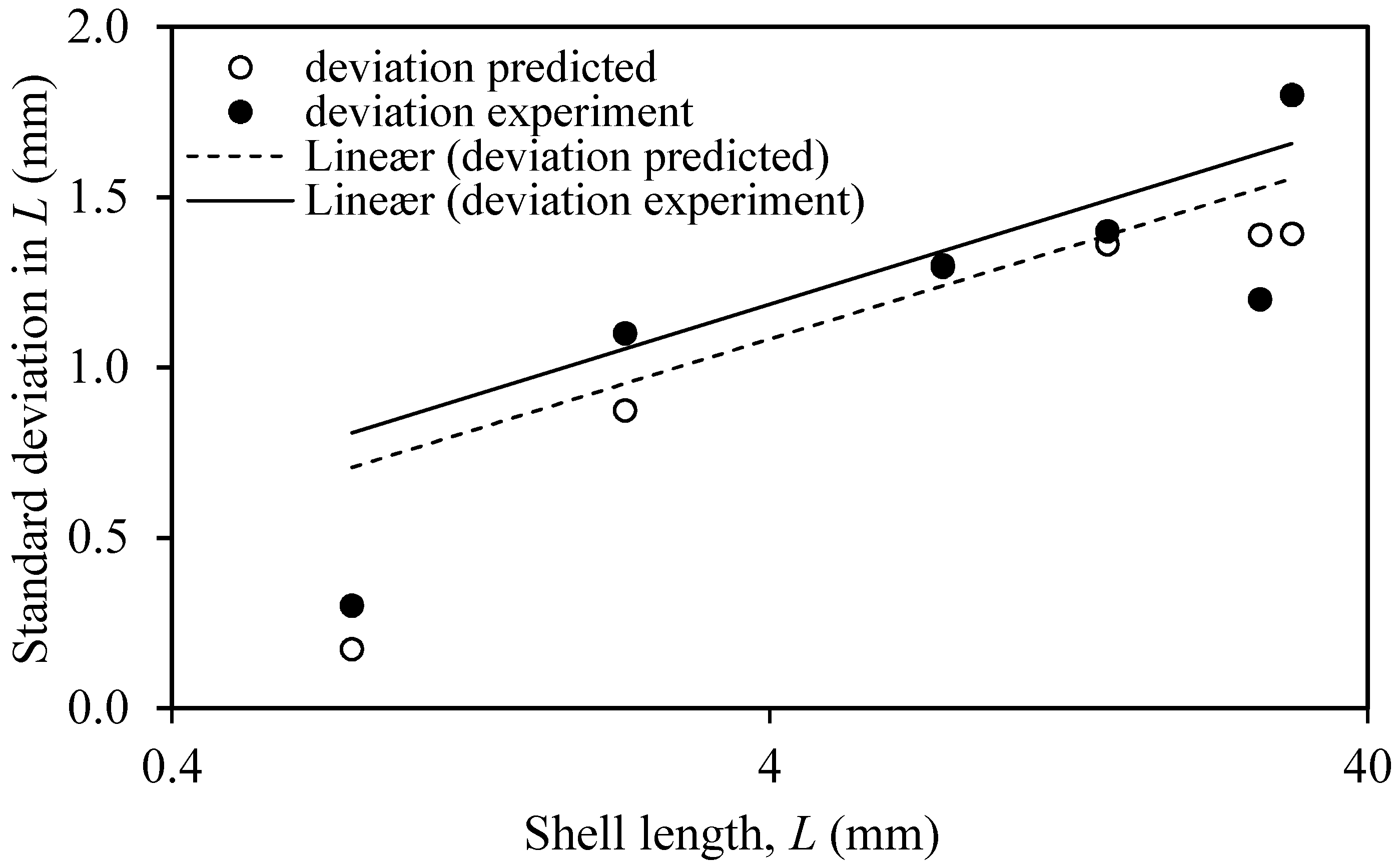
3.3. Sensitivity to Change of Model Exponents

Integrating the model equations from the nominal initial 0.8 mm shell length with a change of both exponents 0.866 = 1 − 0.134 in Equation (2) and 0.66 = 1 − 0.34 in Equation (5) by ±1% leads to predicted deviations that are compared to experimental values of standard deviations in Figure 7. Despite the considerable scatter of the limited data the general trend and magnitude of results are close as indicated by the linear regressions lines.

4. Discussion

The present growth model is based on the previously developed and tested modified BEG model Equation (5) for juvenile mussels (of shell length > about 10 mm), supplemented either by the extended model Equation (2) or by the ad hoc BEG model Equation (11), both developed for small post-metamorphic mussels (of shell length < about 10 mm). These new models are tested here for the first time. They are only based on the initial condition of initial mussel size at the start of integration supplemented by the time-varying environmental parameters of chl a concentration C(t) and temperature T(t) as integration proceeds, and neither model needs any other calibration or ‘forcing’.
For lack of more data on growth, filtration rate, and respiration for small post-metamorphic mussels the proposed ad hoc BEG model is somewhat speculative at this point for several reasons: (1) it is unknown if, as assumed in the scaling leading to Equation (11), the ratio of assimilated energy intake to maintenance respiration is the same for small and large mussels and that these terms follow power laws with the same exponent of W; (2) the metabolic cost of growth (i.e., synthesis of new biomass) may be higher in small than in large mussels where the cost of growth constitutes an amount of energy equivalent to 12% of the growth (biomass production) which was used in the original BEG model (Equation (5) in [3]); (3) the rejection of otherwise consistent data F(W) ≈ W1.03 and Rm(W) ≈ W1.14 from [6] showing 2 different exponents > 1 in favor of Rm(W) ≈ W0.887 from [7] in Equation (10) in anticipation of an exponent < 1. The latter choice has been based on the trend of the specific growth rate µ(W) ≈ W−0.134 or, as given in Equation (2) G(W) ≈ W0.866, of the only available field data for growth of this size class of mussels. Additionally noted in Reference [7] is the monotonous change of exponents b in Rm(W) ≈ Wb from veliger larvae [8] (b = 0.903), over post-metamorphic (b = 0.887) to juvenile and adult (b = 0.663) mussels. For an overview of equations and conversion factors used in relation to development of the various BEG models, see Table A1 in Appendix A.

4.1. Prediction Estimates

As shown earlier for the larger mussels (Figure 9 of [4]) the BEG model responds significantly to the environmental parameters of chl a and temperature and more so than some other models tested for the prediction of mussel growth in temperate Danish waters, such as SFG and DEB. This is also reflected for the present prediction in Figure 4 and more so in Figure 6, cf. Table 2. But for the smaller mussels it remains to include the influence of temperature which awaits more data. It should be stressed that the results in Figure 4 and Figure 6 do not represent an objective validation of the extended BEG models but constitute a step of further model development and illustrations of schemes to reach the objective of the present study. Actual validation awaits more data on the early growth of mussels. In the long run such an effort may lead to the development of useful graphs for planning and managing aquacultures.
The good agreement between predictions and data for the smaller mussels is not surprising since Equation (2) was derived from these data and Equation (11) was scaled to match the coefficient 4.248 of Equation (2). Yet the integration over the extended period of nearly 200 days with a 4½ decade change in dry weight is a challenge well handled by the models. The mean values of ambient parameters from Figure 2 during the early growth period was 2.47 µg L−1 and 14.6 °C which are close to those of the data points (2.4 µg chl a L−1 and 16.9 °C on the average) although there were periods of less than 2 µg chl a L−1 which appear to show up in Figure 6 as slower growth form Day 10 to 30. The rather high growth rate near the end of the period may be ascribed to the high chl a concentrations shown in Figure 2 (up to 4 µg·L−1) and despite the decreasing temperature which has a lesser effect on growth. Although the heterotrophic fraction of the total plankton biomass in Great Belt (amounting to 3.4% in 1997, [2]) is also available for filter-feeding mussels the autotrophic plankton, quantified by the chl a concentration, dominates the ingested food. This could justify use of the higher value AE = 0.9 (in place of the standard value 0.8) as was done by [4] in comparing various models to other growth data. In that case a shell size of 30 mm is predicted to be reached at Day 121 instead of Day 148, suggesting a likely uncertainty in the predictions.
It is also noted that the present model predictions apply to environmental conditions where the mussels are fully open and continuously exploiting their filtration capacity [3]. A study [9] showed that the functional response of Mytilus edulis resembles a Type I in terms of ingestion, but with a rapid decrease instead of a constant above the limit of incipient saturation concentration of about 8 µg chl a L−1 [10]. The physiological implications of the functional response remain uncertain [11], but a survey of naturally occurring chl a concentrations in the sea shows that these are generally below the limit of incipient saturation concentration [9]. Therefore, it may be suggested that M. edulis generally filter at maximum rates as long as the chl a concentration exceeds the minimal concentration of about 0.5 to 0.9 µg chl a L−1 below which the mussels close their valves and reduce or cease filtering [12]. The last-mentioned closing phenomenon may frequently occur in dense mussel beds [13], but probably not in adequately thinned suspended farm-rope cultures.

4.2. Importance of Thinning for Optimal Growth

Newly reported observations show that mussel larvae are omnipresent in the Great Belt and other Danish waters and that the larval density is sufficient for recruitment to future line-mussel farms [14]. In dense populations of mussels on cultivation ropes, increases in size of individuals and the resulting increment of their requirements for space and food cause intraspecific competition and result in decreased growth rates and increased mortality [15,16,17,18]. Such aspects are not included in the present growth model which has shown fairly good agreement with the growth of the group of larger mussels because these mussels have supposedly been situated favorably on ropes to attain their larger size as compared to the mean of all mussels. The ability of small mussels to move (by means of their foot) to areas of the farm-rope, which may have been mechanically cleaned by a brushing machine, should in future studies be examined for different sizes of mussels during the growth season. Additional studies should consider the behavior and growth of newly settled and small mussels in controlled laboratory experiments in order to determine the optimal density of mussels on farm-ropes. Further, important knowledge about the effect of thinning on optimal growth may be obtained through regular sampling of mussels to determine their spatial distribution on the farm-rope and their actual growth rate. Likewise, regular measurement of temperature and the ambient chl a concentration combined with use of the present growth model may significantly increase our understanding of the effect of intraspecific competition in order to identify the optimal mussel density and provide a basis for a rational mechanical thinning.
The growth of shell length shown in Figure 1 is suggested to represent the maximum possible at the actual chl a concentration because only the outermost 10 biggest mussels in samples from farm-ropes were used for calculating the mean shell length; but the many much smaller mussels (up to 290 ind. cm−1 rope in mid-July 2011) in the samples indicate a high degree of intraspecific competition between the remaining densely packed mussels sitting close to the farm-rope. While the larger group 3 mussels examined here reached a mean shell length of 38.1 mm at the end of the study the mean of all mussels on the densely populated ropes reached only 46% of this length (Figure 4 of [5]) which clearly reflects the competition. A recent study of juvenile mussels on densely populated pieces of ropes [19] showed that re-filtration of water resulted in lower clearance rates compared to maximum filtration rates as used in the present model. Extrapolating maximum filtration rates to estimate the ingestion rates of dense populations of mussels may thus lead to an overestimation of the actual food-energy uptake. This emphasizes the need of thinning to optimize the individual growth by eliminating the intraspecific competition and it also justifies (although we are not able to specify more precisely how this may technically be done) that we compare the predicted with the actual growth of the outermost 10 biggest mussels that have probably not been impeded by competition (re-filtration), but realized their full filtration capacity as presupposed by the prediction model which is relatively simple and easy to use. Therefore—although the present model does not include effects such as mortality or spawning as do more elaborate models, e.g., [20,21]—it may in the future be used as a practical instrument to evaluate to what degree the actual growth of line-mussels in the field deviate from the potential (optimal) growth under specified chl a and temperature conditions.
Finally, an overlooked aspect of thinning seems to be the ability of mussels to actively clean own shells by the foot (and prevent fouling by algae or epifauna, e.g., barnacles [22]). Especially young mussels have usually clean and smooth shells, but on densely populated mussel-ropes this ability may be hampered due to lack of space. Therefore the ability of small mussels to both spread to cleaned areas on the farm-rope and to keep their own shells clean is an important factor for realizing the growth potential at given temperatures and chl a concentrations as described by the present model.

Acknowledgments

This work formed part of the MarBioShell project (2008-2012) supported by the Danish Agency for Science, Technology and Innovation. Thanks are due to two anonymous reviewers for constructive comments to the manuscript.

Author Contributions

P.S.L. and H.U.R. contributed equally to model development and paper writing; P.S.L. did calculations and data analysis; H.U.R. designed and executed experiments.

Conflicts of Interest

The authors declare no conflict of interest.

Abbreviations

The following abbreviations are used in this manuscript:
BEG
BioEnergetic Growth model

Appendix A

The following Table A1 gives correlations from the literature for 3 size ranges of Mytilus edulis:
  • Veliger larvae
  • Young post-metamorphic mussels
  • Juvenile and adult mussels
The available basic correlations include:
  • Allometry, W(L)
  • Filtration rate, F(W)
  • Respiration, R(W)
where
  • F = filtration rate (clearance)
  • L = shell length
  • Rm = maintenance respiration
  • W = dry weight of soft parts
with appropriate units given after variables in the equations.
Derived BEG models involve the variables:
  • a0 = 1.12 (factor accounting for cost of growth, assumed = 0.12 × G)
  • AE = assimilation efficiency
  • C = algal concentration expressed as chlorophyll (chl a)
  • G = dW/dt = growth rate
  • NGE = net growth efficiency
  • t = time
  • µ = W−1dW/dt = specific growth rate.
Table A1. Correlations and equations used in the development of BEG prediction models.
Eq.CorrelationCorrelation (Alternative Units)°CReference
I. Veliger larvae (10−8–10−6 g)
1W(µg) = 2.53 × 10⁻⁹ L(µm)3.49W(mg) = 0.0747 × L(mm)3.4912[23]
2F(µL·h−1) = 1.25 × 10⁻⁵ L(µm)2.85F(µL h−1) = 132 × W(µg)0.81717–19[23]
3 F(L h−1) = 10.5 × W(g)0.817
4Rm(nL O2 h−1) = 3.10 × W(µg)0.902Rm(mL O2 h−1) = 0.801 × W(g)0.90315Figure 3 of [8]
Potential BEG-model based on Equations (3) and (4)
5G = dW/dt = (C × AE × FRm)/1.12
6G(%g·d−1) = 1.228 × C × (AE/0.8) × W(g)0.817 − 1.664 × W(g)0.902
7µ(% d−1) = 1.228 × C × (AE/0.8) × W(g)−0.183 − 1.664 × W(g)−0.098
Estimate based on NGE = 2/3 and Equation (4); (NGE ~ 43%–73%)
8µ = NGE × R/[(1-NGE) × W][7]
9µ(d−1) = 0.0388 × W(g)−0.097 G(d−1) = 0.0388 × W(g)0.903cf. [24]
Estimate based on measured shell length L versus time t and Equation (1)15Figure 7 of [23]
10L(mm) = 0.0634 + 0.0087 × t(d) G(g·d−1) = 0.01254 × W(g)0.713
11µL(d−1) = 0.0087 × L(mm)−1 µ(d−1) = 0.01254 × W(g)−0.287
Other relations:
F(µL·h−1) = 220 × W(µg)0.846F(L·h−1) = 26.2 × W(g)0.84615Figure 2 of [8]
II. Young post-metamorphic mussels (10−6–10−2 g)
12W(mg) = 0.0247 × L(mm)2.42see also [5] (Figure 8)12[23]
13F(mL·h−1) = 0.025 × W(µg)1.03F(L h−1) = 37.84 × W(g)1.0312–14Figure 4 of [6]
14Rm(nL O2 h−1) = 0.287 W(µg)1.14Rm(mL O2 h−1) = 0.1986 × W(g)1.1412–14Figure 6 of [6]
Potential BEG-model based on Equations (13) and (14)
15G = dW/dt = (C × AE × FRm)/1.12
16G(%g·d−1) = 4.424 × C × (AE/0.8) × W(g)1.03 − 0.413 × W(g)1.14
17µ(% d−1) = 4.424 × C × (AE/0.8) × W(g)0.03 − 0.413 × W(g)0.14
18Rm(µL O2 h−1) = 315 × W(g)0.887Rm(mL O2 h−1) = 0.315 × W(g)0.88712Figure 1 of [7]
Extended BEG-modelBased on field data Figure 5 of [5]
19G(mg·d−1) = 4.248 × W(mg)0.866µ(% d−1) = 4.248 × W(g)−0.134Present
Ad hoc BEG-model based on Equations (18) and (19) and scaling of Equation (25)
20G(%g·d−1) = [4.89 × C × (AE/0.8) − 5.54] × W(g)0.887Present
III. Juvenile and adult mussels (10−2–1 g)
21W(mg) = 0.00215 L(mm)3.40 Figure 8 of [5]
22F(L h−1) = 7.45 × W(g)0.66 10–13Equation (8) of [3]
23Rm(µL O2 h−1) = 475 × W(g)0.663Rm(mL O2 h−1) = 0.475 × W(g)0.66314Figure 1 of [7]
Basic BEG-model based on Equations (23) and (24)
24G = dW/dt = (C × AE × FRm)/1.12[25]
25G(%g·d−1) = 0.871 × C × (AE/0.8) × W(g)0.663 − 0.986 × W(g)0.66[3]
26µ(% d−1) = 0.871 × C × (AE/0.8) × W(g)−0.34 − 0.986 × W(g)−0.34
27Modified BEG-model: G(mg·d−1) = C1 × W(mg)0.66 Equation (5) of [4]
28C1 = 0.1047 × m1 × (0.871 × m2 × n2 × C × AE/0.80 − 0.986 × m3 × n3)
29m1 = 1.12/[1 + (a0 − 1)n3 (1 − E)]; m2 = 1 − E; m3 = 1 − 0.9(1 + C/C0)E;
30E = exp(−C/C0); C0 = 0.4 µg chl a l−1; n2 = [1 + 0.0251(TTF)];
31n3 = 1.54(TTQ)/10; TF = 11.5 °C; TQ = 14 °C

References

  1. Dolmer, P.; Frandsen, R.P. Evaluation of the Danish mussel fishery: Suggestions for an ecosystem management approach. Helgol. Mar. Res. 2002, 56, 13–20. [Google Scholar] [CrossRef]
  2. Riisgård, H.U.; Lundgreen, K.; Larsen, P.S. Potential for production of ‘mini-mussels’ in Great Belt (Denmark) evaluated on basis of actual growth of young mussels Mytilus edulis. Aquacult. Int. 2014, 22, 859–885. [Google Scholar] [CrossRef]
  3. Riisgård, H.U.; Lundgreen, K.; Larsen, P.S. Field data and growth model for mussels Mytilus edulis in Danish waters. Mar. Biol. Res. 2012, 8, 683–700. [Google Scholar] [CrossRef]
  4. Larsen, P.S.; Filgueira, R.; Riisgård, H.U. Somatic growth of mussels Mytilus edulis in field studies compared to predictions using BEG, DEB, and SFG models. J. Sea Res. 2014, 88, 100–108. [Google Scholar] [CrossRef]
  5. Larsen, P.S.; Lundgreen, K.; Riisgård, H.U. Bioenergetic model predictions of actual growth and allometric transitions during ontogeny of juvenile blue mussels Mytilus edulis. In Mussels: Ecology, Life Habits and Control; Nowak, J., Kozlowski, M., Eds.; Nova Science Publishers, Inc.: New York, NY, USA, 2013; pp. 101–122. [Google Scholar]
  6. Riisgård, H.U.; Randløv, A.; Kristensen, P.S. Rates of water processing, oxygen consumption and efficiency of particle retention in veligers and young post-metamorphic Mytilus edulis. Ophelia 1980, 19, 37–47. [Google Scholar] [CrossRef]
  7. Hamburger, K.; Møhlenberg, F.; Randløv, A.; Riisgård, H.U. Size, oxygen consumption and growth in the mussel Mytilus edulis. Mar. Biol. 1983, 75, 303–306. [Google Scholar] [CrossRef]
  8. Riisgård, H.U.; Randløv, A.; Hamburger, K. Oxygen consumption and clearance as a function of size in Mytilus edulis L. veliger larvae. Ophelia 1981, 20, 179–183. [Google Scholar] [CrossRef]
  9. Riisgård, H.U.; Pleissner, D.; Lundgreen, K.; Larsen, P.S. Growth of mussels Mytilus edulis at algal (Rhodomonas salina) concentrations below and above saturation levels for reducted filtration rate. Mar. Biol. Res. 2013, 9, 1005–1017. [Google Scholar] [CrossRef]
  10. Pleissner, D.; Lundgreen, K.; Lüskow, F.; Riisgård, H.U. Fluorometer controlled apparatus designed for long-term algal-feeding experiments and environmental effect studies with mussels. J. Mar. Biol. 2013. [Google Scholar] [CrossRef]
  11. Fréchette, M.; Urquiza, J.M.; Daigle, G.; Rioux-Gagnon, D. Clearance rate regulation in mussels: Adding the effect of seston level to a model of internal state-based regulation. J. Exp. Mar. Biol. Ecol. 2016, 475, 1–10. [Google Scholar] [CrossRef]
  12. Riisgård, H.U.; Egede, P.P.; Saavedra, I.B. Feeding behaviour of mussels, Mytilus edulis, with a mini-review of current knowledge. Mar. Res. 2011, 13. [Google Scholar] [CrossRef]
  13. Riisgård, H.U.; Larsen, P.S. Physiologically regulated valve-closure makes mussels long-term starvation survivors: test of hypothesis. J. Mollus. Stud. 2015, 81, 303–307. [Google Scholar] [CrossRef]
  14. Riisgård, H.U.; Lundgreen, K.; Pleissner, D. Environmental factors and seasonal variation in density of mussel larvae (Mytilus edulis) in Danish waters. Open J. Mar. Sci. 2015, 5, 280–289. [Google Scholar] [CrossRef]
  15. Alunno-Bruscia, M.; Petraitis, P.S.; Bourget, E.; Fréchette, M. Body size-density relationship for Mytilus edulis in an experimental food-regulated situation. Oikos 2000, 90, 28–42. [Google Scholar] [CrossRef]
  16. Filgueira, R.; Peteiro, L.G.; Labarta, U.; Fernández-Reiriz, M.J. The self-thinning rule applied to cultured populations in aggregate growth matrices. J. Mollus. Stud. 2008, 74, 415–418. [Google Scholar] [CrossRef]
  17. Lachance-Bernard, M.; Daigle, G.; Himmelman, J.H.; Fréchette, M. Biomass-density relationships and self-thinning of blue mussels (Mytilus spp.) reared on self-regulated longlines. Aquaculture 2010, 308, 34–43. [Google Scholar] [CrossRef]
  18. Cubillo, A.M.; Peteiro, L.G.; Fernández-Reiriz, M.J.; Labarta, U. Influence of stocking density on growth of mussels (Mytilus galloprovincialis) in suspended culture. Aquaculture 2012, 342–343, 103–111. [Google Scholar] [CrossRef] [Green Version]
  19. Jacobs, P.; Troost, K.; Riegman, R.; van der Meer, J. Length- and weight-dependent clearance rates of juvenile mussels (Mytilus edulis) on various planktonic prey items. Helgol. Mar. Res. 2015, 69, 101–112. [Google Scholar] [CrossRef]
  20. Bacher, C.; Gangnery, A. Use of dynamic energy budget and individual based models to simulate the dynamics of cultivated oyster populations. J. Sea Res. 2006, 56, 140–155. [Google Scholar] [CrossRef]
  21. Brigolin, D.; Maschio, G.D.; Rampazzo, F.; Giani, M.; Pastres, R. An individual-based population dynamic model for estimating biomass yield and nutrient fluxes through an off-shore mussel (Mytilus galloprovincialis) farm. Estuar. Coast. Shelf Sci. 2009, 82, 365–376. [Google Scholar] [CrossRef]
  22. Theisen, B. Shell cleaning and deposit feeding in Mytilus edulis L. (Bivalvia). Ophelia 1972, 10, 49–55. [Google Scholar] [CrossRef]
  23. Jespersen, H.; Karin Olsen, K. Bioenergetics in veliger larvae of Mytilus edulis L. Ophelia 1982, 21, 101–113. [Google Scholar] [CrossRef]
  24. Jørgensen, C.B. Growth efficiencies and factors controlling size in some mytilid bivalves, especially Mytilus edulis L.: Review and interpretation. Ophelia 1976, 15, 175–192. [Google Scholar] [CrossRef]
  25. Clausen, I.; Riisgård, H.U. Growth, filtration and respiration in the mussel Mytilus edulis: No regulation of the filter-pump to nutritional needs. Mar. Ecol. Prog. Ser. 1996, 141, 37–45. [Google Scholar] [CrossRef]
Figure 1. Mytilus edulis. Mean shell length of 10 biggest mussels in samples from farm-ropes in Great Belt in 2011 versus time [5], from newly settled 0.8 ± 0.1 mm post-metamorphic to 38.1 ± 1.8 mm mussels. Day 0 = 14 June 2011, Day 178 (last day) = 9 December 2011. The initial exponential increase in mean shell length, from 0.8 to 15.4 mm is indicated by closed symbols, the regression line and its equation.
Jmse 04 00042 g001
Figure 2. Temperature (○) and chl a concentration (×) recorded in Great Belt during 2011, Day 0 denoting 14 June at which the first newly settled mussels were observed. Data (Figure 2 from [5] replotted) from monitoring station (ST53; 55°30.46 N, 10°51.72 E) supplied by Environmental Centre Odense, Danish Ministry of the Environment. Mean (±S.D.) chl a concentration during 2011 after the bloom was 3.1 ± 2.1 µg chl a L−1.
Jmse 04 00042 g002
Figure 3. Mytilus edulis. Estimated growth history W(t) calculated from extended model Equations (2) and (5) for AE = 0.9 and the environmental conditions of temperature and chl a concentration given in Figure 2. Data (●) (Table 3 of [5]) representing average values over periods indicated by horizontal error bars.
Jmse 04 00042 g003
Figure 4. Mytilus edulis. Measured growth (●) with error bars from Figure 1 compared to calculated growth history L(t) from extended model Equations (2) and (5) for AE = 0.9 and the environmental conditions of temperature and chl a concentration given in Figure 2.
Jmse 04 00042 g004
Figure 5. Mytilus edulis. Estimated growth history W(t) calculated by ad hoc BEG-model, Equations (5) and (11) for AE = 0.9 and the environmental conditions of temperature and chl a concentration given in Figure 2. For comparison the predicted growth history at constant temperature (15 °C) and three values of chl a concentration (2, 2.5 and 3 µg·L−1) are shown (dashed). Data (●) (Table 3 of [5]) representing average values over periods indicated by horizontal error bars.
Jmse 04 00042 g005
Figure 6. Mytilus edulis. Measured growth (●) and error bars from Figure 1 compared to calculated growth history L(t) (solid) from ad hoc BEG-model, Equations (5) and (11) for AE = 0.9 and the environmental conditions of temperature and chl a concentration given in Figure 2. For comparison the predicted growth history at constant temperature (15 °C) and three values of chl a concentration (2, 2.5 and 3 µg·L−1) are shown (dashed).
Jmse 04 00042 g006
Figure 7. Mytilus edulis. Standard deviation from experiment (●) and model prediction (○) versus shell length, with corresponding linear regression lines (solid and dashed line, respectively). Standard deviation for predictions based on 1% deviation of exponents in growth equations.
Jmse 04 00042 g007
Table 1. Coefficients in Equation (6) [4].
m1 = 1.12/[1 + (a0 − 1)n3 (1 − E)]
m2 = 1 − E
m3 = 1 − 0.9(1 + C/C0)E
E = exp(−C/C0)
C0 = 0.4 µg chl a L−1
n2 = [1 + 0.0251(TTF)]
n3 = 1.54(TTQ)/10
TF = 11.5 °C; TQ = 14 °C
Table 2. Time (t) of mussel growth from 0.8 mm to 30 and 45 mm, respectively, at AE = 0.9, T = 15 °C and 3 values of constant chl a concentration (C), and time of growth to 30 mm at C = 2.5 µg chl a L−1 for 3 values of constant temperature (T). Based on ad hoc BEG model.
T = 15 °C
C (µg chl a L−1)22.53
t30 (d)15510580
t45 (d)249170129
C = 2.5 µg chl a L−1
T (°C)51015
t30 (d)115109105

