
The Influence of Bed Roughness on Turbulence: Cabras Lagoon, Sardinia, Italy


 and
and 
Abstract
:
1. Introduction

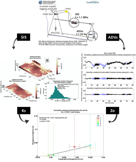
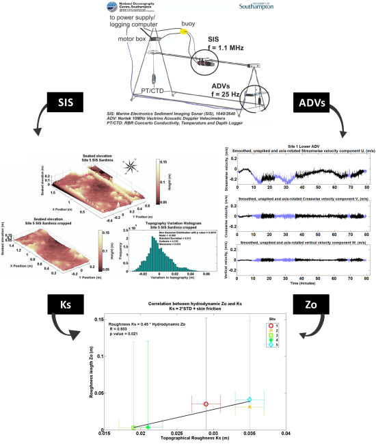
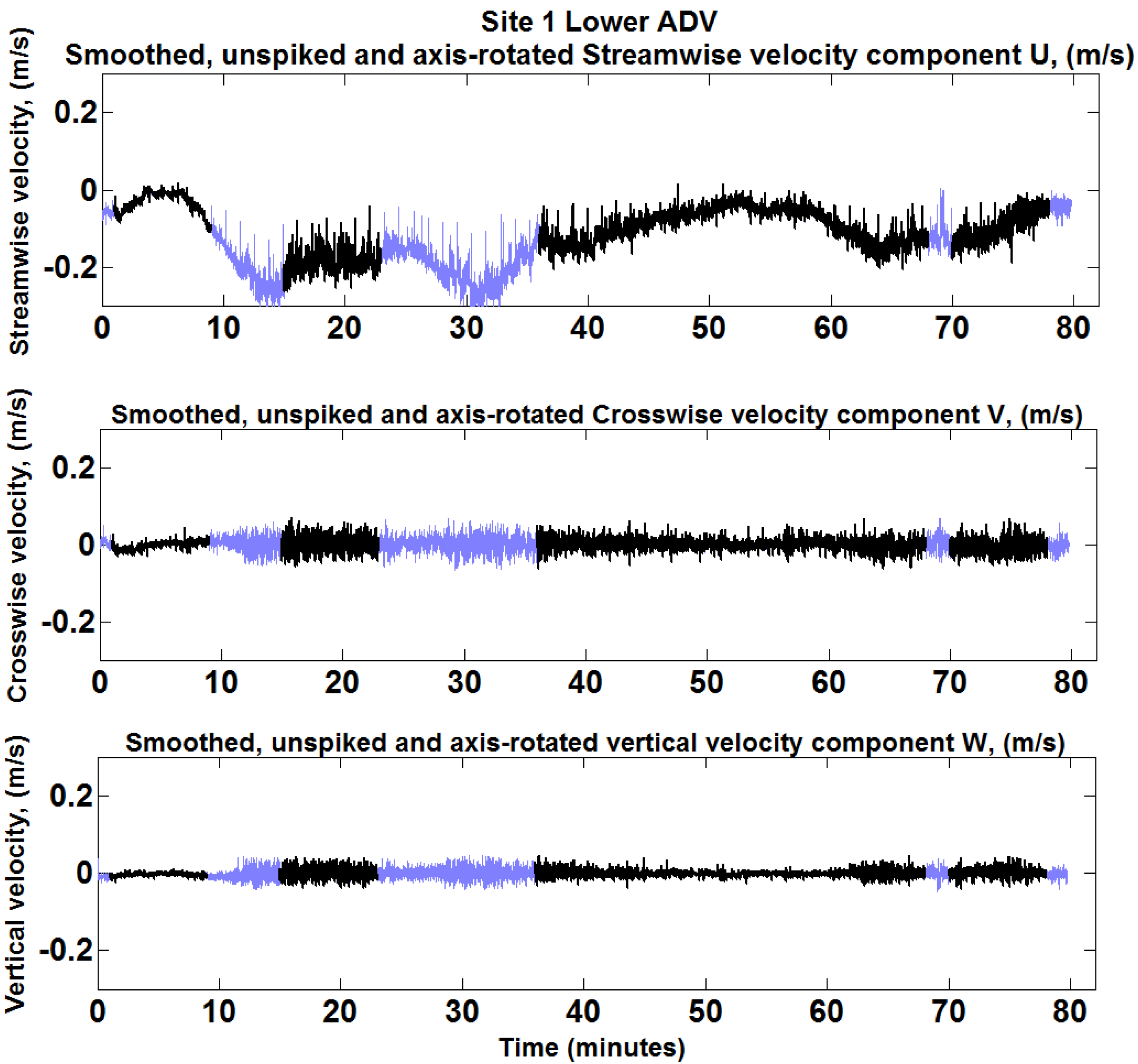
2. Methods
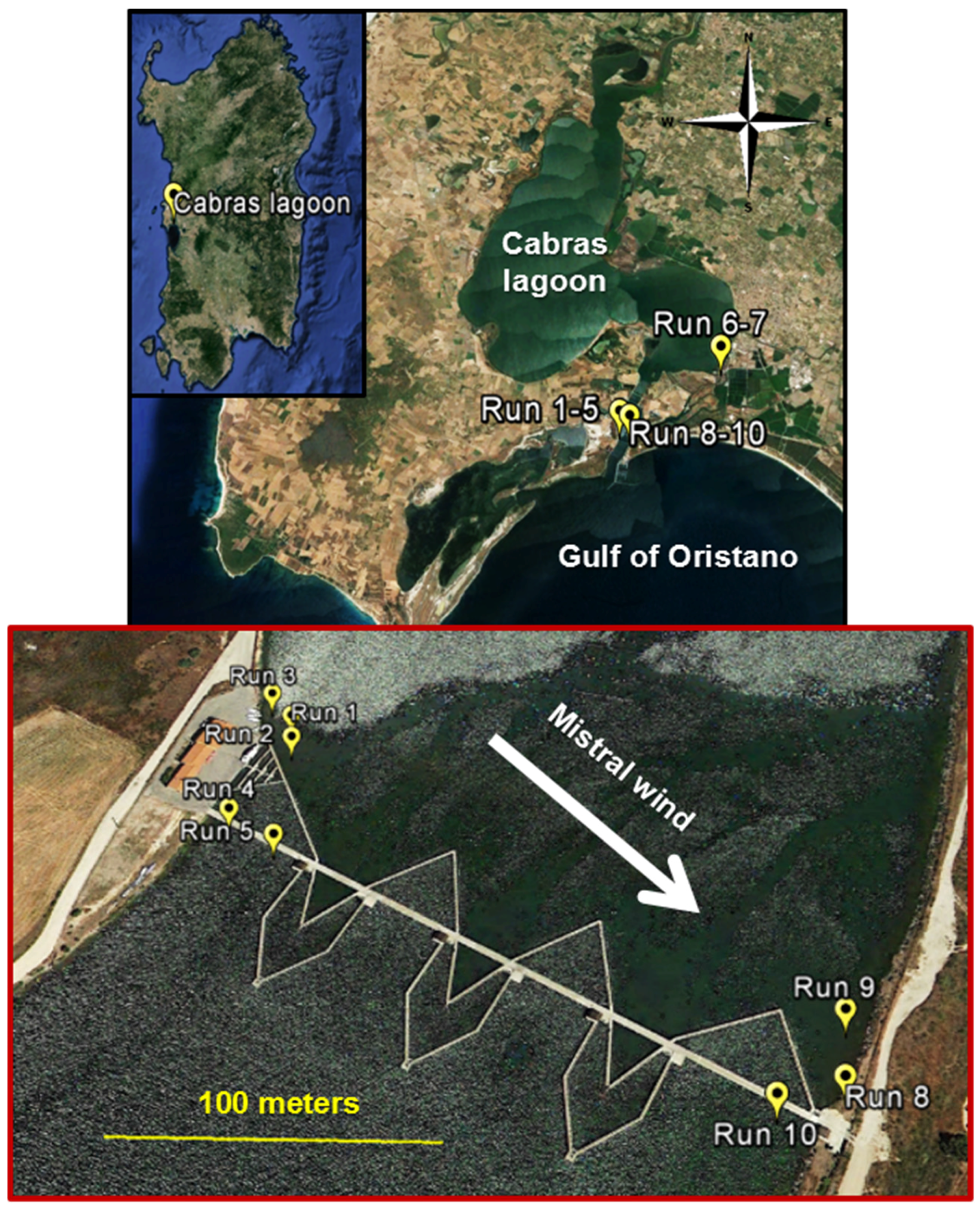
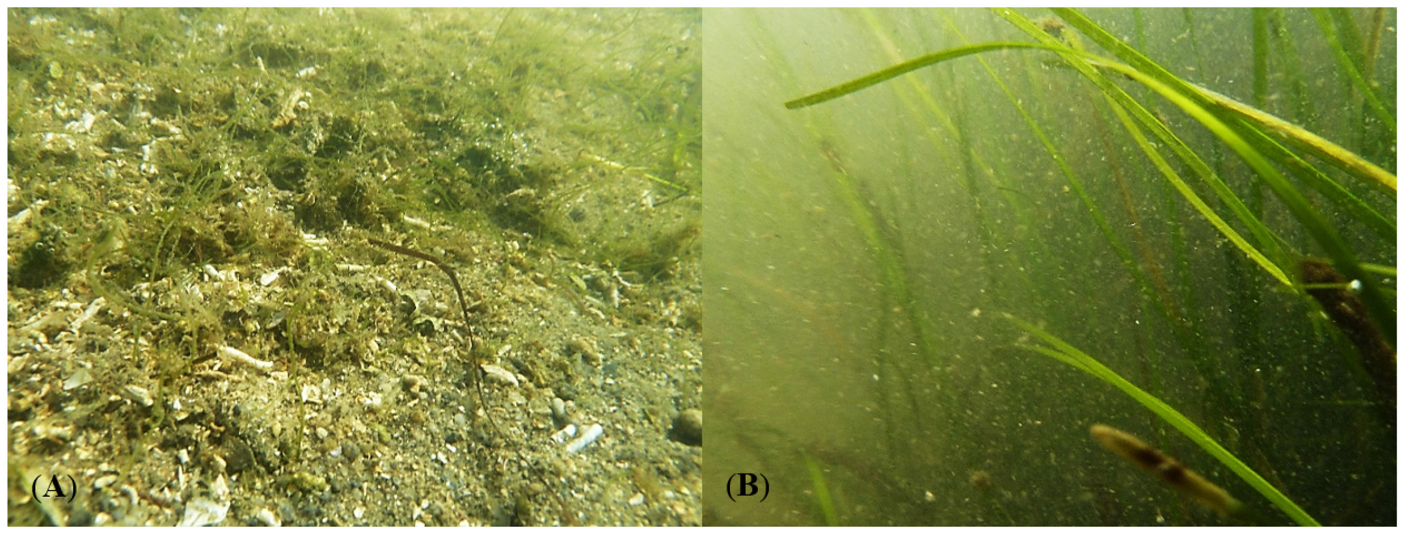
2.1. Study Site
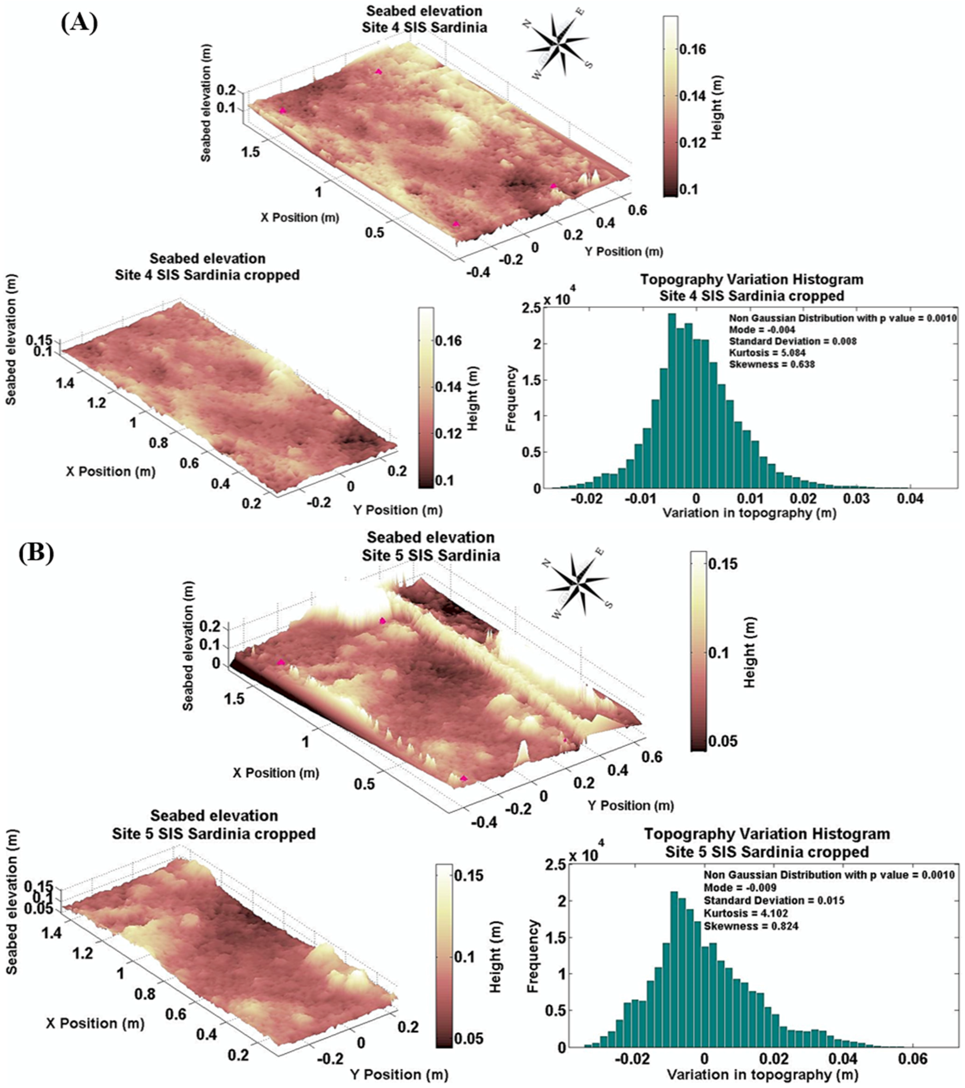
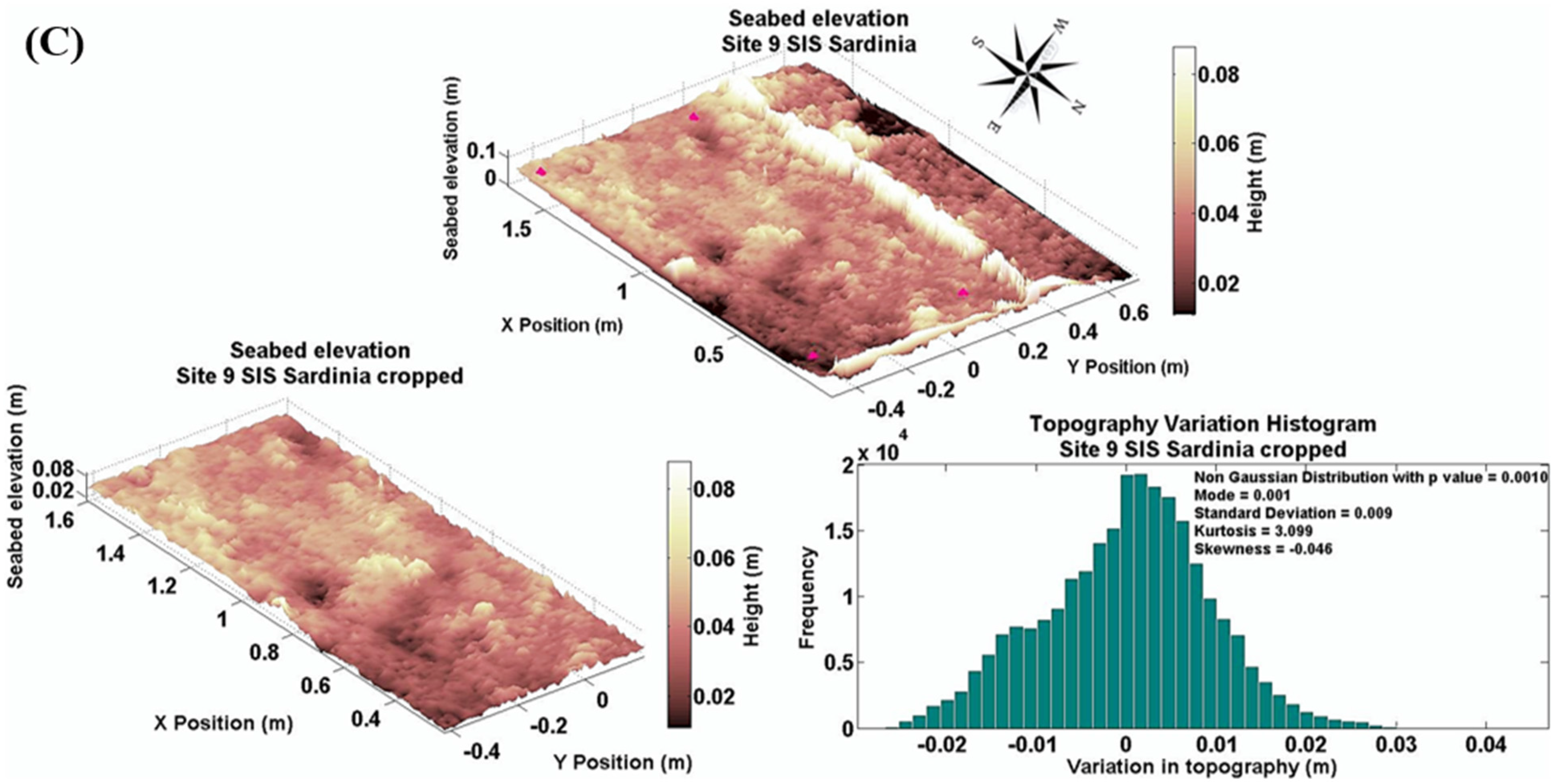
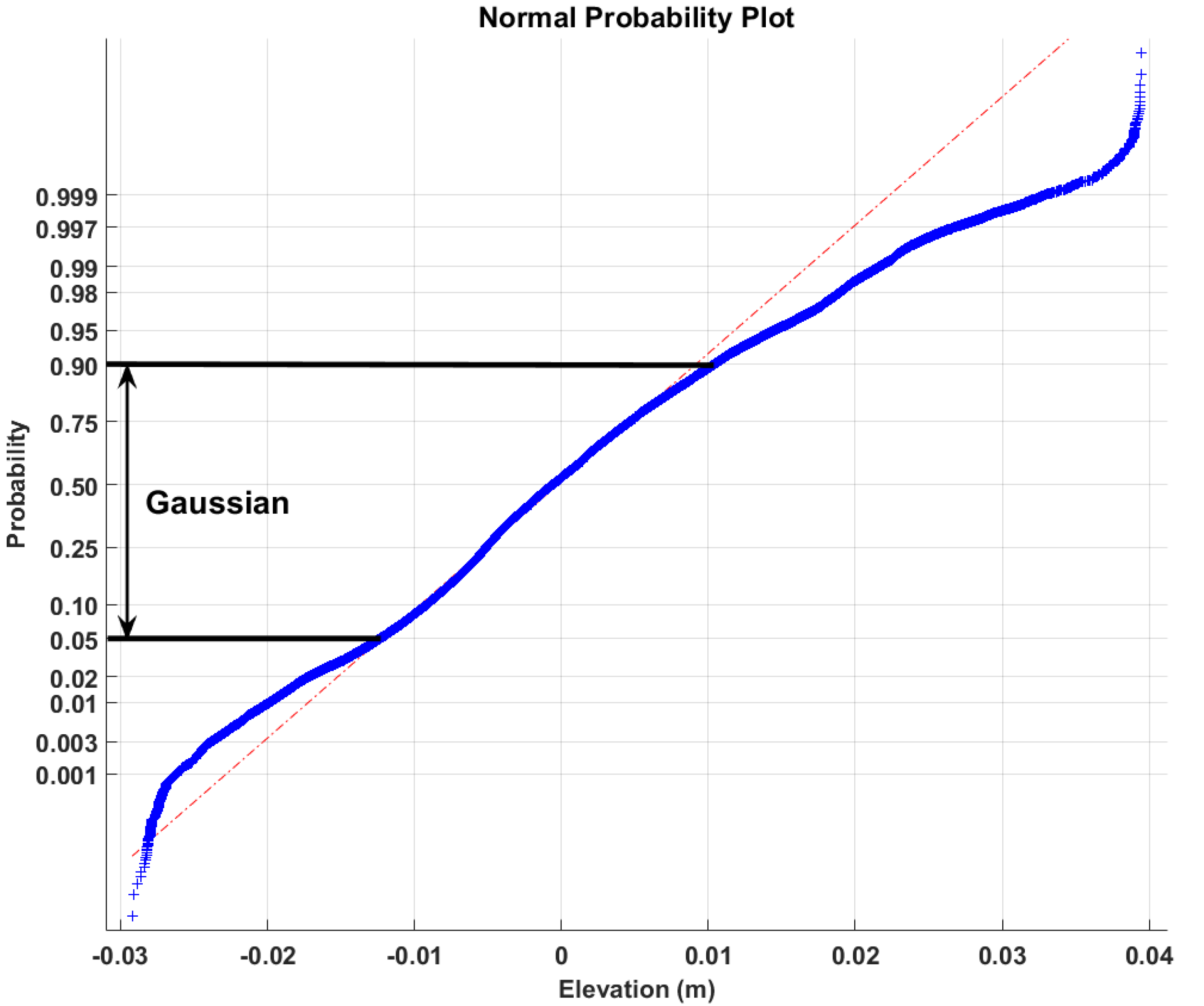
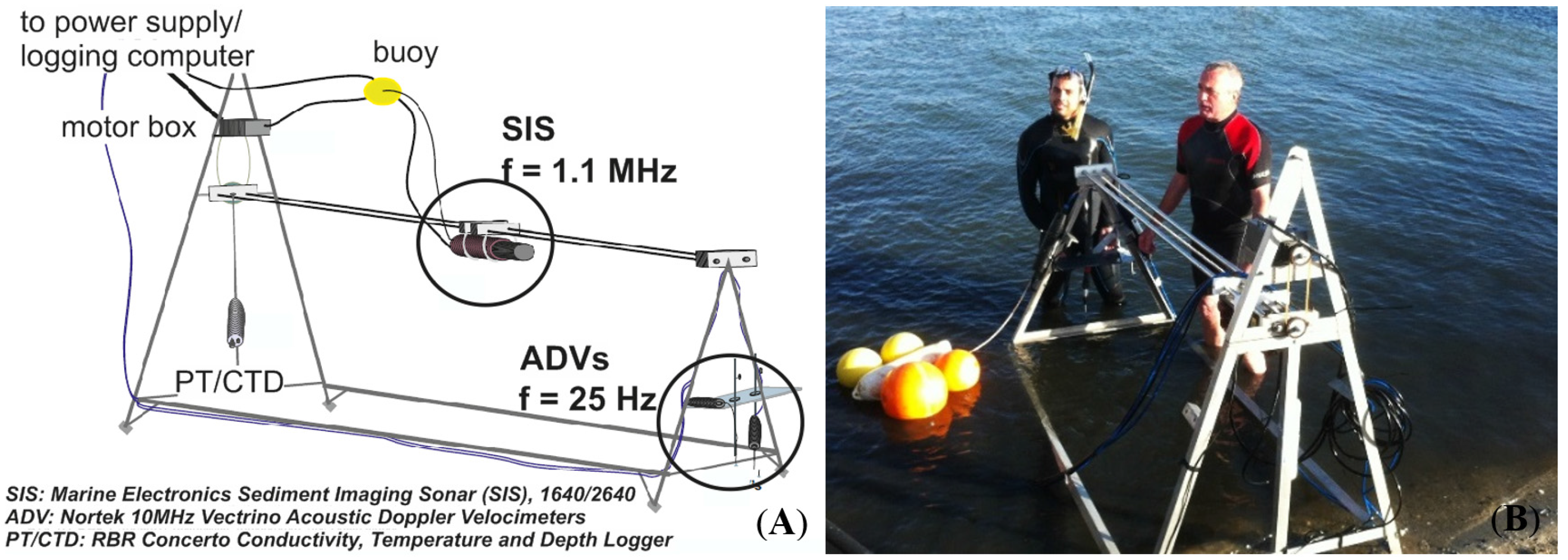
2.2. Topographical Bed Roughness Estimate Using BRAD


| Site | 1 | 2 | 3 | 4 | 5 | 6 | 7 | 8 | 9 | 10 |
|---|---|---|---|---|---|---|---|---|---|---|
| Latitude/Longitude | 39°54.594′; 8°29.532′ | 39°54.588′; 8°29.533′ | 39°54.600′; 8°29.526′ | 39°54.570′; 8°29.520′ | 39°54.564′; 8°29.532′ | 39°55.080′; 8°31.139′ | 39°55.106′; 8°31.181′ | 39°54.516′; 8°29.660′ | 39°54.528′; 8°29.663′ | 39°54.513′; 8°29.645′ |
| Water depth (m) | 1.06 | 1.28 | 1.22 | 1.36 | 1.54 | 1.36 | 1.02 | 1.01 | 0.94 | 1.16 |
| Wind speed (m/s) and direction | 5.3 NW | 7.2 NNW | 8.2 NW | 6.5 NNW | 8.5 NW | 8.2 NW | 8.2 NW; (gust speed 17.5) | 5.8 NW | 9.4 NW; (gust speed 15.9) | 10.1 NW; (gust speed 13.9) |
| Distance from inlet gate (>0 = N of weir) (m) | 5 | 4 | 20 | −7 | −4 | Not applicable | Not applicable | 6 | 24 | -6 |
| Height of the upper ADV (m) | 0.5 | 0.33 | 0.3 | 0.27 | 0.29 | 0.37 | 0.23 | 0.37 | 0.38 | 0.25 |
| Height of the lower ADV (m) | 0.32 | 0.14 | 0.01 | 0.011 | 0.17 | 0.2 | 0.05 | 0.18 | 0.08 | 0.08 |
| Sense of SIS scanning | South-North | North-South | South-North | South-North | South-North | North East-South West | South West-North East | South West-North East | North-South | North-South |
| State of the tide | Ebb | Low tide | Flood | Ebb | Flood (Flow inward, wind blowing from West) | Ebb (Current to South, gusts of wind from the North, rain) | Low tide (Strong continuous flow to South) | Ebb | Ebb: BRAD half exposed by end of run | Ebb (water level deeper to the West. Wind from South West) |
| Suspended sediment (g/L) | 0.01 | 0.04 | 0.03 | 0.01 | 0.02 | 0.04 | 0.06 | 0.06 | 0.03 | 0.08 |
| General description of seabed | Shelly mud. | Shelly mud. | Shelly mud. | Shelly mud. | Shelly mud with serpulid reefs. | Sandy gravelly bed over silt. High turbidity. Floating algae. Serpulid reefs. | High turbidity. Floating algae. Serpulid reefs up to 15cm high and 40cm long. | Shelly sand. Patches of seagrass. | Shelly, sandy mud. Seagrass cover. | Shelly mud. Seagrass, turbidity too high to determine its density. |

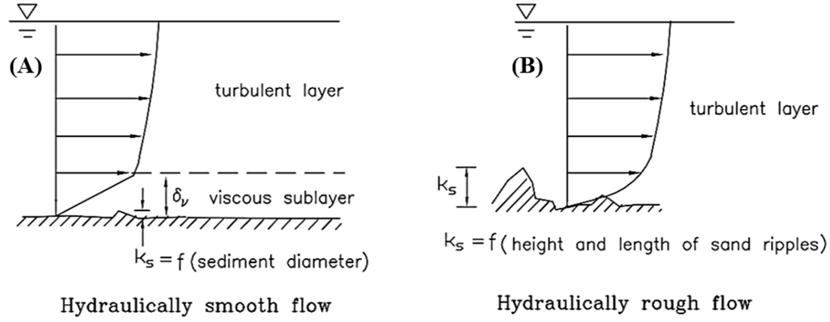
2.3. Roughness Length Zo Estimate

3. Results and Discussion
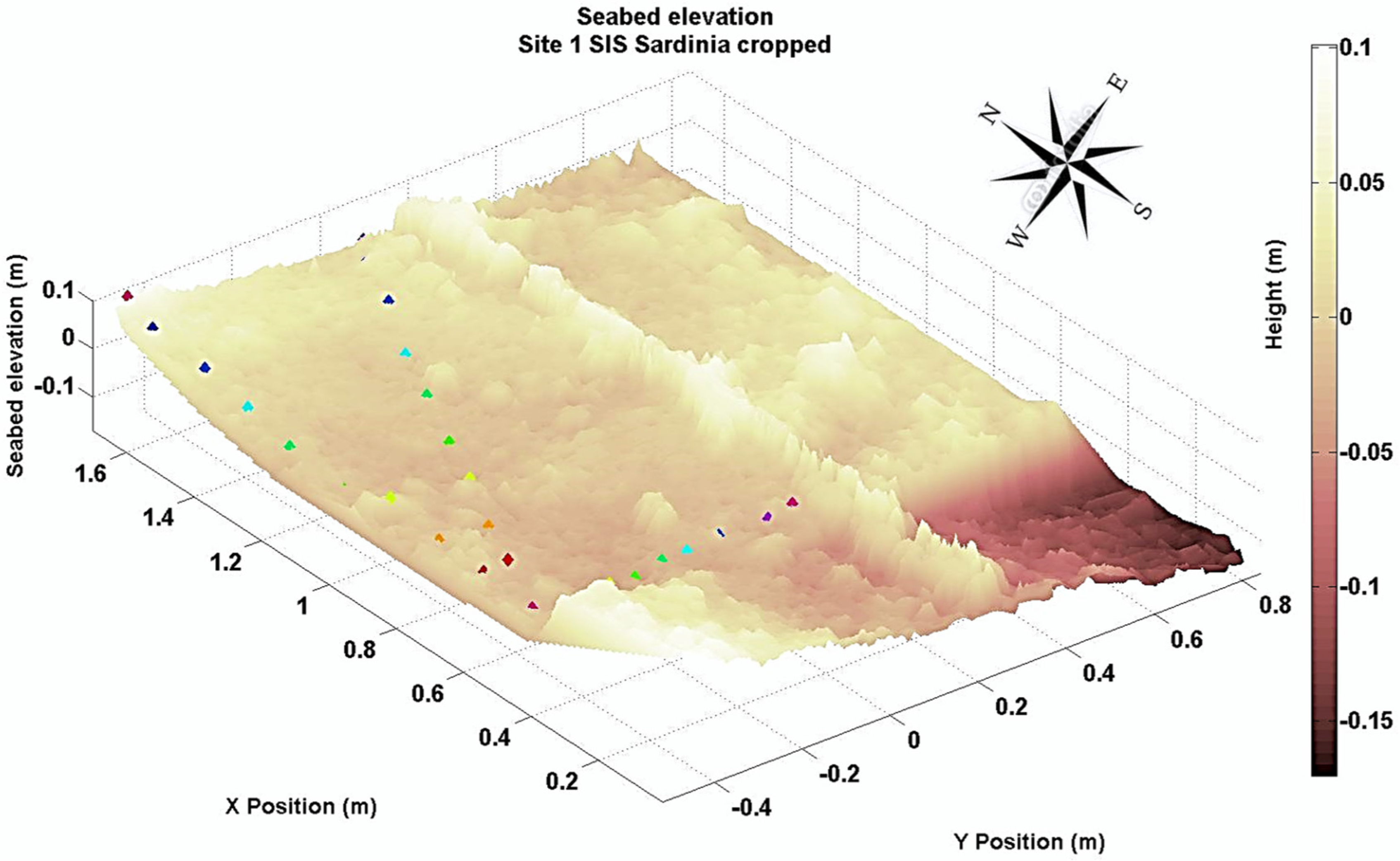
3.1. Characteristics of the BRAD Sites
| Site | Latitude/Longitude | Mean Velocity (m/s) | Standard Deviation of (m/s) | Turbulence U* (m/s) | Standard Deviation of U* (m/s) | Mean Zo (cm) | Standard Deviation of Seabed Elevation (cm) |
|---|---|---|---|---|---|---|---|
| 1 | 39°54.594′; 008°29.532′ | 0.118 | 0.018 | 0.008 | 0.004 | 3.52 | 1.4 |
| 2 | 39°54.588′; 008°29.533′ | 0.072 | 0.018 | 0.010 | 0.004 | 3.13 | 1.7 |
| 3 | 39°54.600′; 008°29.526′ | 0.053 | 0.012 | 0.007 | 0.003 | 0.32 | 0.8 |
| 4 | 39°54.570′; 008°29.520′ | 0.098 | 0.020 | 0.011 | 0.007 | 0.39 | 0.8 |
| 5 | 39°54.564′; 008°29.532′ | 0.052 | 0.018 | 0.007 | 0.003 | 4.11 | 1.6 |
| 8 | 39°54.516′; 008°29.660′ | 0.023 | 0.007 | 0.005 | 0.003 | 5.22 | 1.1 |
| 9 | 39°54.528′; 008°29.663′ | 0.020 | 0.006 | 0.005 | 0.002 | 2.48 | 0.9 |
| 10 | 39°54.513′; 008°29.645′ | 0.011 | 0.004 | 0.003 | 0.001 | 0.77 | 1.1 |


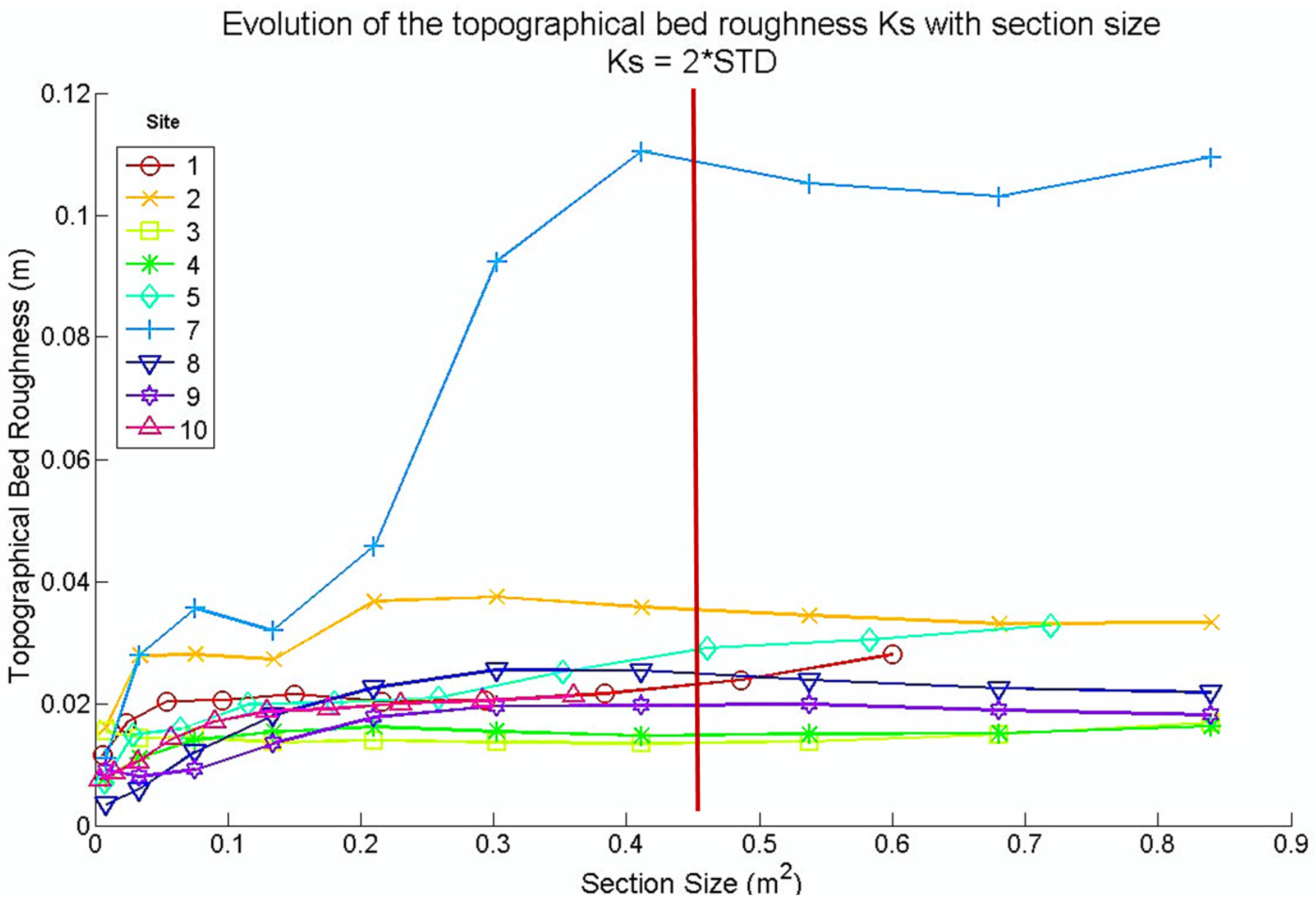
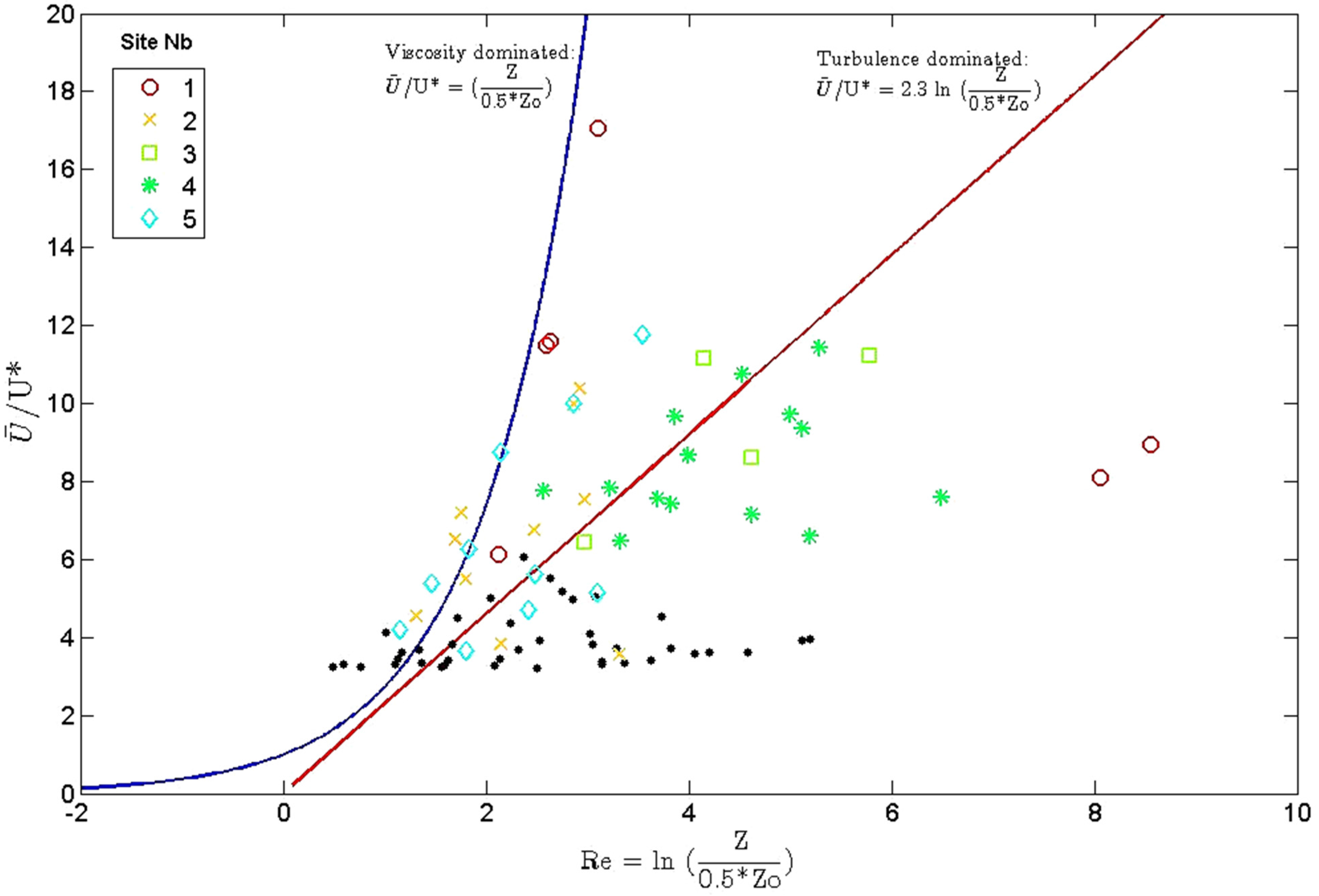
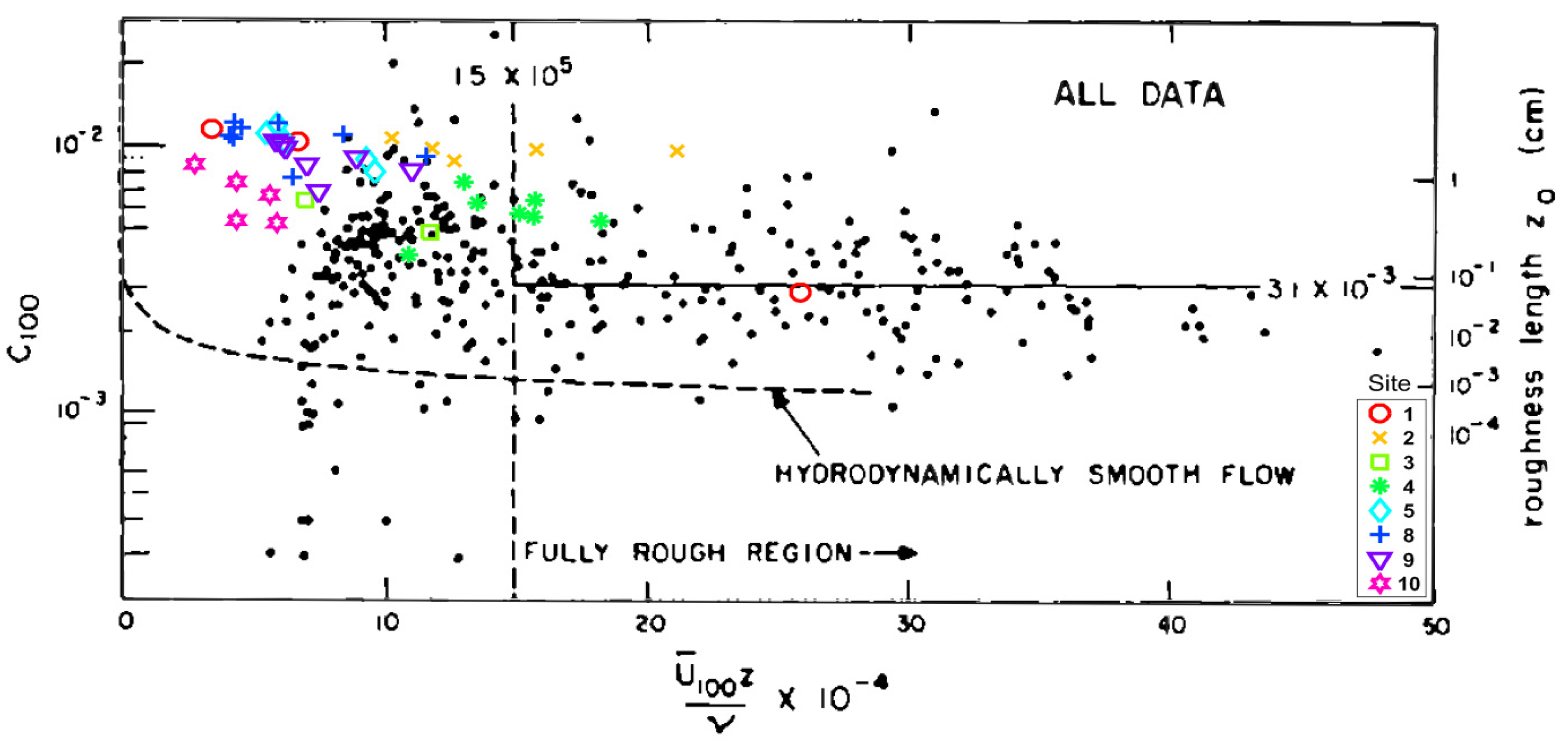
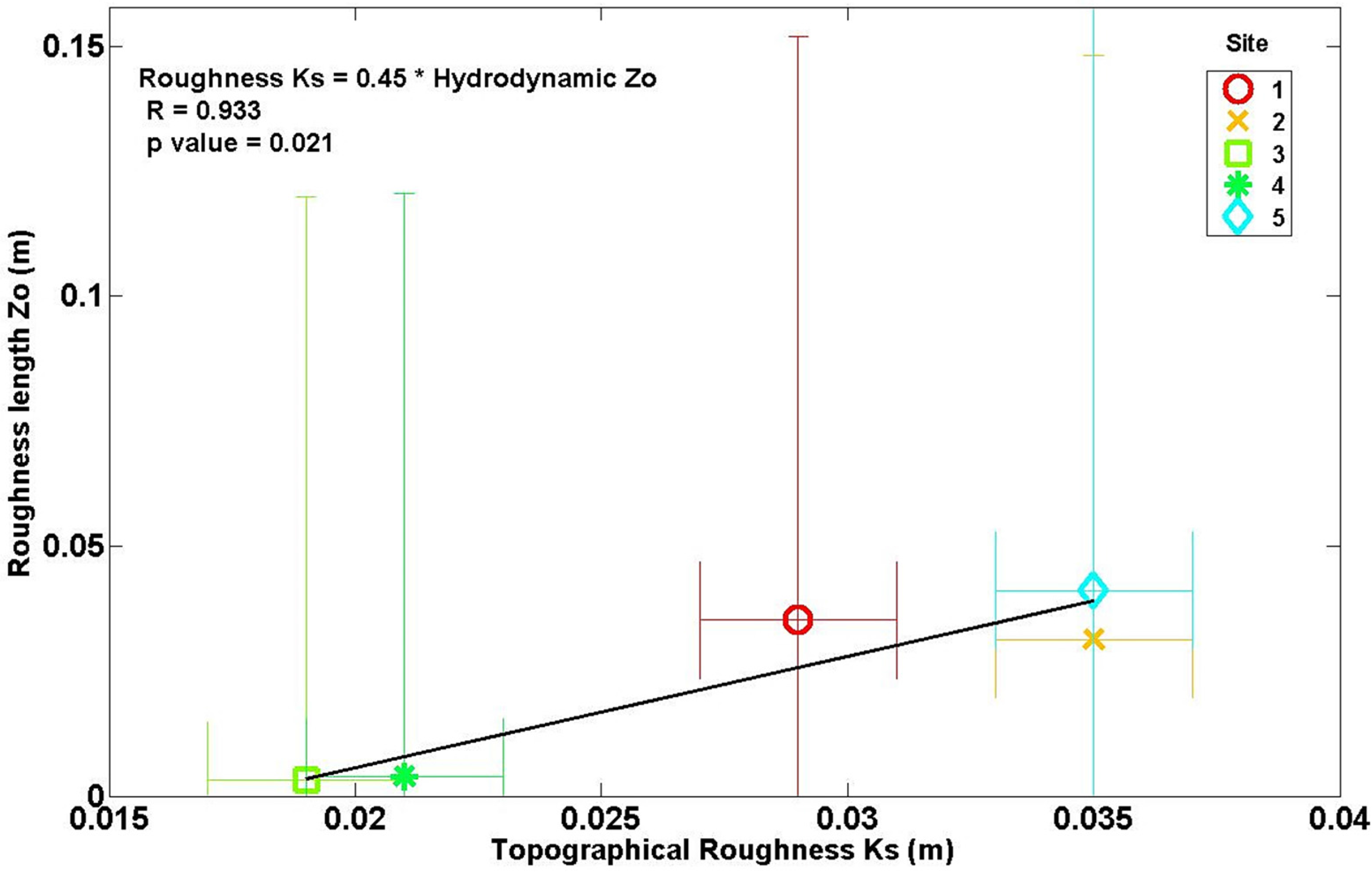
3.2. Relationship between Ks and Zo

3.3. Interpretations and Limits

3.4. Future Development
4. Conclusions
Acknowledgments
Author Contributions
Conflicts of Interest
References
- Komar, P.D. Boundary layer flow under steady unidirectional currents. In Marine Sediment Transport and Environmental Management; Jonh Wiley & Sons: New York, NY, USA, 1976; pp. 91–106. [Google Scholar]
- Dyer, K.R. Coastal and Estuarine Sediment Dynamics; Wiley: Chichester, UK, 1986; pp. 1–195. [Google Scholar]
- Villacieros-Robineau, N.; Herrera, J.L.; Castro, C.G.; Piedracoba, S.; Roson, G. Hydrodynamic characterization of the bottom boundary layer in a coastal upwelling system (Ria de Vigo, NW Spain). Cont. Shelf Res. 2013, 68, 67–79. [Google Scholar] [CrossRef]
- Clauser, F.H. The turbulent boundary layer. Adv. Appl. Mech. 1956, 4, 1–51. [Google Scholar]
- Heathershaw, A. The turbulent structure of the bottom boundary layer in a tidal current. Geophys. J. Int. 1979, 58, 395–430. [Google Scholar] [CrossRef]
- Thompson, C.E.L.; Amos, C.L.; Angelaki, M.; Jones, T.E.R.; Binks, C.E. An evaluation of bed shear stress under turbid flows. J. Geophys. Res. 2006, 111, 1–8. [Google Scholar] [CrossRef]
- Best, J.L.; Leeder, M.R. Drag reduction in turbulent muddy seawater flows and some sedimentary consequences. Sedimentology 1993, 40, 1129–1137. [Google Scholar] [CrossRef]
- Amos, C.L.; Feeney, T.; Sutherland, T.F.; Luternauer, J.L. The stability of fine-grained sediments from the Fraser River Delta. Estuar. Coast. Shelf Sci. 1997, 45, 507–524. [Google Scholar] [CrossRef]
- Cloutier, D.; LeCouturier, M.N.; Amos, C.L.; Hill, P.R. The effects of suspended sediment concentration on turbulence in an annular flume. Aquat. Ecol. 2006, 40, 555–565. [Google Scholar] [CrossRef]
- Thompson, C.E.L. The Role of the Solid-transmitted Bed Shear Stress of Mobile Granular Material on Cohesive Bed Erosion by Unidirectional Flow. Ph.D. Thesis, University of Southampton, Southampton, UK, 2003; pp. 1–214. [Google Scholar]
- Lefevbre, A. Bed Roughness over Vegetated Beds: Sonar Imaging Techniques and Effect on Unidirectional Currents. Ph.D. Thesis, University of Southampton, Southampton, UK, 2009; pp. 1–232. [Google Scholar]
- Burchard, H.; Craig, P.D.; Gemmrich, J.R.; van Haren, H.; Mathieu, P.-P.; Meier, H.E.M.; Smith, W.A.M.N.; Prandke, H.; Rippeth, T.P.; Skyllingstad, E.D.; et al. Observational and numerical modeling methods for quantifying coastal ocean turbulence and mixing. Prog. Oceanogr. 2008, 76, 399–442. [Google Scholar] [CrossRef]
- Lefebvre, A.; Lyons, A.P.; Thompson, C.E.L.; Amos, C. A new system for seafloor characterisation: BRAD, the Benthic Roughness Acoustic Device. In Proceedings of the International Conference on Underwater Acoustic Measurements: Technology and Results, Southampton, UK, 21–26 June 2009; pp. 1–8.
- Nelson, T.R. Benthic Boundary Layer Processes: Bedform Evolution and Bottom Turbulence. Ph.D. Thesis, University of South Carolina, Columbia, SC, USA, 2013; pp. 1–244. [Google Scholar]
- Nikuradse, J. Strömungsgesetze in Rauhen Rohren; VDI-verlag: Düsseldorf, Germany, 1933. [Google Scholar]
- Liu, Z. Sediment Transport; Aalborg Universitet: Copenhagen, Denmark, 2001; pp. 54–56. [Google Scholar]
- Middleton, G.V.; Southard, J.B. Mechanics of sediment movement. In Society of Economic Paleontologists and Mineralogists; California University: Los Angeles, CA, USA, 1984; pp. 1–401. [Google Scholar]
- Soulsby, R.L. The bottom boundary layer of shelf seas. Elsevier Oceanogr. Ser. 1983, 35, 189–266. [Google Scholar]
- Chriss, T.M.; Caldwell, D.R. Universal similarity and the thickness of the viscous sublayer at the ocean floor. J. Geophys. Res. 1984, 89, 6403–6414. [Google Scholar] [CrossRef]
- Guerrero, M.; Lamberti, A. Flow field and morphology mapping using ADCP and multibeam techniques: Survey in the Po River. J. Hydraul. Eng. 2011, 137, 1576–1587. [Google Scholar] [CrossRef]
- Wheatcroft, R.A. Temporal variation in bed configuration and one-dimensional bottom roughness at the mid-shelf STRESS site. Cont. Shelf Res. 1994, 14, 1167–1190. [Google Scholar] [CrossRef]
- Nikora, V.I.; Goring, D.G.; Biggs, B.J.F. On gravel-bed roughness characterization. Water Resour. Res. 1998, 34, 517–527. [Google Scholar] [CrossRef]
- Aberle, J.; Nikora, V.; Henning, M.; Ettmer, B.; Hentschel, B. Statistical characterization of bed roughness due to bed forms: A field study in the Elbe River at Aken, Germany. Water Resour. Res. 2010, 46, 1–11. [Google Scholar] [CrossRef]
- Bertin, S.; Friedrich, H. Measurement of gravel-bed topography: Evaluation study applying statistical roughness analysis. Am. Soc. Civil Eng. 2014, 140, 269–279. [Google Scholar] [CrossRef]
- Ferrarin, C.; Umgiesser, G. Hydrodynamic modelling of a coastal lagoon: The Cabras lagoon in Sardinia, Italy. Ecol. Model. 2006, 188, 340–357. [Google Scholar] [CrossRef]
- De Falco, G.; Magni, P.; Teräsvuori, L.M.H.; Matteucci, G. Sediment grain size and organic carbon distribution in the Cabras lagoon (Sardinia, Western Mediterranean). Chem. Ecol. 2004, 20, 367–377. [Google Scholar] [CrossRef]
- Magni, P.; De Falco, G.; Como, S.; Casu, D.; Floris, A.; Petrov, A.N.; Castelli, A.; Perilli, A. Distribution and ecological relevance of fine sediments in organic-enriched lagoons: The case study of the Cabras lagoon (Sardinia, Italy). Mar. Pollut. Bull. 2008, 56, 549–564. [Google Scholar] [CrossRef] [PubMed]
- Simeone, S.; Cucco, A.; Como, S.; De Falco, G.; Magni, P.; Perilli, A. Sediment distribution and hydrodynamic patterns in the Cabras lagoon, Sardinia (Italy). In Proceedings of the 16th Meeting of the Italian Society of Ecology, Viterbo, Italy, 19–22 September 2006; pp. 1–6.
- Moore, S.A.; Le Coz, J.; Hurther, D.; Paquier, A. On the use of horizontal-ADCPs for sediment flux measurements in rivers. In Proceedings of the 34th World Congress of the International Association for Hydro-Environment Research and Engineering: 33rd Hydrology and Water Resources Symposium and 10th Conference on Hydraulics in Water Engineering; Engineers Australia: Barton, Australia, 2011; pp. 3659–3666. [Google Scholar]
- Goring, D.G.; Nikora, V.I. Despiking acoustic doppler velocimeter data. J. Hydraul. Eng. 2002, 128, 117–126. [Google Scholar] [CrossRef]
- Mori, N.; Suzuki, T.; Kakuno, S. Noise of acoustic doppler velocimeter data in bubbly flows. J. Eng. Mech. 2007, 133, 122–125. [Google Scholar] [CrossRef]
- Chanson, H.; Trevethan, M.; Koch, C. Discussion of “Turbulence Measurements with Acoustic Doppler Velocimeters” by Carlos M. García, Mariano I. Cantero, Yarko Niño, and Marcelo H. García. J. Hydraul. Eng. 2007, 133, 1283–1286. [Google Scholar] [CrossRef]
- Sternberg, R.W. Friction factors in tidal channels with differing bed roughness. Mar. Geol. 1967, 6, 243–260. [Google Scholar] [CrossRef]
- Stapleton, K.R.; Huntley, D.A. Seabed stress determinations using the inertial dissipation method and the turbulent kinetic energy method. Earth Surf. Process. Landf. 1995, 20, 807–815. [Google Scholar] [CrossRef]
- Schlichting, H.; Gersten, K.; Gersten, K. Boundary-Layer Theory; Springer: New York, NY, USA, 2000; pp. 1–799. [Google Scholar]
- Ghasemi, A.; Zahediasl, S. Normality tests for statistical analysis: A guide for non-statisticians. Int. J. Endocrinol. Metab. 2012, 10, 486–489. [Google Scholar] [CrossRef] [PubMed]
- Styles, R. Flow and turbulence over an oyster reef. J. Coast. Res. 2015, 31, 978–985. [Google Scholar] [CrossRef]
- Friedrichs, C.T.; Wright, L.D.; Hepworth, D.A.; Kim, S.C. Bottom-boundary-layer processes associated with fine sediment accumulation in coastal seas and bays. Cont. Shelf Res. 2000, 20, 807–841. [Google Scholar] [CrossRef]
- Molinaroli, E.; Guerzoni, S.; De Falco, G.; Sarretta, A.; Cucco, A.; Como, S.; Simeone, S.; Perilli, A.; Magni, P. Relationships between hydrodynamic parameters and grain size in two contrasting transitional environments: The Lagoons of Venice and Cabras, Italy. Sediment. Geol. 2009, 219, 196–207. [Google Scholar] [CrossRef]
- Manca, E.; Cáceres, I.; Alsina, J.M.; Stratigaki, V.; Townend, I.; Amos, C.L. Wave energy and wave-induced flow reduction by full-scale model Posidonia oceanica seagrass. Cont. Shelf Res. 2012, 50–51, 100–116. [Google Scholar]
- Friedrich, H.; Spiller, S.M.; Rüther, N. Near-bed flow over a fixed gravel bed. In River Flow; Taylor & Francis: London, UK, 2014; pp. 1–279. [Google Scholar]
- Maleika, W.; Palczynski, M.; Frejlichowski, D. Interpolation methods and the accuracy of bathymetric seabed models based on multibeam echosounder data. In Intelligent Information and Database Systems; Springer: Berlin, Germany, 2012; pp. 466–475. [Google Scholar]
© 2015 by the authors; licensee MDPI, Basel, Switzerland. This article is an open access article distributed under the terms and conditions of the Creative Commons Attribution license ( http://creativecommons.org/licenses/by/4.0/).
Share and Cite
Chirol, C.; Amos, C.L.; Kassem, H.; Lefebvre, A.; Umgiesser, G.; Cucco, A. The Influence of Bed Roughness on Turbulence: Cabras Lagoon, Sardinia, Italy. J. Mar. Sci. Eng. 2015, 3, 935-956. https://doi.org/10.3390/jmse3030935
Chirol C, Amos CL, Kassem H, Lefebvre A, Umgiesser G, Cucco A. The Influence of Bed Roughness on Turbulence: Cabras Lagoon, Sardinia, Italy. Journal of Marine Science and Engineering. 2015; 3(3):935-956. https://doi.org/10.3390/jmse3030935
Chicago/Turabian StyleChirol, Clémentine, Carl L. Amos, Hachem Kassem, Alice Lefebvre, Georg Umgiesser, and Andrea Cucco. 2015. "The Influence of Bed Roughness on Turbulence: Cabras Lagoon, Sardinia, Italy" Journal of Marine Science and Engineering 3, no. 3: 935-956. https://doi.org/10.3390/jmse3030935
APA StyleChirol, C., Amos, C. L., Kassem, H., Lefebvre, A., Umgiesser, G., & Cucco, A. (2015). The Influence of Bed Roughness on Turbulence: Cabras Lagoon, Sardinia, Italy. Journal of Marine Science and Engineering, 3(3), 935-956. https://doi.org/10.3390/jmse3030935