1. Introduction
The LaHave River is an estuarine river in southern Nova Scotia that has a history of both fluvial and coastal flooding. Heavy rain and snowmelt can cause the river to overflow its banks, flooding the rural communities and roads within the watershed, while storm surge and sea-level rise can cause flooding near the coast; when a heavy rainfall event is combined with a storm surge, infrastructure within the watershed is especially at risk.
This project builds on a previous study which focused on the town of Bridgewater, Nova Scotia, which is located within the LaHave River watershed [
1]. In this study we expand the domain to model the entire watershed, and present modifications to the modelling in order to best represent the large and complex system. Here, as in the Bridgewater study [
1] we use a seamless digital elevation model (DEM) generated using high resolution lidar elevation data, bathymetric river data, and river cross-section information, along with river discharge and tidal elevation data to run a hydrodynamic model to produce flood risk predictions. The expanded study area necessitated augmenting our previous methodology of integrating the high resolution topography data with the various sources of bathymetric data. Like Merwade and Cook [
2], we approached the generation of the continuous topographic-bathymetric surface using GIS techniques.
Instead of the nested-grid approaches used in the past, in this study we employ a two-dimensional flexible mesh model, a more sophisticated and more appropriate model for the complex LaHave watershed. We use the DHI Mike Flexible Mesh model which represents a two-dimensional model of the river channel and floodplain. Flexible meshes, also known as unstructured triangular grids, are composed of triangles that can be varied in size throughout the mesh allowing the user to refine the mesh density to be higher in more critical areas and lower in less sensitive regions. This has the advantage of having higher resolution results where required while reducing computational costs in areas where only a coarse resolution is required, such as in deeper bathymetries. Additionally, flexible meshes adapt easily to follow the often irregular features of coastal and riverine systems better than rectilinear grids.
Flexible mesh modeling is a widely used and desirable basis for coastal flood models [
3,
4,
5] as well as river models [
6,
7,
8]. Shubert
et al. [
3] use an unstructured mesh to model coastal flooding in Glasgow, Scotland using lidar terrain data; they note the benefits of the flexible mesh density in urban areas. Kliem
et al. [
4] simulated storm surge for the North Sea-Baltic Sea using the varying resolution irregular mesh 2D shallow water model MOG2D to overcome the limitations imposed by regular grids for flood modelling. Wang
et al. [
5] used the unstructured triangular finite volume model FVCOM to more accurately represent shorelines and bathymetry; the authors coupled the hydrodynamic model with a GIS to visualize and analyze the results and found that the simulations agreed well with observations. Hagen [
6] and Gama
et al. [
7] used the Deltares-Flow-Flexible Mesh model to predict flood extent and both cited improvements in their ability to represent complex river geometries over structured grids.
Another improvement over Webster
et al. [
1] is the implementation of a spatially variable surface roughness map. Many have shown the importance of, and the differences between, including resistance parameters (e.g., Manning’s n or M) through satellite imagery [
8,
9], landcover classification data [
3], and lidar-based feature height data [
10,
11]. The collection of bathymetric data for rivers and shallow coastal areas is still a challenge, although new technology in the form of topo-bathymetric lidar provides the potential to acquire detail in shallow areas at a similar resolution and accuracy as traditional topographic lidar. Campana
et al. [
12] used bathymetric lidar to measure the topographic change of a river in the Italian Alps compared to manual river cross-section measurements. They conclude that bathymetric lidar offers great potential to monitor river evolution and to quantify morphological diversity. Kinzel
et al. [
13] compared the United States Geological Survey’s hybrid topographic/bathymetric Experimental Advanced Airborne Research LiDAR (EAARL) sensor with detailed surveys of river channels collected using wading and sonar techniques for rivers in California and Colorado. They showed that the lidar elevation of the river bed matched the traditional survey data to on average within 30 cm. They note that the water clarity must be sufficiently clear and that the albedo river bottom must be sufficiently reflective to produce laser returns to the sensor.
1.1. Study Area
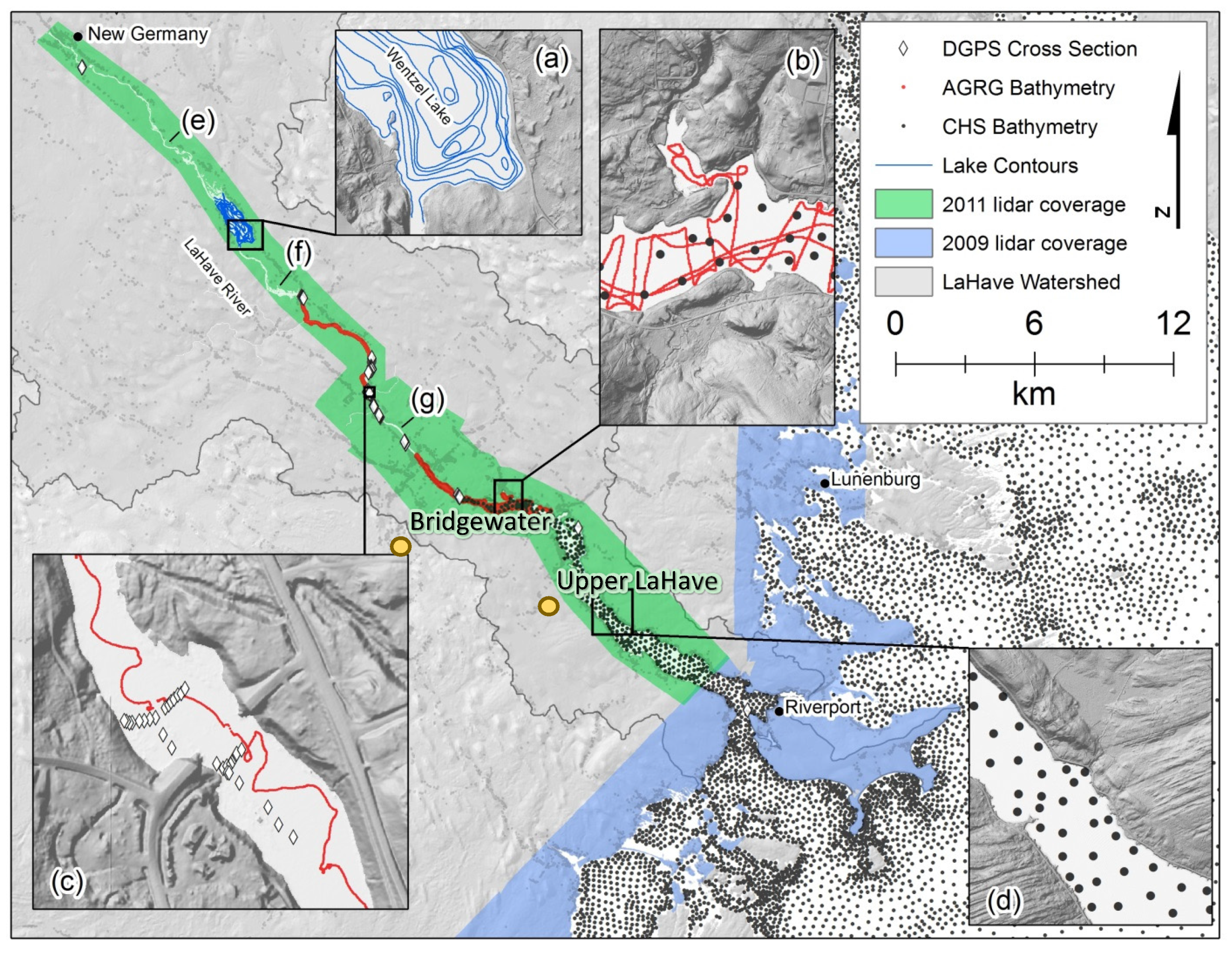
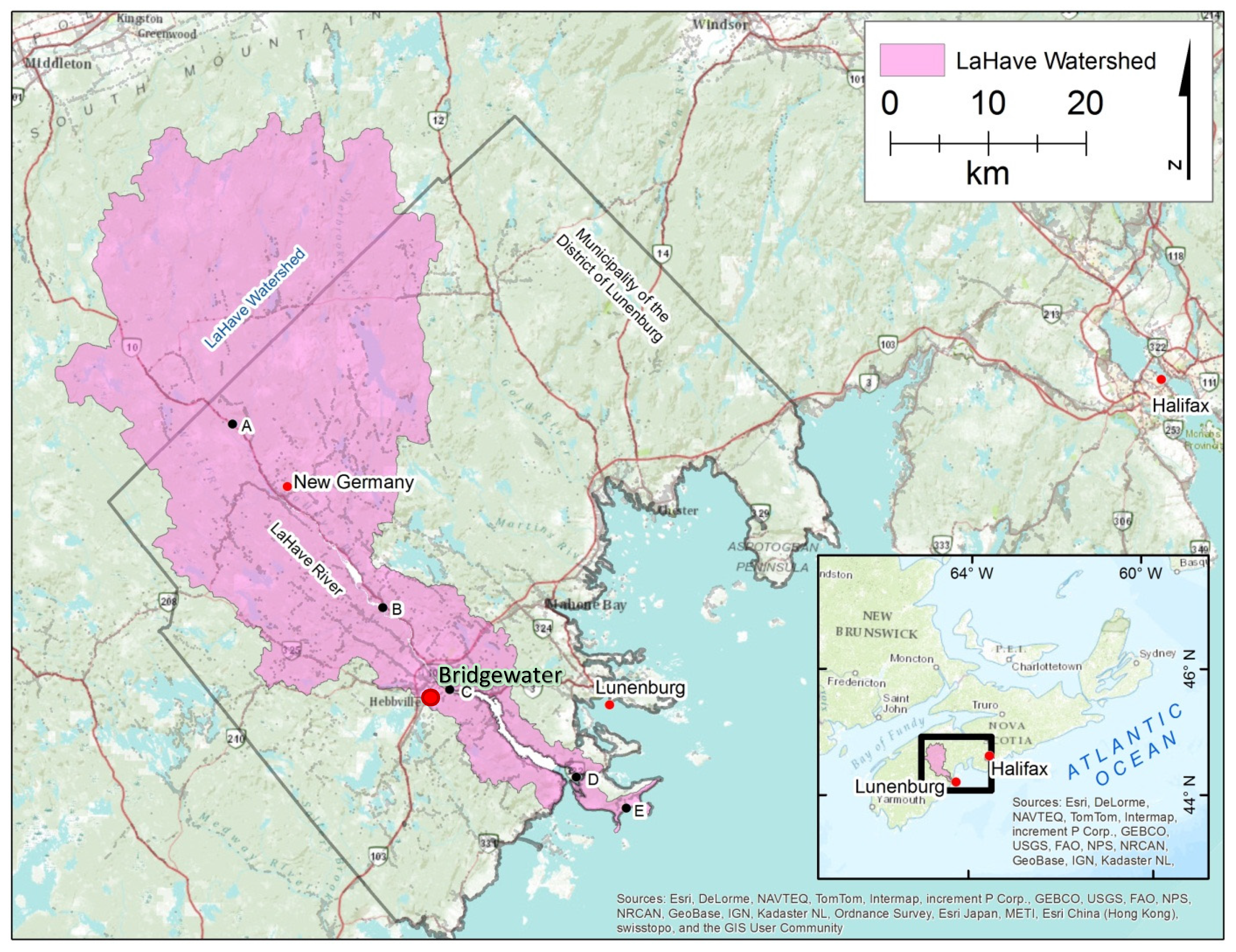
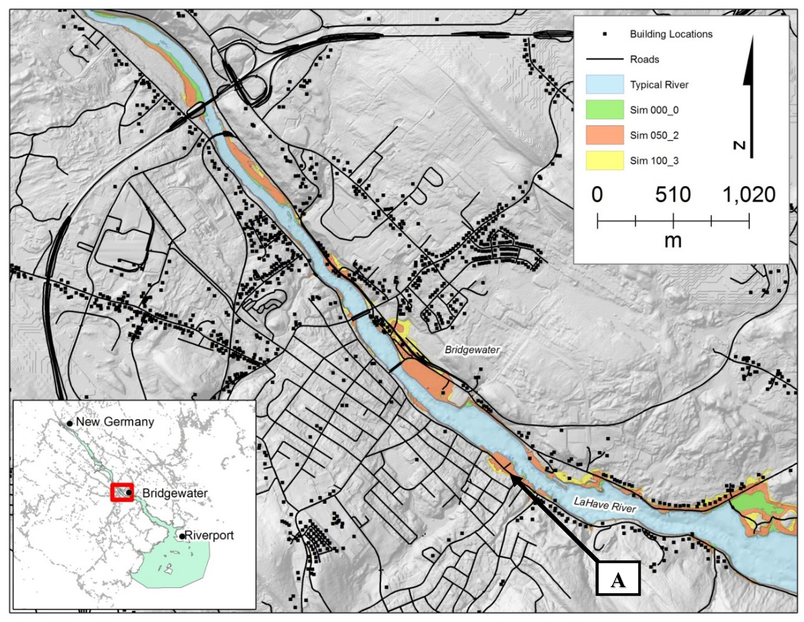
The LaHave River extends ~80 km from its headwaters at the southern base of South Mountain in the Annapolis Valley of Nova Scotia to its mouth on the Atlantic Ocean (
Figure 1). The river passes through several rural communities, reaches the Town of Bridgewater approximately 20 km from the Atlantic Ocean, and passes through several more small communities before meeting the coast. The LaHave River watershed drains many lakes and rivers, covers 1686 km
2, and encompasses sections of three counties and several municipalities, including the District of the Municipality of Lunenburg, for whom this study was completed. The watershed contains a mix of land use, including industrial and residential within the Town of Bridgewater, and shifting to mainly forested and agricultural in the majority of the watershed.
The LaHave watershed includes two Ecodistricts, as defined by the Nova Scotia Department of Natural Resources [
14]. The LaHave Drumlins Ecodistrict is characterized by glacial till drumlins and coniferous forests, with soils that are mostly well-drained, except between the drumlins where soil is poorly drained. The LaHave River flows through the center of the Ecodistrict until it enters the South Shore Ecodistrict near the coast. The South Shore Ecodistrict is composed of a mixture of sandy beaches, lakes and streams, and coastal forests.
Tides are semi-diurnal in the Bridgewater area, with a tidal range of 2.5 m. The tidal influence extends ~20 km up the LaHave River, just to downtown Bridgewater. The river does not ice over during the winter, but ice does form upstream of the town and in the lakes and throughout the watershed.
Figure 1.
The LaHave River watershed extends from South Mountain, Nova Scotia, to the Atlantic Coast. (A) Applied Geomatics Research Group (AGRG) Cherryfield weather station; (B) Environment Canada water level gauge; (C) AGRG Marine Terminal tide gauge at Bridgewater; (D) AGRG Kraut Point tide gauge; (E) AGRG Hirtles Beach weather station.
1.2. Flood History
Storm surges can occur along the Atlantic coast when low pressure systems such as hurricanes, post-tropical storms, and Nor’easters cause high winds and heavy rain. Typically the coastal zone bears the brunt of these types of storms, but a 1 m storm surge can cause flooding and road closures 20 km inland as far as downtown Bridgewater, as occurred on 30 October No storm surge return period analysis has been completed for the LaHave Estuary directly because there is no tidal record for the area; instead, the Halifax tide gauge, located 60 km northeast along the Atlantic Coast is used for analysis (
Figure 1).
Overland flooding of the LaHave River that results in property and infrastructure damage within the watershed occurs frequently and is caused by intense or prolonged rainfall, melting snow and ice, or a combination of these. Flow in the LaHave River follows a typical pattern, with maximum flow occurring in the spring and minimum flow occurring in the summer. An analysis of the 95-year LaHave River flow time series derived from the Environment Canada (EC) water level gauge in West Northfield (
Figure 1) shows that almost 80% of the floods during that time period occurred during winter or spring, times when snow melt is likely to have contributed to the flood [
15]. Maximum Instantaneous Peak Flow was highest on 10 January 1956 (1080 m
3/s) and second-highest on 31 March 2003 (663 m
3/s). Both of these floods were caused by heavy rain and melting snow and caused the highest water levels ever recorded (5.73 m and 5.17 m for 1956 and 2003, respectively), 1.5 to 2.0 m higher than any other flood event in the LaHave River watershed [
15]. Two fatalities occurred upstream of Bridgewater in 2003 when a car was swept off the road and into the flooded river [
16].
1.3. Climate Change
In the past ten years there have been 12 Storm Surge Warnings issued by EC for Lunenburg County [
17]; of these, only two events (October 2011 and February 2013 [
18]) resulted in a significant storm surge and flooding. Rainfall warnings are issued far more often: eight were issued in 2013, fourteen in 2014 and six within the first three months of 2015 [
17]; several of these resulted in flooding with road closures, one of which was particularly dangerous [
19]. Webster
et al. [
1] showed that combined storm surge and rainfall events can produce water levels higher than would be seen with a single event, and that risk to Bridgewater is increased as sea level rises.
Much attention has been devoted on a global scale to predicting sea-level rise [
20,
21,
22,
23]. The latest assessment of the Intergovernmental Panel on Climate Change (IPCC), AR5, projects a sea-level rise for 2046–2065 of 0.17 m to 0.38 m and for 2081–2100 of 0.26 m to 0.82 m, including the effects of melting ice sheets [
22]. Rahmstorf
et al. [
24] have suggested a rise between 0.5 and 1.4 m from 1990 to In Maritime Canada many coastal areas have been deemed highly susceptible to sea-level rise [
25]. In Nova Scotia, global sea-level rise is compounded by crustal subsistence [
26] which contributes an estimated 0.16 m per century to relative sea-level rise [
27]. A comprehensive, community-by-community report prepared by Richards and Daigle [
28] provides estimated extreme total sea levels for Lunenburg, a neighboring community along the South Shore of Nova Scotia located northeast of the mouth of the LaHave estuary, using Rahmstorf
et al. [
24] as a basis for sea-level rise projections. Their report presents results for 10, 25, 50 and 100-year return periods, for years 2000, 2025, 2055, 2085 and 2100, and shows that a 10-year storm could result in a sea-level of 3.29 m by 2025, 0.86 m higher than HHWLT (Higher High Water Large Tide), and a 100-year storm in 2055 would increase water level to 3.80 m.
As is the case with temperature and sea-level, precipitation and river discharge patterns are changing with climate change. In Atlantic Canada there is evidence that heavy rainfall events are increasing in frequency [
29,
30] an observation that agrees with models and predictions [
28,
29,
31,
32]; the increase in rainfall is expected to occur in the winter and spring [
28,
31]. Increased and intensified rainfall is also observed and predicted for New England [
33,
34,
35]. Studies of streamflow patterns during the last 50 years show that maritime rivers in the Atlantic provinces have been experiencing lower summer flows, but higher flows in early winter and spring [
36,
37]. Streamflow is expected to increase with temperature and precipitation in the Atlantic region [
38], and spring flooding could become more common due to changes in late-winter early-spring precipitation patterns [
39].
2. Experimental Section
This project shares data and some data analysis and modelling techniques with a previous study in the same area [
1]. The cases of overlap in
Section 2 are identified and discussed briefly and the reader is referred to Webster
et al. [
1], while new developments are discussed in detail. The former category includes hydrological data collection and model simulation design, while the latter category includes the GIS techniques employed to integrate topographic lidar data with coarser bathymetric data and the use of an image-derived surface roughness map. Additionally, we employ a different model, so
Section 2.5 discusses the details of the flexible mesh generation, the model calibration, and boundary condition implementation.
2.1. Hydrology Data
The modelled factors driving the potential for flood risk in the LaHave Estuary include weather, river stage and tides; these data are required to run the hydrodynamic model and predict flood risk and were obtained and used in the previous Bridgewater study [
1]. Discharge data for the river runoff model are from the Environment Canada flow sensor [
15] (
Figure 1B), additional water level data were observed near Bridgewater (
Figure 1C) and near the mouth of the river (
Figure 1D) using AGRG pressure sensors. Air pressure data used to compensate the water level sensors came from AGRG weather stations in the center of the watershed (
Figure 1A) and the Atlantic coast (
Figure 1E).
2.2. DEM Development
An accurate representation of bathymetry and topography is essential for successful hydrodynamic flood risk modelling. In this study bathymetry data from a suite of data sources were combined with topographic lidar data to generate a continuous DEM that was used in the model.
2.2.1. Bathymetric Survey
A bathymetric grid was compiled from a variety of sources to accurately represent seabed, lakebed and river channel bathymetry as well as their geometries (
Figure 2). Lake bathymetry was obtained from the Nova Scotia Department of Fisheries and Aquaculture [
40] (
Figure 2a). Upstream of Bridgewater a combination of depths were measured using a depth sounder mounted on a canoe (
Figure 2b) and for extremely shallow locations RTK GPS and depth measurements were obtained manually by walking across the river (
Figure 2c), and from Bridgewater to Upper LaHave the depth sounder was mounted on a 15 foot aluminum boat. The Canadian Hydrographic Survey (CHS) nautical chart Chart 4381 at a scale of 1:38,900 was digitized to obtain soundings between Upper LaHave and Riverport (
Figure 2d) and the digital chart covered the area from Riverport to the coast, including the mouth of the LaHave River. Areas where no bathymetric information existed were modelled to artificially form a channel using a method discussed in
Section 2.2.3 (
Figure 2e–g).
2.2.2. Lidar Survey
Lidar data for this project were obtained for the coastal region in 2009 [
41] and for the remainder of the watershed in 2012 [
1] at ~1 m spacing. Two surface models were constructed from these data; a Digital Surface Model (DSM) which incorporates all the points and a bare-earth DEM which incorporates only the classified ground points.
Figure 2.
Topo-bathymetric data sets amalgamated in this study include (a) lake bathymetry contours; (b) AGRG bathymetry from canoe survey; (c) AGRG RTK GPS cross sections; (d) CHS bathymetry from paper chart; (e–g) areas of no bathymetric information where the channel was modified. Blue area represents the lidar coverage from 2009, green area represents the lidar coverage from 2012.
2.2.3. Topographic-Bathymetric Data Integration
The lidar survey provides sufficient detail to model the floodplain but it does not penetrate the water surface and must be combined with the bathymetry data to generate a seamless topo-bathymetric DEM that represents the topography above and below the water line. The water surface extent was delineated from the combined 2011 and 2009 lidar datasets on a 2 m spatial resolution using a custom built ArcGIS tool that is based on user input cross-sections, as described in Webster
et al. [
1]. The water surface was refined with additional cross-sections and manual digitization where necessary.
The process of integrating the bathymetry data with the lidar data differs from and improves upon the previous study [
1]. Here, all bathymetric data from New Germany to Riverport (
Figure 2) were averaged by depth into a 12 m grid; the digital CHS chart covering the coastal area was dealt with separately and is discussed later. The river bank was identified using the water surface extent and a 4 m landward buffer. Bathymetry points that were within a specified distance to the river bank were removed to reduce severe oscillations in subsequent bank-bathymetry interpolations. The river bank then contained only lidar points at 2 m resolution, and these were assigned a value of 0 m depth. The bank points were then integrated with the now 12 m gridded bathymetry points at 16 m resolution using a spline interpolation method, and resampled to a 4 m resolution water depth grid (“observed spline”). A buffer extending from the river bank points to 10 m landward of the lidar bank points was used in the spline to eliminate interpolation calculations occurring between river segments.
Where bathymetry data were nonexistent (
Figure 2e–g) an experimentally determined depth model was developed based on Euclidian distance from the banks in areas of known bathymetry, such that:
where
h is water depth relative to the bottom and
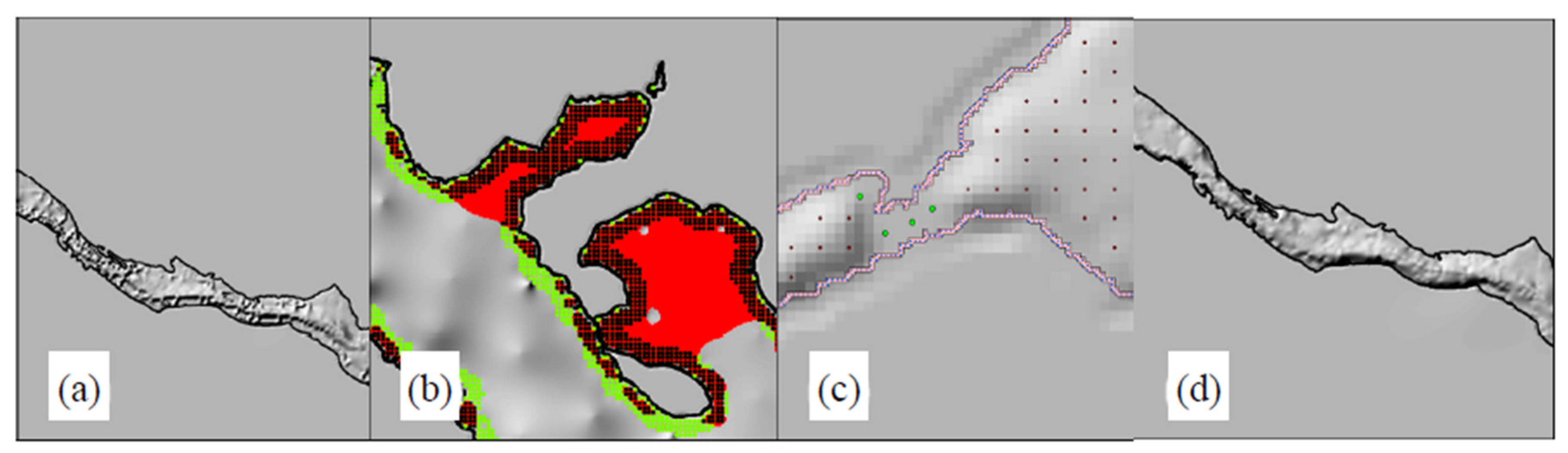
x is the Euclidian distance. Modelled depths were sampled to 12 m spacing and points within a 4 m distance of the river bank were removed. A spline was generated at a 4 m resolution using modelled and observed bathymetry points, lidar bank points, and a 10 m landward bank-buffered spline barrier (“modelled spline”). The resulting grid indicated that modelled depth values tended to over-estimate channel depth in some areas, specifically near the town of Bridgewater, producing an artificial scouring effect (
Figure 3a). This is to be expected as the depth model was designed to predict bathymetry further upstream where channel banks are steeper and the river is shallower. To combine the modelled and observed bathymetry more smoothly, a 1 bit raster mask was used to remove modelled bathymetry points in areas where the “modelled spline” depth points were more than 0.50 m deeper than the “observed spline” depth points (
Figure 3b). Furthermore, a manual estimation of water depth was included as points where some narrow sections of the LaHave water surface were unaccounted for by this technique (
Figure 3c) and the spline interpolation was recomputed to generate a final river bathymetry grid (
Figure 3d).
Figure 3.
(a) The initial modelled-observed bathymetry interpolation; (b) the mask used to remove poorly modelled bathymetric points: red points were kept and green points discarded; (c) the resultant spline with no artificial scouring; (d) additional bathymetry was added manually as required (green points).
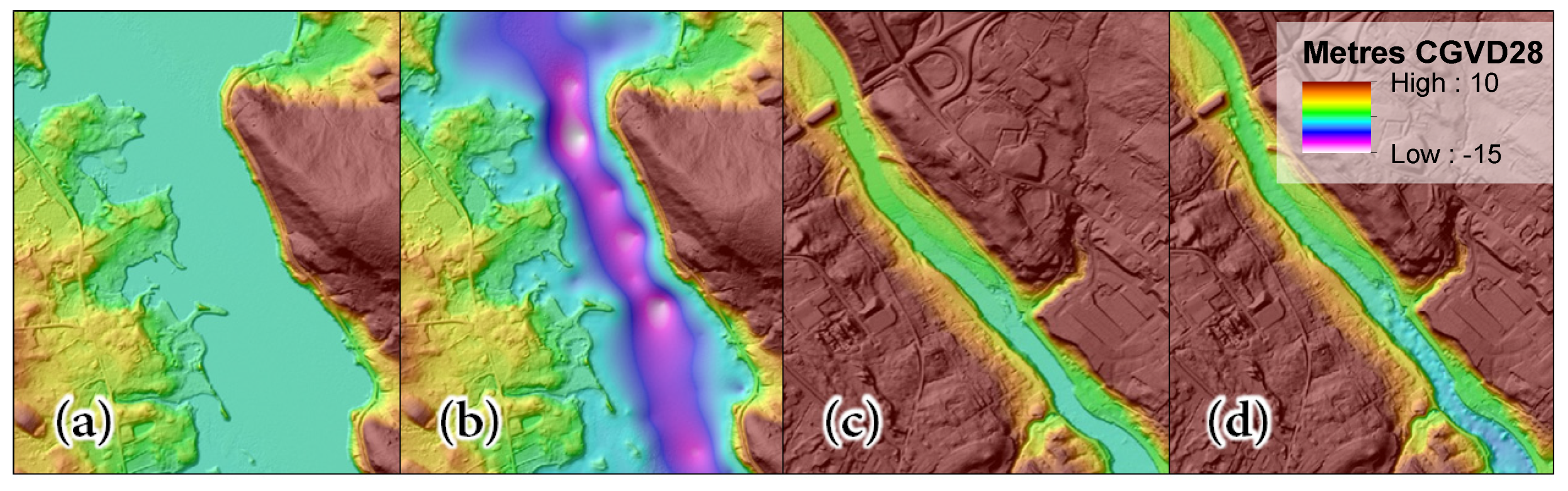
The river bathymetry grid was bi-linearly resampled to a 2 m spatial resolution and subtracted from the 2 m resolution lidar DEM with the water surface included (
Figure 4); this generated a DEM of lidar topography and river bathymetry for the lidar extent. Sections where noise, offsets, or artifacts existed in the water surface of the lidar were selected and smoothed using a low-pass filter, or removed. The tidal portion of the study area extended ~15 km from Riverport into the Atlantic Ocean (
Figure 2). This area was outside of the lidar extent and so was modelled using 20 m Nova Scotia Topographic Database (NSTDB) elevation data up to 10 m relative to the Canadian Geodetic Vertical Datum of 1928 (CGVD28) merged with the CHS digitized chart bathymetry; the resulting coastal DEM was merged with the river DEM to generate a seamless topographic-bathymetric model of the LaHave River estuary relative to CGVD28.
Figure 4.
Lidar data before (a,c) and after (b,d) bathymetric integration; An area upstream of Bridgewater is shown in (a,b); downtown Bridgewater is shown in (c,d).
Figure 4.
Lidar data before (a,c) and after (b,d) bathymetric integration; An area upstream of Bridgewater is shown in (a,b); downtown Bridgewater is shown in (c,d).
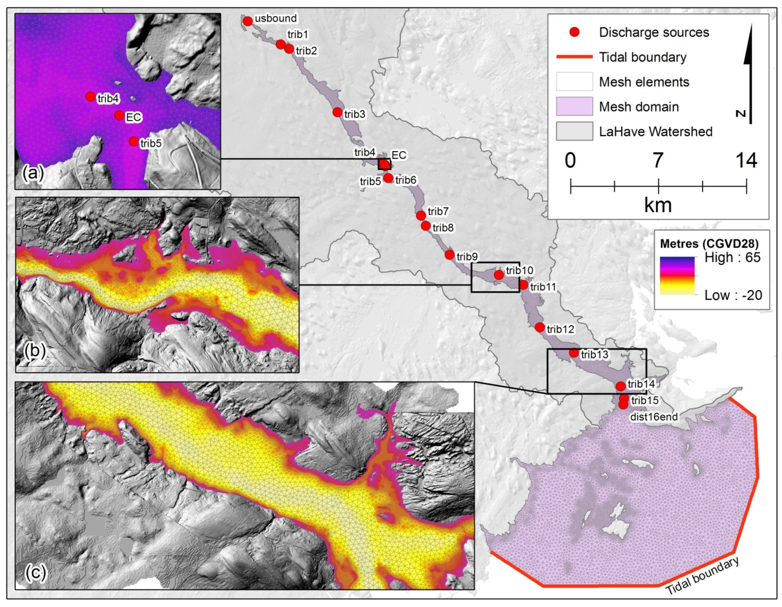
2.3. Unstructured Mesh Generation
An unstructured grid, or flexible mesh, was generated from the seamless 2 m topographic-bathymetric DEM using the Mike DHI mesh generator toolset (
Figure 5). Before computation of the flexible mesh, the modelled domain was limited to areas where flooding was possible by calculating a maximum flood extent. To accomplish this, the slope of the LaHave River level was determined through the use of a flow accumulation calculation, and an approximate maximum flood level (
zmax relative to CGVD28) along the river channel was calculated such that:
where
z refers to vertical elevation relative to CGVDThis function was developed such that the maximum flood level would be limited to 10 m above areas with a river level of 0 m CGVD28 (which can accommodate a storm surge of approximately 8.5 m if necessary) and flood levels upstream at the head of the river (62 m CGVD28) would have a maximum flood level of ~65 m CGVD28, or a maximum flood depth of ~3 m. The maximum flood extent was generated by buffering points along the river by a factor based on the flow accumulation, calculating the maximum flood level using Equation (2), and intersecting the resultant surface with the seamless DEM. The maximum flood extent was used to generate the outer boundary of the flexible triangular mesh grid (
Figure 5). The boundary was smoothed using the Polynomial Approximation with Exponential Kernel (PAEK) algorithm with a smoothing tolerance of 20 m to eliminate sharp angles of the boundary originating from the vectorization of the maximum water level raster.
The boundary was also used to clip the lidar elevation grid to reduce the input of elevation data into the Mike DHI mesh building tool. Topographic data density was reduced further using a key-point analysis to eliminate redundant elevations while preserving geometry to within 0.10 m; this technique reduces the number of points in a mesh but still provides an accurate representation of the topography. The mesh density was further customized to increase model stability and reduce simulation time by separating it into sections of varying mesh density. Mesh density near the river banks was defined to increase linearly with slope and elevation, and the remainder of the mesh was designed following the advancing-front method [
42] so that it varied in density from 50,000 m
2 maximum area per triangle element in the coastal region (
Figure 5c); to 500 m
2 in the densest regions upstream (
Figure 5a,b). All triangles were built with a minimum allowable angle of 26 degrees.
Figure 5.
Flexible mesh modelling domain with tidal and discharge (tributary) boundary locations. (a) Inset of the mesh at the EC gauge; (b) variable mesh density and elevation midway along the estuary; (c) variable mesh density and elevation midway near the mouth of the estuary.
Figure 5.
Flexible mesh modelling domain with tidal and discharge (tributary) boundary locations. (a) Inset of the mesh at the EC gauge; (b) variable mesh density and elevation midway along the estuary; (c) variable mesh density and elevation midway near the mouth of the estuary.
2.4. Surface Roughness Map
The stability and calibration of coupled coastal-fluvial hydrodynamic flood models depends in large part on the accurate representation of dynamic flow characteristics over varying surfaces such as cobbled streams, vegetation and concrete. As such, bed roughness indices were employed to model the observed relationship between depth-averaged flow velocity and total water depth across varying bed types. To represent this relationship spatially the model included a variable Manning’s M index grid, for which small numbers represent the roughest surfaces and most resistance to flow, and the largest numbers represent the smoothest surfaces and least resistance to flow; Manning’s M is the reciprocal of the commonly used Manning’s n. Here, we used a single Band 5 (near infrared) 30 m resolution Landsat 5 image (taken 27 July 2008) to develop a 10 m resolution surface roughness grid based on vegetation density and land use (
Table 1).
Table 1.
Derivation of Manning’s M spatial roughness grid.
Table 1.
Derivation of Manning’s M spatial roughness grid.
| Feature | Manning’s M |
|---|
| Vegetation | Heavy | Digital Number | 16–54 | 10 |
| Medium | 55–69 | 15 |
| Light–none | >70 | 20 |
| Initial value for river channel and coast | 25 |
| Roads | 90 |
2.5. Hydrodynamic Modelling
There are many approaches to the hydrodynamic modelling of estuarine systems, all with various levels of detail and requirements. This model was designed using the Mike DHI software wherein a 2-d depth averaged incompressible Reynolds averaged Navier-Stokes shallow-water equation was solved over the constructed flexible mesh domain with a variable time step scheme. Operationally the simulations ran at an average time step of approximately 0.4 s. The shallow water equations used allowed for variation in temperature, salinity, and density, but all were assumed constant in this study to decrease processing time. Ideally, discharge data would be available for each tributary entering the LaHave River to incorporate river discharge from the whole watershed into the downstream tidal model (
Figure 5). In the absence of these data, our approach was to include discharge from all major tributaries as discharge point sources, each scaled relative to a single long term observed discharge record which exists in the mid-section of the model domain. Catchments for the 17 tributaries were defined using a flow accumulation calculation for the entire LaHave watershed executed on a 20 m spatial resolution DEM using available NSTDB data. Each source point was assigned a scale factor based on the area of its catchment relative to the drainage area of the LaHave River EC gauge (
Table 2). Additional discharge sources intermediate to defined tributaries were included in tributary point sources downstream. The scale factors were applied to the EC daily discharge record [
15] resulting in a discharge time series for each tributary. This approach allowed the model to be linked to a large amount of discharge data for statistical purposes while not being required to analyze rainfall rates or the complexities of snow melt, both of which are inherent to the discharge record; additionally, we were able to incorporate contributions from all catchments without deploying sensors at each tributary location. This method is limited by the assumption that all catchments in the watershed have the same hydrological properties. The scaled discharge time series were used as boundary conditions that were varied for each model simulation and area discussed in
Section 2.5.2.
Table 2.
Major LaHave River tributaries, catchment contributions, and scale factor applied to the EC gauge discharge.
Table 2.
Major LaHave River tributaries, catchment contributions, and scale factor applied to the EC gauge discharge.
| Name | Catchment Contribution (Number of 20 × 20 m Pixels) | EC Gauge Ratio |
|---|
| EC Gauge | 3,113,163 | 1.00000 |
| usbound | 1,781,664 | 0.57230 |
| trib3 | 1,148,538 | 0.38428 |
| trib6 | 459,567 | 0.14796 |
| dist16end | 14,972 | 0.00481 |
2.5.1. Model Calibration
The model was calibrated by comparing observed water levels at the EC gauge, near the town of Bridgewater, and at the mouth of the river (locations shown on
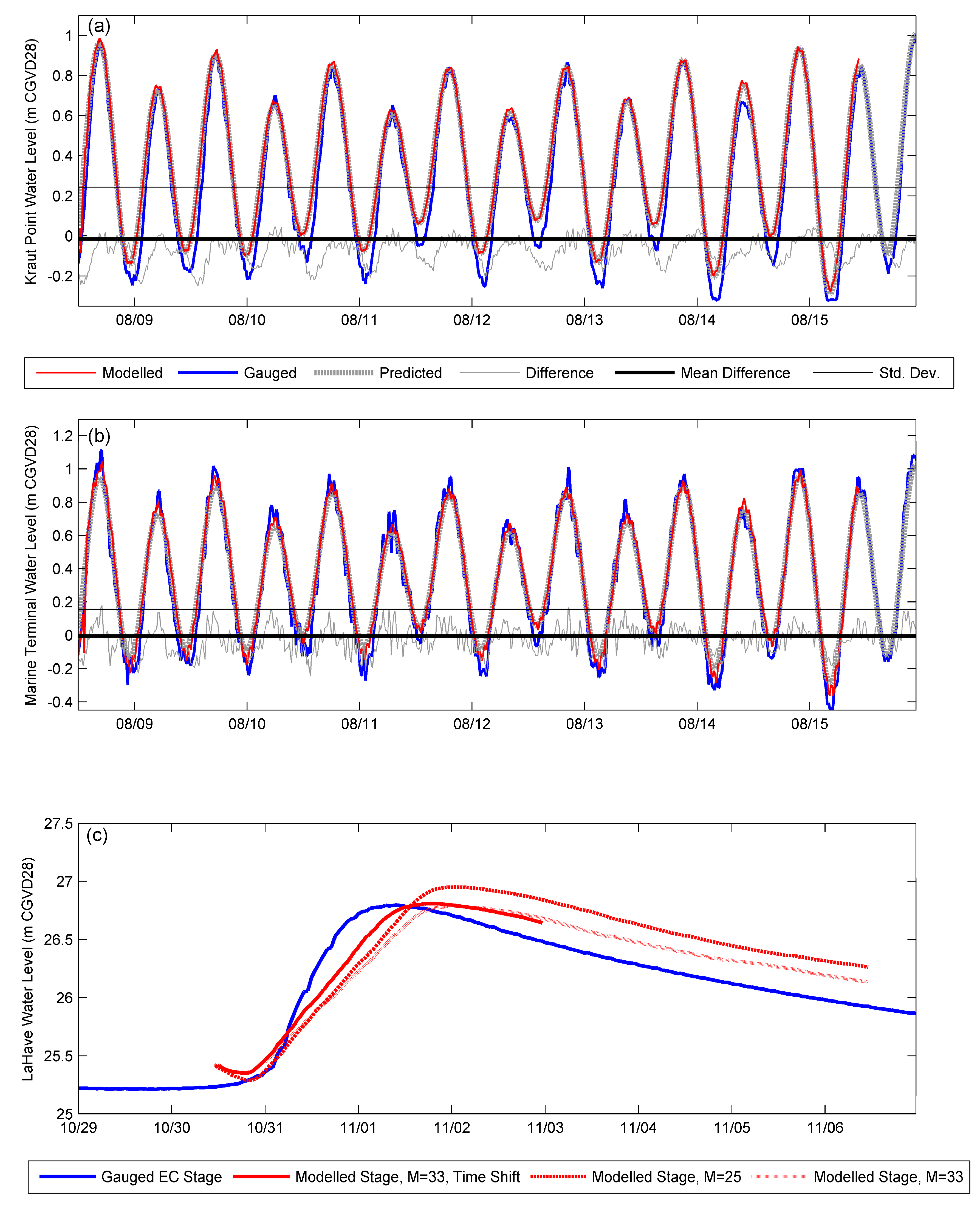
Figure 1) to modelled water levels extracted from the model at those locations. All water level recording equipment were referenced vertically to the datum of the model (CGVD28) using survey grade RTK GPS (with a precision of 2.5 cm or better). Tidal calibration was done for 8–15 August 2012 which was selected as a period where the predicted and gauged tides were most congruent and did not exhibit any high frequency variations observed during the winter (
Figure 6a,b). At Kraut Point (Marine Terminal) the mean difference between modelled and observed water level was −1.5 cm (−5.2 cm), standard deviation 24 cm (15 cm). This very low mean difference between the modelled and observed water levels in the southern portion of the model domain (Kraut Point,
Figure 1) indicates that the tidally dominated portion of the flow model operates very accurately, specifically during non-storm events. A discharge event on 1 November 2012 was used for the fluvial model calibration as the river water level conditions before the event were stable and the curve of the event was smooth and thus near the signature desired to be used for the various flood simulations (
Figure 6c).
In the calibration phase, all hydrodynamic parameters were determined and remained consistent for all subsequent flood scenario simulations (
Table 3). Principal parameters which contributed to the fluvial calibration include the relative timing of discharge sources upstream of the EC gauge as well as the bed roughness of the river. It was experimentally determined that each of the discharge sources upstream of the EC gauge (usbound, trib1, trib2, trib3) should be shifted by several hours (7, 5, 5, 2, respectively). A Manning M value of 33 was determined for the river channel and the coastal domain of the model using a trial and error process of model and observation time series comparison. A small section on the edge of the tidal boundary was assigned a very rough Manning M value of 5 to eliminate oscillations which existed along the boundary and thus improved model stability.
Table 3.
Final model parameter values.
Table 3.
Final model parameter values.
| Parameter | Value |
|---|
| Time step | Variable, 0.01–30 s |
| Critical CFL number | 0.8 |
| Drying Depth | 0 m |
| Flooding Depth | 0.05 m |
| Wetting Depth | 0.1 m |
| Density Type | Barotropic |
| Smagorinsky eddy viscosity coefficient | 0.28 |
| Final Manning M of river channel and most of coast | 33 |
| Final Manning M at tidal boundary | 5 |
Figure 6.
(a) Comparison of tide gauge observations with model results at Kraut Point (mean difference −1.5 cm, standard deviation 24 cm); (b) comparison of tide gauge observations with model results at the Marine Terminal (mean difference −5.2 cm, standard deviation 15 cm). Predicted tide used for the model boundary is plotted on both (a,b); (c) shows gauged and modelled stage of the LaHave River at the Environment Canada Gauge location. Three different model results are shown with variable Manning’s M; the final model version (solid red line) uses M = 33 and a time shift. Note that (a,b) share the same legend; (c) references the legend at the bottom of the figure.
2.5.2. Model Simulations
2.5.2.1. Extreme Value Analysis
In this study we are examining the risk of flooding from two possible sources which can interact to compound the problem: river runoff and storm surges or long-term sea-level rise. The model scenarios follow Webster
et al. [
1], who use extreme value models (EVMs) to determine the return periods of extreme events using the discharge and sea-level time series to examine how often such events have occurred in the past. The time series of measured discharge of the LaHave River (1915–2012) was used to determine the annual probability of extreme events and also the return period of extreme high flow events.
Table 4a summarizes the return period in years and the associated discharge for a 65% probability of occurrence, which equals at least one occurrence. Re-examining the historical high discharge events of January 1956 and March 2003, we see that the 1956 event has a recurrence interval greater than 100 years (1080 m
3/s), while the 2003 event (663 m
3/s) is approximately equivalent to a 50 year return period event with a 65% probability of occurrence.
Table 4.
Model simulations. Simulation naming scheme format: first 3 digits indicate a discharge return period of 0, 50 or 100 years, last digit indicates level of storm surge (0 for maximum high tide conditions, 2 for a 2.0 m surge on top of the predicted tide or 3 for a 3.0 m surge on top of the predicted tide).
| (a) LaHave River Scenario | (b) Sea Level Scenario |
|---|
| Probability | Return Period | Discharge (m3/s) | Max. High + 0.0 m | Max. High + 2.0 m | Max. High + 3.0 m |
|---|
| 65% | 0 year | 210 | Sim000_0 | Sim000_2 | Sim000_3 |
| 50 year | 652 | Sim050_0 | Sim050_2 | Sim050_3 |
| 100 year | 741 | Sim100_0 | Sim100_2 | Sim100_3 |
The Halifax tide gauge record (1920–2010) was used to estimate the risk or probability of flooding related to high water events along the coast [
1,
41]. The 100-year return period flood level under current RSL conditions is 2.2 m [
1], which is 10 cm below previous high water level maximum observed during Hurricane Juan in Halifax in 2003 which had an associated storm surge of 1.63 m [
27]. If RSL increases to a rate of 0.73 m/century [
21], the 100 year water level increases to 2.5 m CGVD28 which further inundates areas. If RSL increases to a rate of 1.46 m/century [
24], the 100 year water level increases to 3.1 m CGVDIn this study, we use these estimates as guidelines, and use storm surge levels of 0.0 m, 2.0 m and 3.0 m (
Table 4b) added to the maximum predicted high tide for These values can be thought of as extreme storm surges today or moderate surges in the future considering RSL.
Three sets of model simulations were executed for each different return period discharge: one set based on variable discharge under maximum high tide conditions in 2012, and two other sets based on different storm surge or long-term sea-level rise conditions (
Table 4).
2.5.2.2. Boundary Conditions
The discharge and storm surge scenarios were implemented using boundary conditions (
Figure 7). The river discharge boundary condition was scaled proportionally to the drainage area for the LaHave River as described above and varied according to the 0, 50 and 100 year return period discharge values (
Figure 7a,b). We obtained predicted water level time series from the DHI Global Tidal Model, which includes the 10 major tidal constituents [
43]. The storm surge scenarios (0.0 m, 2.0 m, and 3.0 m water levels) were added to the predicted maximum 2012 high tide boundary (
Figure 7c) at the mouth of the LaHave River (
Figure 5). The timing of the peak river discharge relative to the storm surge peak was determined experimentally, after calibrating for surface roughness, to ensure the worst case flooding condition.
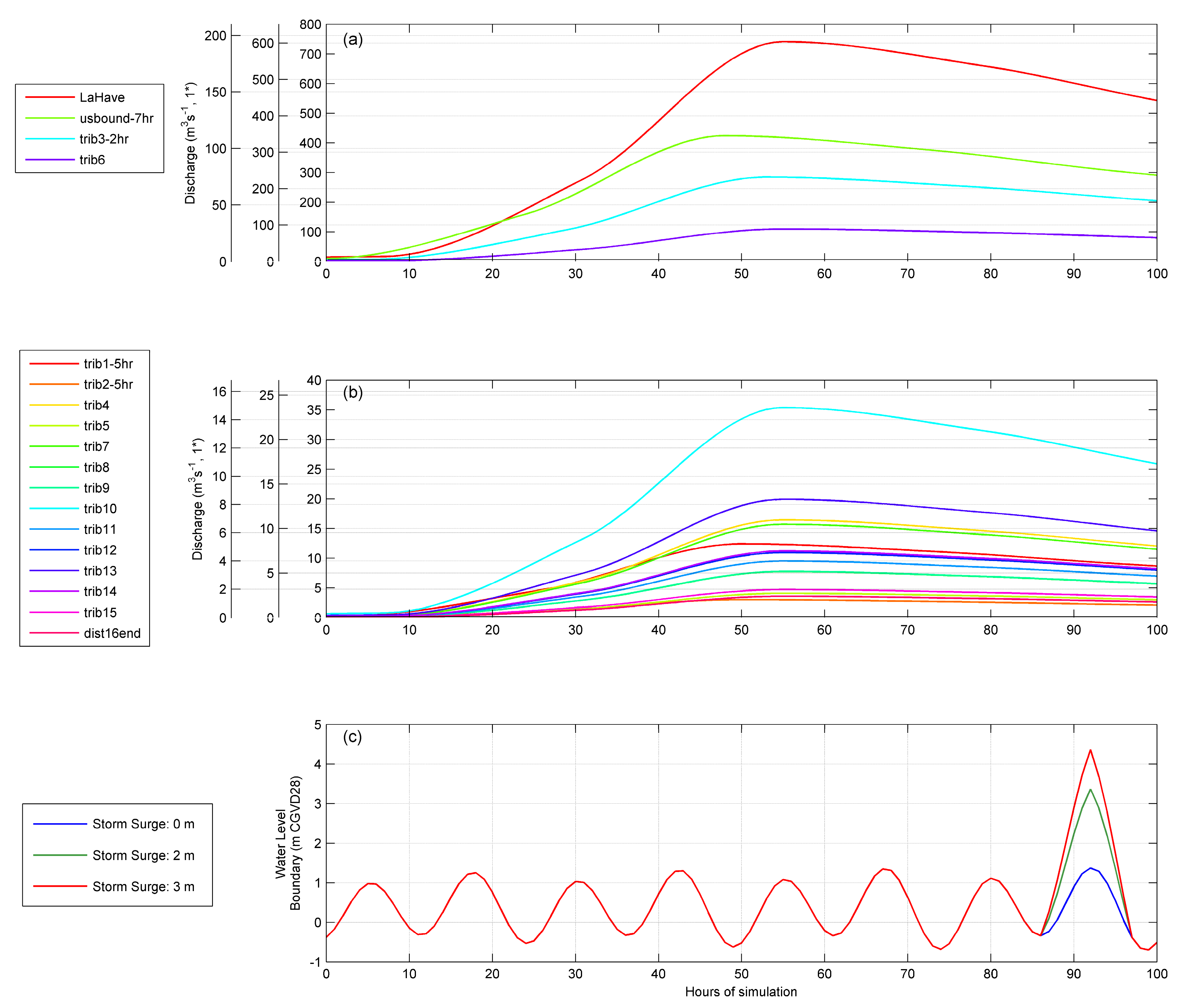
Figure 7.
Model Boundary Conditions for (a) discharge at major tributaries for 0, 50, and 100 year return level flows; (b) discharge at minor tributaries for 0, 50, and 100 year return level flows; (c) tidal boundaries for storm surge levels 0 m, 2 m, and 3 m.
Figure 7.
Model Boundary Conditions for (a) discharge at major tributaries for 0, 50, and 100 year return level flows; (b) discharge at minor tributaries for 0, 50, and 100 year return level flows; (c) tidal boundaries for storm surge levels 0 m, 2 m, and 3 m.
4. Conclusions
This study modelled combined river discharge and ocean tide-surge hydrodynamics to map flood risk using a combination of innovative GIS tools and methodologies and a sophisticated hydrodynamic model that was established for the study area using a flexible mesh representation of the hydrography and topography.
Discharge was simulated for events that represent a typical annual maximum runoff and extreme events with at least one occurrence within a 50 and 100 year return period based on the EC gauge time-series data measured upstream of Bridgewater. Tide and storm surge events or the equivalent of long term sea-level rise were simulated by using the predicted maximum high tide during 2012 and adding a 2 and 3 m storm surge to the ocean level seaward of the mouth of the river. In total nine simulations were carried out using a combination of three discharge levels coupled with three tidal-surge levels. For extreme events that are dynamic in nature, the maximum water level can occur at different places and at different times during the simulation. The maximum flood extent for each simulation was examined and the maximum water level for the duration of the simulation was extracted and merged into one file and used in the GIS to map the maximum flood extent and water depth.
Areas upstream of Bridgewater appear most vulnerable to fluvial discharge events and maps demonstrate the areas that are most vulnerable. Areas downstream of Bridgewater appear to be most vulnerable to storm surge and sea-level rise. Infrastructure including roads, buildings and the municipal wastewater (e.g., lift stations) were intersected with the flood layers to map areas at greatest risk. The road information was converted to points every 10 m and analyzed along with the building points and wastewater infrastructure where the flood depth information for each for each of the nine simulations was appended to their respective attribute tables. There are areas where the combined effects of large discharge with elevated sea-levels produce higher water levels than any single event on its own. No adaptation measures have been considered as that was beyond the scope of this current project. However, the information provided from this study will allow the municipality and provincial departments such as the Nova Scotia Department of Transportation and Infrastructure Renewal the ability to evaluate the risk of flooding from large river discharge events and storm surge or longer term sea-level rise and their combined effects and begin considering adaptation measures to mitigate flooding.


