Abstract
Polymetallic nodules are spherical or ellipsoidal mineral aggregates formed naturally in deep-sea environments. They contain a variety of metallic elements and are important solid mineral resources on the seabed. How best to quickly and accurately identify polymetallic nodules is one of the key questions of marine development and deep-sea-mineral-resource utilization. We propose a method that uses YOLOv5s as a reference network and integrates the IoU (Intersection over Union) and the Wasserstein distance in the optimal transmission theory to accurately identify different sizes of polymetallic nodules. Experiment using deep-sea hyperspectral data obtained from the Peru Basin was performed. The results showed that better recognition effects were achieved when the fusion ratio of overlap and Wasserstein distance metric was 0.5, and the accuracy of the proposed algorithm reached 84.5%, which was 6.2% higher than that of the original baseline network. In addition, the rest of the performance indexes were also improved significantly compared to traditional methods.
1. Introduction
Polymetallic nodules, also known as ferromanganese nodules, are mainly found in the surface layer of sediments on the seafloor of the world’s oceans [1]. They are formed at water depths of 3500–6500 m and are an important oceanic mineral resource [1,2]. Polymetallic nodules have a core consisting mainly of rock fragments, bone fragments or fragments of old nodules, and an outer shell layer composed mainly of Fe-Mn oxyhydroxides, which are formed around the core by hydrogenetic and diagenetic precipitation [3,4].
The morphology of polymetallic nodules is varied, with nodules being the most common and some also appearing as crusts or plates. The surface is black, brown, or tan [5]. The global polymetallic nodule prospecting area includes the Clarion-Clipperton fracture zone (CCZ) in the East Pacific Ocean, the Central Pacific Basin, and the Peru Basin, etc. [6]. In the 1890s, the study of polymetallic nodules began to attract attention globally [7], and in the 1960s, large-scale research and the study of oceanic polymetal resources began to be carried out globally [8]. With the increasing tensions regarding land resources, the development of oceanic solid mineral resources has become an important choice. The polymetallic nodules of the Peru Basin mainly contain Mn, Cu, and Ni, alongside trace amounts of other metal elements such as Co, The, Mo, Pt, and rare earth elements (REEs) [9,10,11,12,13]. These metallic elements are widely used in production in sophisticated industries and have a high economic value [14,15,16,17]. In recent years, deep-sea mining has gradually become an emerging and important industry, and seabed mineral resource investigation has been increasingly emphasized [10].
Traditional survey methods for polymetallic nodule resources include multi-beam acoustic detection, mechanical sampling, and optical image interpretation [18,19,20,21,22,23]. In recent years, the active hyperspectral image has been gradually applied to deep-sea resource surveying [24,25], which can carry out detailed surveying and characterization of seabed mineral deposits and allow understanding of the distribution of seabed resources [26,27,28]. Hyperspectral images contain hundreds or thousands of continuous narrow-band spectra [29]. A large amount of spectral data can provide more information and help with the investigation of deep-sea mineral resources. At present, the supervised learning method is widely used in the processing of underwater hyperspectral-image data. The supervised learning needs to manually mark the region of interest as the training sample, and then select the appropriate classifier for classification. For example, Dumke et al. [30] used supervised learning algorithms such as Support Vector Machine (SVM) to classify hyperspectral images [31,32]. However, it is difficult to obtain deep-sea sample data, and manual labeling is subjective and vulnerable to the interference of the complex deep-sea environment, which will have a certain impact on the classification results [33]. Unsupervised learning is based on clustering analysis of the spectral features of hyperspectral images, which can solve the problem of the lack of deep-sea-hyperspectral-label data [34,35]. Ye et al. [36] used an unsupervised algorithm to classify and identify manganese nodules on the ocean floor, but the unsupervised classification lacks a priori true value, and the classification accuracy is often lower than that of supervised classification [37].
In the field of underwater target recognition, it is difficult to accurately extract seafloor targets due to the small percentage of pixels in the image such as for polymetallic nodules, and the target itself is not clearly characterized and is presented as blurring, incomplete, or occluded [38]. Currently, most of the small-target detection algorithms use CNN (Convolutional Neural Networks) to directly predict the category and location of the target, such as SSD (Single Shot MultiBox Detector), the YOLO (You Only Look Once) series, and RetinaNet, which are faster but less accurate [39,40,41,42]. YOLOv5 is a more mature detection model for small-target detection [43]; however, it was found that the original model could not effectively identify some of the polymetallic nodules that are small in size or at the edge of an image. The Wasserstein distance [44] metric of optimal transmission theory is more sensitive to small-target detection than the IoU (Intersection over Union) [45] metric, which has been shown to have good results in small-target detection.
In order to make up for what is lacking in the above studies, we are aiming at the real problems of high cost, low recognition accuracy, and efficiency, as well as the inability to effectively solve the identification of small targets in an image with existing technology. This paper takes YOLOv5 as the original network and utilizes pseudo-RGB images processed from deep-sea hyperspectral data to produce the dataset. The NWD (Normalized Wasserstein Distance) [46] metric is added into the original network, and a small-target recognition method fusing the overlap IoU and NWD metrics is proposed, so that the IoU and the NWD are jointly involved in the network structure according to a certain proportion, improving the performance of the model in the recognition of polymetallic nodules. We produced a dataset of polymetallic nodules from the Peru Basin using a manual labeling method. The target recognition model learns the features such as size, contour, shape, and texture of polymetallic nodules from the dataset. It effectively distinguishes polymetallic nodules from sediments and marine organisms and accurately recognizes polymetallic nodules in the image data. The improved recognition model has a beneficial effect on the recognition of small-sized nodules with a diameter of 3–5 cm and semi-buried nodules in the study area. When new image data with polymetallic nodules are input, the model can automatically and accurately recognize polymetallic nodules and apply the recognition results to the exploration of deep-sea mineral resources.
2. Data Description
2.1. Data and Study Area
The Peru Basin is located in the southeast Pacific Ocean, west of the South American continent, northeast of the Nazca Plate (between the Pacific Plate and the South American Plate), and adjacent to the Peru subduction zone in the east, the Galapagos Plateau boundary in the north, and the East Pacific Rise in the west [47,48,49]. It is one of the metallogenic prospects with the largest amount of polymetallic nodule resources in the world [50]. The Peru Basin has widely distributed pelagic sediments, including deep-sea clay, bioclasts, and deep-sea ooze. A large number of different genetic types of nodules are widely distributed in the shallow sediments of the sea basin [51,52]. The Peru Basin sediments are strongly bioturbated. Biological drilling is observed both on the seafloor and in the sedimentary column [53,54,55]. This process helps the nodules to be maintained on the sediment surface. There are two types of nodule burial in the Peru Basin. Large nodules are buried because they are not easily moved by organisms. As a result, the buried portion of the nodule is larger than the portion that is exposed on the sediment surface [6]. This type of nodule makes up the majority of the basin. Small nodules are predominantly found on ridges. Nodules in the Peru Basin could reach a maximum diameter of 21 cm. Nodules less than 1.5 cm in diameter are rare. The study area is located in a polymetallic nodule-distribution area in the Peru Basin with a water depth of 4140–4200 m. Most of the area is covered by sedimentary layers [56], and its surface sediments are composed of 7–10 cm dark brown ooze covered with light-colored clay rich in biological carbonates [57]. Polymetallic nodules in the vicinity of the study area are partially covered by sediments or completely buried. The size of polymetallic nodules in this area is generally between 3 cm and 10 cm, with some up to 15 cm in diameter, and the density of nodules is estimated to be 5–10 kg/m2 [58]. In our study area, based on the hyperspectral data obtained, there are large nodules with a diameter of 10–12 cm and small nodules with a diameter of 3–5 cm. Thus, we empirically divided polymetallic nodules into two types: one is normal-size polymetallic nodules with a diameter of about 10 cm, and the other is small-size polymetallic nodules with a diameter of less than 5 cm.
The experimental data for this paper were derived from the Underwater Hyperspectral Imager (UHI) developed using Ecotone in a polymetallic nodule field in the Peru Basin (southeast Pacific Ocean) during the 2015 RV SONNE cruise SO242/2 of the German research vessel SUN Imagers, UHI; a total of 15 constant velocity (0.05 m/s) and along-track trajectories were obtained in the 20 × 40 m2 area containing polymetallic nodules and different benthic organisms [57] (11 of which were selected for polymetallic nodule identification in this paper), as shown in Figure 1. UHI data in 112 spectral bands between 378 and 805 nm were obtained with a spectral resolution of 4 nm and a spatial resolution of 1 mm per image pixel. Except for two tracks of 20 m, the remaining tracks were between 1.7 and 4.9 m long.
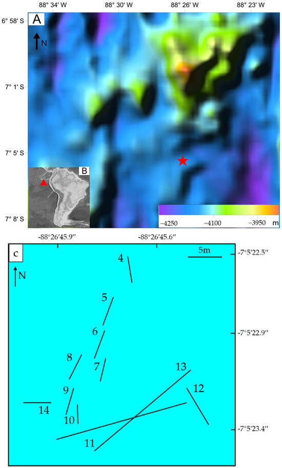
Figure 1.
(A) Bathymetric map (500 m resolution, from GEBCO), with red star marking the location of the study area; (B) overview map of the study area (red triangle) and offshore region of the Peru Basin; and (C) locations of the 11 main survey tracks (Tracks 4–14) of this study.
2.2. Data Preprocessing
The raw data were preprocessed using radiometric correction and other preprocessing to reduce the data to 83 bands between 400 and 710 nm, and the data format was BSQ, containing 15 hyperspectral trajectory data, of which 11 trajectories with serial numbers 4–14, which are suitable for polymetallic nodule identification, were selected for further analysis on the basis of the preprocessing results. The UHI pseudo-RGB data consisting of three bands, 645 nm (R), 571 nm (G), and 473 nm (B), were used for identification. The processed pseudo-RGB image is shown in Figure 2a, and the polymetallic nodules presented in the image are characterized as shown in Figure 2b.
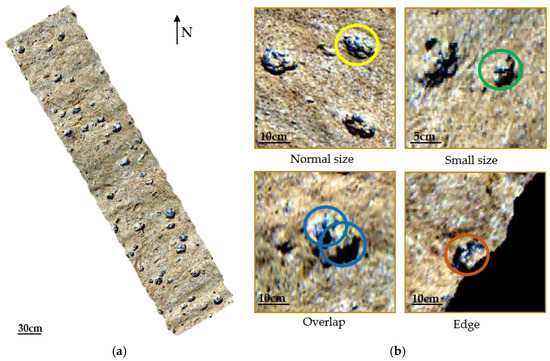
Figure 2.
(a) Processed Pseudo-RGB image and (b) schematic diagram of polymetallic nodule classification.
2.3. Dataset
The images in the dataset contain polymetallic nodules of various shapes and sizes, the dataset size is small, and the imbalance of the actual training data may lead to wrong classifications. Considering this, in this paper, some of the processed images were rotated and cropped for sample expansion, and the dataset was co-produced with a total sample size of 2508 to ensure the performance of model detection. In the dataset, 60% were used for training, 20% for validation, and 20% for testing. The target annotation of image data was performed using LabelImg and the annotation file was stored in txt format. The division of the dataset is shown in Table 1.

Table 1.
Dataset segmentation.
As shown in Figure 2b, the polymetallic nodules in this study can be classified into the following four categories based on the image characteristics: (1) normal-sized nodules (approximately 10 cm in diameter), (2) small-sized nodules (nodules that are partially exposed or visually less than 5 cm in diameter), (3) overlap between two nodules, and (4) nodules that are incomplete at the edge of the image. It should be noted that classification (3) is for cases where there is overlap between the nodules. In some cases, the nodules internally are formed by multiple nucleus (polynucleated) and sometimes formed by de accretion of two of more nodules during growth (polynodules).
3. Methods
3.1. YOLOv5
The basic idea of YOLOv5 is to preprocess the input image into 640 × 640 × 3 matrix data, divide it into N × N grids, judge whether there is a detection target in the grid area according to whether the confidence of each grid exceeds the set threshold, and classify that predicted target according to the classification probability. The precise position and size of the target are then determined by the detected rectangular frame, and, finally, the output result displays the prediction information of each grid.
The network structure of YOLOv5s is shown in Figure 3, which is composed of four parts, including Input, Backbone, Neck and Head [43], and the functions of each part are as follows:
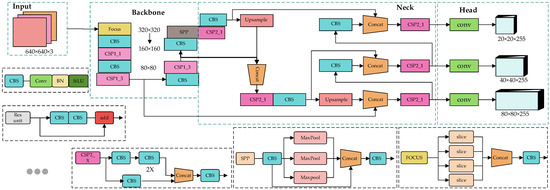
Figure 3.
YOLOv5s network structure.
- (1)
- Input: the input image is preprocessed so that the size of the picture becomes 640 × 640 × 3 and the image data is normalized.
- (2)
- Backbone: focus structure is used as a benchmark network, combined with CSP structure, to extract image data features.
- (3)
- Neck: FPN + PAN structure is used to further fuse and extract the information output by Backbone.
- (4)
- Head: GIOU Loss is used as a loss function to process the characteristic information output by the Neck and output a detection result.
There are 5 versions of YOLOv5 detection network, including YOLOv5s, YOLOv5m, YOLov5l, YOLOv5x, and YOLOv5n. The difference between these is that the number of convolution kernels used in the Focus structure is different. The reason for choosing YOLOv5s in this paper is that it takes into account both the accuracy and complexity of the model, with small size and fast speed [43].
3.2. Detection Mechanism
IoU represents the Intersection over Union, and its simplified mathematical equation is , as shown in Figure 4. Calculating the intersection of two rectangular boxes A and B is essentially calculating the intersection of two sets (A, B), which is further simplified to the calculation of the upper and lower boundary point of the intersection. The role of IoU is to determine positive and negative samples and calculate the non-maximum suppression value (NMS). It can be found from Figure 5 that, for small targets, slight position deviation will cause obvious changes in IoU. There will also be some changes to normal-size targets. Therefore, new metrics need to be introduced in small-target detection to measure the similarity between different distributions, so as to achieve better results in small-target detection.
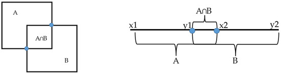
Figure 4.
IoU geometric diagram.
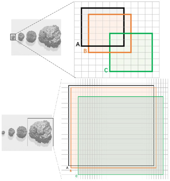
Figure 5.
IoU sensitivity analysis diagram of small targets and normal-scale targets (each grid represents one pixel, box A represents the true bounding box, and boxes B and C represent the predicted bounding boxes with diagonal deviations of 1 and 4 pixels, respectively).
Small targets often have partial background pixels in their rectangular boxes, in which the foreground and background pixels are concentrated in the center and boundary of the rectangular box, respectively [46]. The rectangular box is modeled as a two-dimensional Gaussian distribution to better describe the weights of different pixels in the rectangular box, where the weight of the central pixel in the rectangular box is the highest and the weight of the pixel decreases from the center to the boundary. Converted into a mathematical model, the rectangular box can be modeled as a two-dimensional Gaussian distribution
where w and h represent the center coordinates, width and height, respectively. μ and Σ represent the covariance matrix of the mean vector and Gaussian distribution. Furthermore, the distribution distance between the two Gaussian distributions is used to measure the similarity between the two rectangular boxes.
The Wasserstein distance comes from the distance metric in Optimal Transport theory. The second-order Wasserstein distance between two two-dimensional Gaussian distributions and , and is defined as
It can be simplified as:
where is the Frobenius norm. For Gaussian distributions and modeled by rectangular boxes and , this can be further simplified to
A value using the exponential form normalization of the distance metric as a metric to measure similarity is called the Normalized Wasserstein distance (NWD)
In the equation, C is a constant related to the data set. In this paper, C is set to the average absolute size of the Tiny Object Detection Dataset (AI-TOD). The loss function is set via the NWD indicator as follows: . Among them, and are the Gaussian distributions of the prediction boxes P and G, respectively. As shown in Figure 6a, the NWD-based loss can provide gradients in both cases with and .
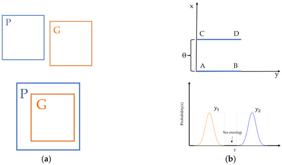
Figure 6.
Schematic diagram of NWD reflecting the distance of the prediction box; (a) P is the prediction box, G is the real frame, and (b) NWD reflects Gaussian distribution distance diagram.
As shown in Figure 6b, P1 and P2 are two distributions in two-dimensional space. P1 and P2 are evenly distributed on the line segments AB and CD, respectively. By adjusting the parameter θ, the distance between two distributions can be controlled. Similarly, in a multidimensional space, with the distribution of two overlapping parts that can be ignored or do not overlap, θ can provide effective measurement references; that is, NWD can effectively measure the distance between two distributions. NWD has the following advantages in small object detection: (1) the metric scale remains unchanged, (2) it can effectively handle positional deviations, and (3) it can measure the similarity between non-overlapping or mutually contained rectangular boxes. Also, it has good generalization in small-target recognition in different scenarios [40].
Based on plenty of previous experiments, we found that the original YOLOv5s reference network failed to achieve the expected recognition effect. Considering that the image contains some small-scale polymetallic nodules and occluded parts that are difficult to accurately recognize, according to the characteristics of NWD in small object detection, NWD is integrated into the original network to replace IoU, and the original part of the original network that used IoU is modified, including NMS (Non-Maximum Suppression) and loss function. Additionally, a small-target recognition method that integrates IoU and NWD metrics is proposed, allowing IoU and NWD to participate in the network structure to certain proportions to improve the performance of the model in the recognition of polymetallic nodules.
Based on the above analysis, the basic process of polymetallic nodule identification using the improved method is shown in Figure 7.
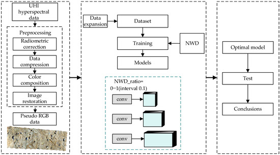
Figure 7.
Workflow of polymetallic nodule identification.
3.3. Workflow
- (1)
- Preprocess original data, including radiation correction, data compression, color synthesis and image enhancement, to obtain processed image data.
- (2)
- Divide the polymetallic nodules in the image into four categories according to the characteristics of the image, adding network public data to expand the number of samples, making a data set together with the processed image data, and divide the data set into a training set, a verification set and a test set according to a ratio of 6:2:2.
- (3)
- With YOLOv5s as the benchmark network, the NWD metric is integrated into the network to participate in the identification work together with the IoU metric in the benchmark network. Five models with different NWD fusion ratios were set up to conduct ablation experiments to test the influence of different fusion ratios of the two metrics on the model recognition effect.
- (4)
- Carrying out an experiment on the test set, comparing a recognition result with a manually marked true value result, counting the correct number, the false test number, and the missed test number of each model, and calculating performance indexes such as precision rate, Recall rate, and the like.
- (5)
- Comparing various evaluation indexes and finally obtaining an optimal model for recognizing the polymetallic nodules by taking YOLOv5s as a reference network and fusing two detection modes of IoU and NWD.
4. Results
4.1. Platform and Indicators
This experiment was built based on the deep learning framework Pytorch. The experimental environment configuration is shown in Table 2.
Table 2.
Experimental environment.
The following four commonly used indicators in the field of object detection are used to measure the performance of the model: precision, recall, mAP and box_loss.
Precision refers to the proportion of correctly predicted positive examples to all predicted positive examples. Recall refers to the proportion of correctly predicted positive examples to all actual positive examples, mAP refers to the average value of all precisions, and box_loss is the error between the prediction box and the calibration box
where TP (True Positive) means that the predicted positive example is actually a positive example; FN (False Negative) means that the predicted positive example is actually a negative example; FP (False Positive) means that the predicted negative example is actually a positive example; AP means the average accuracy of a single category; and mAP is the average of all accuracy
where N represents the number of detected target categories.
4.2. Ablation Experiment
According to the actual situation, ten improved models with different fusion ratios (the range is 0–1, and the interval is 0.1) were set for ablation experiments, and five models with the most obvious change characteristics were selected according to the experimental results. The fusion ratios of each model were 0, 0.3, 0.5, 0.8, and 1, respectively. After the training set and validation set experiments, the precision, recall, average precision, and loss curves of the model were calculated and are shown in Figure 8, where, the horizontal axis is the training period, the vertical axis is the model performance index, and the NWD_ratio is the NWD fusion ratio of the model. It can be seen that in the training process, when the NWD_ratio is 0.5, the model accuracy is the highest, which is significantly improved compared with the original model without NWD. At the same time, it can be found that the performance of each model is different due to the difference in NWD fusion ratio. When the NWD_ratio is 1, that is, the IoU metric in the original model is completely replaced, the accuracy of the model is reduced. Similarly, when the NWD_ratio is 0.5 the model has the highest recall, which is significantly higher than that of the original model. With the gradual increase in the NWD fusion ratio, the recall also changes. When the NWD_ratio is 0.5, the model has a smaller loss value and faster convergence speed than other models, indicating that the error between the prediction frame and the calibration frame is smaller, and the mAP is higher than that of other models. Therefore, the model with an NWD fusion ratio of 0.5 is taken as the optimal model for improvement, that is, the ratio of NWD and IoU in the improved network is 0.5, respectively.
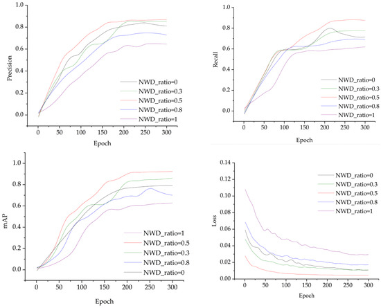
Figure 8.
Performance results of models with different NWD fusion ratios.
Figure 9 shows the performance results of different improved models. By comparison, it can be found that the model effect is a follows: NWD_ratio = 0.5 > NWD_ratio = 0.3 > NWD_ratio = 0 > NWD_ratio = 0.8 > NWD_ratio = 1. The specific test results are shown in Table 3. When the NWD fusion ratio is 0.5, the model performs best, where the accuracy is 6.2% higher than that of the original network, the mAP@0.5 is 13.4% higher than that of the original network, and the recall is 16% better than that of the original model. It can be seen from the figure that the performance of the model changes greatly with the change in the NWD fusion ratio. When the NWD fusion ratio gradually increases from 0, the performance of the model is significantly improved. When the NWD fusion ratio exceeds 0.5, the performance is significantly reduced and is lower than that of the original network. In this experiment, the complete replacement of IoU detection in the original network by NWD does not give the best results. After analysis, not all polymetallic nodules in the image belong to small-target detection, and the excessive proportion of NWD will lead to multiple rectangular frames of the same target in the recognition results. Therefore, we take the NWD_ratio of the improved scheme = 0.5 as the final improved model.
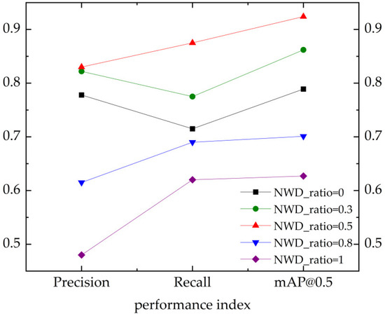
Figure 9.
Comparison of performance results of different improved models.
Table 3.
Statistics of detection results of different improved models.
4.3. Variance Analysis
542 samples in the test set are recognized, and the recognition results of different improved models are shown in Figure 10. When the NWD_ratio is 0.5, the small-sized polymetallic nodules partially exposed out of seabed sediments and the nodules located at the edge of the image can be accurately recognized, and the problem of repeated detection frames does not occur for small-sized targets. The coincidence degree with the artificial marking result is the highest, and the recognition effect is the best. The original network model without NWD has the problems of missed detection and false detection, which cannot accurately identify some smaller polymetallic nodules, and there is confusion between polymetallic nodules and sediment protuberances. When the NWD_ratio is 1, there are many repeated detection frames in the same target recognition result for the small-size polymetallic nodules, and the number of missed detection and false detection increases.
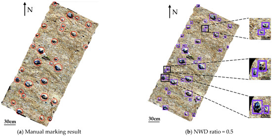
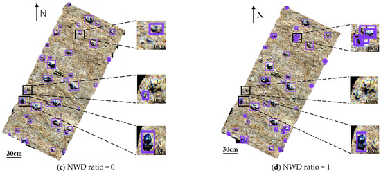
Figure 10.
Recognition results of different improved models.
For each model, the block count, the number of correct detection, the number of false detection, and the number of missed detection are shown in Table 4. According to the statistical results, the number of missed detection and false detection is the least when NWD_ratio is 0.5, with the number of missed detections reduced by more than half and the number of false detection reduced by about one third compared with the original model without NWD. When the NWD_ratio is 0.5, the precision and recall of the model are the highest. When the NWD_ratio is 0.3, there is no significant change in the number of correct tests, the number of false tests is reduced, and the number of tiles is reduced, so the precision and recall are partially improved compared with the network without NWD. When the NWD_ ratio is 0.8, the correct number, the number of image blocks and the number of errors are significantly increased compared with when the NWD_ratio is 0.5, resulting in a decrease in accuracy. When the NWD_ratio is 1, the model has the largest number of tile counts and detections, and the accuracy rate decreases, which is in line with the model performance results. To sum up, the model with the fusion ratio of NWD and IoU of 0.5 is taken as the final improved model in this study.
Table 4.
Test set statistics results.
5. Discussion
In our model, the NWD metric was introduced to replace the NMS in the original network and the IoU part of the loss function. Ten different fusion ratios ranging from 0–1 (five with obvious changes were selected in the paper) were set for the ablation experiments, and the model performance was further evaluated using four indicators including precision, recall, loss, and mean average precision. By adjusting the NWD fusion ratios, the optimal ratio of IoU and NWD metric fusion was found, and the improved model with better recognition was thus obtained. The experimental results show that the number of correct recognitions was closest to that of manual markers, with the fewest number of false and missed detections, and the precision rate was improved by 6.2% compared to the original model when the ratio of NWD and IoU fusion was 0.5. All evaluation metrics are significantly improved over the original model.
The improved model has better recognition of small-sized polymetallic nodules and semi-buried metallic nodules in data classification, achieving what we expected. Small-sized and semi-buried polymetallic nodules are of great significance in seafloor-mineral- resource exploration, and it is likely that a significant portion of them remain unrevealed under sediment cover [59,60,61]. We also found that, when the fusion ratio of NWD was more than 0.5, the model recognition effect was deeply affected by the duplicate detection frame, as both precision rate and recall rate were decreased. This is mainly because IoU is the ratio of the intersection and concatenation of the two bounding boxes, and a larger value of IoU indicates that the two boxes are closer. The NMS (Non-Maximum Suppression) algorithm is used in the YOLO model to deal with the problem of targets being detected multiple times [62]. The NMS selects the detection frame with the highest confidence from all of the frames and then calculates the IoU of the remaining detection frames with that frame. If the IoU is greater than the threshold set, it means that there is too much overlap between the two boxes, and the box will be removed. The NWD metric is a good measure of the similarity between two small targets and it outperforms traditional metrics for target identification in tests on public datasets [63].
The NWD metric cannot completely replace IoU in this model, and after experiments, we set a scaling parameter so that the two metrics can jointly participate in the deep-sea polymetallic nodule-identification process. In subsequent larger datasets of polymetallic nodules, this scaling parameter will need to be adjusted so that the two metrics can still work in tandem to achieve the best possible identification.
6. Conclusions
In order to more effectively utilize deep-sea hyperspectral data for the exploration of polymetallic nodule resources, this paper proposes a polymetallic nodule-identification method based on the YOLOv5s network, which integrates two indicators, NWD and IoU. The method fully considers the characteristics of high-resolution hyperspectral data and applies them to deep-sea polymetallic nodule resource investigations. We selected the hyperspectral remote sensing images obtained by the Underwater Hyperspectral Imager in the Peru Basin of the Southeast Pacific Ocean as the experimental data, classified the polymetallic nodules according to their sizes and burial conditions, introduced the NWD metric to replace the NMS (non-maximum suppression) in the original network and the IoU part in the loss function, and tested the efficiency of the different improved models in recognizing the polymetallic nodules through the adjustment of the fusion ratio of the NWD to find a more suitable method for recognizing small-sized and partial polymetallic nodules.
The method proposed in this paper has a beneficial effect on recognizing small-sized polymetallic nodules and partially buried nodules, and it can be applied to the exploration of deep-sea mineral resources. It should be noted that, in many cases, most of the small or half-buried polymetallic nodules in the image cannot be visualized in the image under the cover of sediment (these nodules play an important role in the development and utilization of deep-sea-mineral resources), so the question of how to more accurately identify this type of nodules needs our further research.
The importance of this methodology is not only for detecting big nodules, but also the small ones, contributing in a better way to estimating the percentage of seafloor-coverage from nodules. On occasion, these apparently small nodules are partially buried, which has implications for mining and geological studies. It is interesting to consider the application of these methods to vast areas of abyssal plains providing predictive models and mapping for future exploration of resources.
Author Contributions
Conceptualization, K.S., Z.L., D.Z., J.S. and X.L.; Methodology, K.S. and M.W.; Validation, Z.W. and M.W.; Resources, Z.W. and M.W.; Data curation, M.W.; Writing—original draft, K.S., Z.W., M.W. and Z.L.; Writing—review and editing, D.Z., J.S. and X.L.; Visualization, K.S.; Supervision, Z.W. and M.W. All authors have read and agreed to the published version of the manuscript.
Funding
This study is supported by the National Key Research and Development Program of China (2022YFC2806600), the National Natural Science Foundation of China (41830540), Fundamental Research Funds for Central Public Welfare Research Institutes of China (JG2205), the Open Fund of Key Laboratory Seafloor Science, the Ministry of Natural Resources (KLSG2203), and the Oceanic Interdisciplinary Program of Shanghai Jiao Tong University (SL2020ZD204, SL2020ZD205).
Institutional Review Board Statement
Not applicable.
Informed Consent Statement
Not applicable.
Data Availability Statement
The authors would like to express their gratitude to PANGAEA (https://www.pangaea.de/, accessed on 20 April 2023) for UHI Data services and Jinwang Wang for uploading the code of the NWD Models onto GitHub (https://github.com/jwwangchn/NWD, accessed on 20 April 2023).
Conflicts of Interest
The authors declare no conflicts of interest.
References
- Wu, Z.; Yang, F.; Tang, Y. High-Resolution Seafloor Survey and Applications; Science Press: Beijing, China, 2021. [Google Scholar]
- Hein, J.R.; Koschinsky, A.; Kuhn, T. Deep-ocean polymetallic nodules as a resource for critical materials. Nat. Rev. Earth Environ. 2020, 1, 158–169. [Google Scholar] [CrossRef]
- Kuhn, T.; Wegorzewski, A.; Rühlemann, C.; Vink, A. Composition, formation, and occurrence of polymetallic nodules. In Deep-Sea Mining: Resource Potential, Technical and Environmental Considerations; Springer: Cham, Switzerland, 2017; pp. 23–63. [Google Scholar]
- Wang, X.; Müller, W.E.G. Marine biominerals: Perspectives and challenges for polymetallic nodules and crusts. Trends Biotechnol. 2009, 27, 375–383. [Google Scholar] [CrossRef]
- Kang, Y.; Liu, S. The development history and latest progress of deep-sea polymetallic nodule mining technology. Minerals 2021, 11, 1132. [Google Scholar] [CrossRef]
- Abramowski, T.; Stoyanova, V. Deep-sea polymetallic nodules: Renewed interest as resources for environmentally sustainable development. In Proceedings of the 12th International Multididciplinary Scientific GeoConference: SGEM, Surveying Geology and Mining Ecology Management, Varna, Bulgaria, 17–23 June 2012; Volume 1, pp. 515–521. [Google Scholar]
- Thomson, C.W.; Murray, J. Report on the Scientific Results of the Voyage of H.M.S. Challenger during the Years 1872–76; Her Majesty’s Government: Edinburgh, UK, 1895.
- Kuhn, T.; Rühlemann, C.; Wiedicke-Hombach, M. Developing a Strategy for the Exploration of Vast Seafloor Areas for Prospective Manganese Nodule Fields. In Proceedings of the 41st Conference of the Underwater Mining Institute, UMI 2012, Shanghai, China, 15–20 October 2012. [Google Scholar]
- Halbach, P.; Kriete, C.; Prause, B.; Puteanus, D. Mechanisms to explain the platinum concentration in ferromanganese seamount crusts. Chem. Geol. 1989, 76, 95–106. [Google Scholar] [CrossRef]
- Hein, J.R.; Mizell, K.; Koschinsky, A.; Conrad, T.A. Deep-ocean mineral deposits as a source of critical metals for high- and green-technology applications: Comparison with land-based resources. Ore Geol. Rev. 2013, 51, 1–14. [Google Scholar] [CrossRef]
- Koschinsky, A.; Hein, J.R.; Kraemer, D.; Foster, A.L.; Kuhn, T.; Halbach, P. Platinum enrichment and phase associations in marine ferromanganese crusts and nodules based on a multi-method approach. Chem. Geol. 2020, 539, 119426. [Google Scholar] [CrossRef]
- Lusty, P.A.J.; Hein, J.R.; Josso, P. Formation and Occurrence of Ferromanganese Crusts: Earth’s Storehouse for critical Metals. Elements 2018, 14, 313–318. [Google Scholar] [CrossRef]
- Nozaki, T.; Tokumaru, A.; Takaya, Y.; Kato, Y.; Urabe, T. Major and trace element compositions and resource potential of ferromanganese crust at Takuyo Daigo Seamount, northwestern Pacific Ocean. Geochem. J. 2016, 50, 527–537. [Google Scholar] [CrossRef]
- Knobloch, A.; Kuhn, T.; Rühlemann, C.; Hertwig, T.; Zeissler, K.-O.; Noack, S. Predictive Mapping of the Nodule Abundance and Mineral Resource Estimation in the Clarion-Clipperton Zone Using Artificial Neural Networks and Classical Geostatistical Methods. In Deep-Sea Mining; Sharma, R., Ed.; Springer International Publishing: Cham, Switzerland, 2017; Volume 122, pp. 189–212. [Google Scholar]
- Sakellariadou, F.; Gonzalez, F.J.; Hein, J.R.; Rincón-Tomás, B.; Arvanitidis, N.; Kuhn, T. Seabed mining and blue growth: Exploring the potential of marine mineral deposits as a sustainable source of rare earth elements (MaREEs) (IUPAC Technical Report). Pure Appl. Chem. 2022, 94, 329–351. [Google Scholar] [CrossRef]
- González, F.J.; Medialdea, T.; Schiellerup, H.; Zananiri, I.; Ferreira, P.; Somoza, L.; Monteys, X.; Alcorn, T.; Marino, E.; Lobato, A.B.; et al. MINDeSEA: Exploring seabed mineral deposits in European seas, metallogeny and geological potential for strategic and critical raw materials. Geol. Soc. Lond. Spec. Publ. 2023, 526, 289–317. [Google Scholar] [CrossRef]
- Marino, E.; González, F.J.; Kuhn, T.; Madureira, P.; Somoza, L.; Medialdea, T.; Lobato, A.; Miguel, C.; Reyes, J.; Oeser, M. Factors controlling rare earth element plus yttrium enrichment in FeMn crusts from Canary Islands Seamounts (NE Central Atlantic). Mar. Geol. 2023, 464, 107144. [Google Scholar] [CrossRef]
- Joo, J.; Kim, S.S.; Choi, J.W.; Pak, S.J.; Ko, Y.; Son, S.K.; Moon, J.; Kim, J. Seabed mapping using shipboard multibeam acoustic data for assessing the spatial distribution of ferromanganese crusts on seamounts in the western pacific. Minerals 2020, 10, 155. [Google Scholar] [CrossRef]
- Qin, X.; Wu, Z.; Luo, X.; Li, B.; Zhao, D.; Zhou, J.; Wang, M.; Wan, H.; Chen, X. Temporal Fusion Based 1-D Sequence Semantic Segmentation Model for Automatic Precision Side Scan Sonar Bottom Tracking. IEEE Trans. Geosci. Remote Sens. 2023, 61, 4201816. [Google Scholar] [CrossRef]
- Kuhn, T.; Rühlemann, C. Exploration of polymetallic nodules and resource assessment: A case study from the German contract area in the Clarion-Clipperton Zone of the tropical Northeast Pacific. Minerals 2021, 11, 618. [Google Scholar] [CrossRef]
- Wang, M.; Wu, Z.; Zhang, K.; Zhao, D.; Zhou, J.; Luo, X.; Shang, J.; Liu, Y.; Sun, K. Mixed Seabed Sediment Classification Based on Transferred Convolutional Neural Network: A Case Study in the Ancient River Valley. IEEE Trans. Geosci. Remote Sens. 2023, 61, 4205116. [Google Scholar] [CrossRef]
- Kuhn, T.; Rathke, M. Visual Data Acquisition in the Field and Interpretation for Seafloor Manganese Nodules. EU Project Blue Mining (GA No. 604500) Delivery D1.31. 2017; p. 34. Available online: https://www.bluemining.eu/downloads (accessed on 14 June 2019).
- Tao, C.; Jin, X.; Bain, A.; Li, H.; Deng, X.; Zhou, J.; Gu, C.; Wu, T.; Roy, W. Estimation of manganese nodule coverage using multi-beam amplitude data. Mar. Georesour. Geotechnol. 2015, 33, 283–288. [Google Scholar]
- Chennu, A.; Färber, P.; Volkenborn, N.; Al-Najjar, M.A.; Janssen, F.; De Beer, D.; Polerecky, L. Hyperspectral imaging of the microscale distribution and dynamics of microphytobenthos in intertidal sediments. Limnol. Oceanogr. Methods 2013, 11, 511–528. [Google Scholar] [CrossRef]
- Johnsen, G.; Volent, Z.; Dierssen, H.; Pettersen, R.; Ardelan, M.V.; Søreide, F.; Fearns, P.; Ludvigsen, M.; Moline, M. Underwater Hyperspectral Imagery to Create Biogeochemical Maps of Seafloor Properties Subsea Optics and Imaging; Woodhead Publishing: Sawston, UK, 2013; pp. 508–540e. [Google Scholar]
- Tegdan, J.; Ekehaug, S.; Hansen, I.M.; Aas, L.M.; Steen, K.J.; Pettersen, R.; Beuchel, F.; Camus, L. Underwater Hyperspectral Imaging for Environmental Mapping and Monitoring of Seabed Habitats OCEANS 2015-Genova; IEEE: Genoa, Italy, 2015; pp. 1–6. [Google Scholar]
- Sture, Ø.; Ludvigsen, M.; Aas, L.M.S. Autonomous Underwater Vehicles as a Platform for Underwater Hyperspectral Imaging Oceans 2017-Aberdeen; IEEE: Aberdeen, UK, 2017; pp. 1–8. [Google Scholar]
- Van der Meer, F.D.; Van der Werff, H.M.A.; Van Ruitenbeek, F.J.A.; Hecker, C.A.; Bakker, W.H.; Noomen, M.F.; van der Meijde, M.; Carranza, E.J.M. Boudewijn de Smeth, Tsehaie Woldai. Multi-and hyperspectral geologic remote sensing: A review. Int. J. Appl. Earth Obs. Geoinf. 2012, 14, 112–128. [Google Scholar]
- Dumke, I.; Purser, A.; Marcon, Y.; Nornes, S.M.; Johnsen, G.; Ludvigsen, M.; Søreide, F. Underwater hyperspectral imaging as an in situ taxonomic tool for deep-sea megafauna. Sci. Rep. 2018, 8, 12860. [Google Scholar] [CrossRef]
- Dumke, I.; Nornes, S.M.; Purser, A.; Marcon, Y.; Ludvigsen, M.; Ellefmo, S.L.; Johnsen, G.; Søreide, F. First hyperspectral imaging survey of the deep seafloor: High-resolution mapping of manganese nodules. Remote Sens. Environ. 2018, 209, 19–30. [Google Scholar] [CrossRef]
- Sun, H.; Zheng, X.; Lu, X. A supervised segmentation network for hyperspectral image classification. IEEE Trans. Image Process. 2021, 30, 2810–2825. [Google Scholar] [CrossRef]
- Liu, B.; Yu, X.; Zhang, P.; Yu, A.; Fu, Q.; Wei, X. Supervised deep feature extraction for hyperspectral image classification. IEEE Trans. Geosci. Remote Sens. 2017, 56, 1909–1921. [Google Scholar] [CrossRef]
- Lv, W.; Wang, X. Overview of hyperspectral image classification. J. Sens. 2020, 2020, 4817234. [Google Scholar] [CrossRef]
- Bilgin, G.; Erturk, S.; Yildirim, T. Unsupervised classification of hyperspectral-image data using fuzzy approaches that spatially exploit membership relations. IEEE Geosci. Remote Sens. Lett. 2008, 5, 673–677. [Google Scholar] [CrossRef]
- Abid, N.; Shahzad, M.; Malik, M.I.; Schwanecke, U.; Ulges, A.; Kovács, G.; Shafait, F. UCL: Unsupervised Curriculum Learning for water body classification from remote sensing imagery. Int. J. Appl. Earth Obs. Geoinf. 2021, 105, 102568. [Google Scholar] [CrossRef]
- Fang, H.; Du, P.; Wang, X. A novel unsupervised binary change detection method for VHR optical remote sensing imagery over urban areas. Int. J. Appl. Earth Obs. Geoinf. 2022, 108, 102749. [Google Scholar] [CrossRef]
- Ye, P.; Han, C.; Zhang, Q.; Gao, F.; Yang, Z.; Wu, G. An Application of Hyperspectral Image Clustering Based on Texture-Aware Superpixel Technique in Deep Sea. Remote Sens. 2022, 14, 5047. [Google Scholar] [CrossRef]
- Wang, J.; Yang, W.; Li, H.-C.; Zhang, H.; Xia, G.-S. Learning center probability map for detecting objects in aerial images. IEEE Trans. Geosci. Remote Sens. 2020, 59, 4307–4323. [Google Scholar] [CrossRef]
- Kisantal, M.; Wojna, Z.; Murawski, J.; Naruniec, J.; Cho, K. Augmentation for small object detection. arXiv 2019, arXiv:1902.07296. [Google Scholar]
- Bodla, N.; Singh, B.; Chellappa, R.; Davis, L.S. Soft-NMS—Improving object detection with one line of code. In Proceedings of the IEEE International Conference on Computer Vision, Venice, Italy, 22–29 October 2017; pp. 5561–5569. [Google Scholar]
- Eggert, C.; Brehm, S.; Winschel, A.; Zecha, D.; Lienhart, R. A closer look: Small object detection in faster R-CNN. In Proceedings of the 2017 IEEE International Conference on Multimedia and Expo (ICME), Hong Kong, China, 10–14 July 2017; pp. 421–426. [Google Scholar]
- Ren, Y.; Zhu, C.; Xiao, S. Small object detection in optical remote sensing images via modified faster R-CNN. Appl. Sci. 2018, 8, 813. [Google Scholar] [CrossRef]
- Jocher, G.; Nishimura, K.; Mineeva, T. YOLOv5 (Minor Version 6.0) [EB/OL]. Available online: https://github.com/ultralytics/yolov5/releases/tag/v6.0 (accessed on 1 May 2023).
- Panaretos, V.M.; Zemel, Y. Statistical aspects of Wasserstein distances. Annu. Rev. Stat. Its Appl. 2019, 6, 405–431. [Google Scholar] [CrossRef]
- Yu, J.; Jiang, Y.; Wang, Z.; Cao, Z.; Huang, T. Unitbox: An advanced object detection network. In Proceedings of the 24th ACM International Conference on Multimedia, Amsterdam, The Netherlands, 15–19 October 2016; pp. 516–520. [Google Scholar]
- Wang, J.; Xu, C.; Yang, W.; Yu, L. A normalized Gaussian Wasserstein distance for tiny object detection. arXiv 2021, arXiv:2110.13389. [Google Scholar]
- Von Stackelberg, U. Growth history of manganese nodules and crusts of the Peru Basin. Geol. Soc. Lond. Spec. Publ. 1997, 119, 153–176. [Google Scholar] [CrossRef]
- Thornburg, T.M.; Kulm, L.D. Sedimentary basins of the Peru continental margin: Structure, stratigraphy, and Cenozoic tectonics from 6 S to 16 S latitude. Nazca Plate Crustal Form. Andean Converg. 1981, 154, 393–422. [Google Scholar]
- Weber, M.E.; Wiedicke, M.; Riech, V.; Erlenkeuser, H. Carbonate preservation history in the Peru Basin: Paleoceanographic implications. Paleoceanography 1995, 10, 775–800. [Google Scholar] [CrossRef]
- Thiel, H. Use and protection of the deep sea-an introduction. Deep-Sea Res. Part II Top. Stud. Oceanogr. 2001, 48, 3427–3431. [Google Scholar] [CrossRef]
- Devey, C.W.; Greinert, J.; Boetius, A.; Augustin, N.; Yeo, I. How volcanically active is an abyssal plain II Evidence for recent volcanism on 20 Ma Nazca Plate seafloor. Mar. Geol. 2021, 440, 106548. [Google Scholar] [CrossRef]
- Borowski, C. Physically disturbed deep-sea macrofauna in the Peru Basin, south-east Pacific, revisited 7 years after the experimental impact. Deep-Sea Res. II 2001, 48, 3809–3839. [Google Scholar] [CrossRef]
- Haeckel, M.; König, I.; Riech, V.; Weber, M.E.; Suess, E. Pore water profiles and numerical modelling of biogeochemical processes in Peru Basin deep-sea sediments. Deep. Sea Res. Part II Top. Stud. Oceanogr. 2001, 48, 3713–3736. [Google Scholar] [CrossRef]
- Grupe, B.; Becker, H.J.; Oebius, H.U. Geotechnical and sedimentological investigations of deep-sea sediments from a manganese nodule field of the Peru Basin. Deep. Sea Res. Part II Top. Stud. Oceanogr. 2001, 48, 3593–3608. [Google Scholar] [CrossRef]
- Weber, M.; von Stackelberg, U.; Marchig, V.; Wiedicke, M.; Grupe, B. Variability of surface sediments in the Peru basin: Dependence on water depth, productivity, bottom water flow, and seafloor topography. Mar. Geol. 2000, 163, 169–184. [Google Scholar] [CrossRef]
- Von Stackelberg, U. Manganese Nodules of the Peru Basin Handbook of Marine Mineral Deposits; Routledge: London, UK, 2017; pp. 197–238. [Google Scholar]
- Borowski, C.; Thiel, H. Deep-sea macrofaunal impacts of a large-scale physical disturbance experiment in the Southeast Pacific. Deep-Sea Res. II 1998, 45, 55–81. [Google Scholar] [CrossRef]
- Greinert, J. RV SONNE Fahrtbericht/Cruise Report SO242-1 [SO242/1]: JPI OCEANS Ecological Aspects of Deep-Sea Mining, DISCOL Revisited, Guayaquil-Guayaquil (Equador), 28.07.–25.08. 2015; GEOMAR Helmholtz-Zentrum für Ozeanforschung: Kiel, Germany, 2015. [Google Scholar]
- Tsune, A.; Okazaki, M. Some Considerations about Image Analysis of Seafloor Photographs for Better Estimation of Parameters of Polymetallic Nodule Distribution. In Proceedings of the ISOPE International Ocean and Polar Engineering Conference, ISOPE, Busan, Republic of Korea, 15–20 June 2014. ISOPE-I-14-117. [Google Scholar]
- Gazis, I.Z.; Schoening, T.; Alevizos, E.; Greinert, J. Quantitative map** and predictive modeling of Mn nodules’ distribution from hydroacoustic and optical AUV data linked by random forests machine learning. Biogeosciences 2018, 15, 7347–7377. [Google Scholar] [CrossRef]
- Yang, Y.; He, G.; Ma, J.; Yu, Z.; Yao, H.; Deng, X.; Liu, F.; Wei, Z. Acoustic quantitative analysis of ferromanganese nodules and cobalt-rich crusts distribution areas using EM122 multibeam backscatter data from deep-sea basin to seamount in Western Pacific Ocean. Deep Sea Res. Part I Oceanogr. Res. Pap. 2020, 161, 103281. [Google Scholar] [CrossRef]
- Neubeck, A.; Gool, L.J.V. Efficient Non-Maximum Suppression. In Proceedings of the 18th International Conference on Pattern Recognition (ICPR 2006), Hong Kong, China, 20–24 August 2006. [Google Scholar]
- Zhang, J.; Wei, X.; Zhang, L.; Yu, L.; Chen, Y.; Tu, M. YOLO v7-ECA-PConv-NWD Detects Defective Insulators on Transmission Lines. Electronics 2023, 12, 3969. [Google Scholar] [CrossRef]
Disclaimer/Publisher’s Note: The statements, opinions and data contained in all publications are solely those of the individual author(s) and contributor(s) and not of MDPI and/or the editor(s). MDPI and/or the editor(s) disclaim responsibility for any injury to people or property resulting from any ideas, methods, instructions or products referred to in the content. |
© 2024 by the authors. Licensee MDPI, Basel, Switzerland. This article is an open access article distributed under the terms and conditions of the Creative Commons Attribution (CC BY) license (https://creativecommons.org/licenses/by/4.0/).