Abstract
Semantic segmentation methods have been successfully applied in seabed sediment detection. However, fast models like YOLO only produce rough segmentation boundaries (rectangles), while precise models like U-Net require too much time. In order to achieve fast and precise semantic segmentation results, this paper introduces a novel model called YOLO-C. It utilizes the full-resolution classification features of the semantic segmentation algorithm to generate more accurate regions of interest, enabling rapid separation of potential targets and achieving region-based partitioning and precise object boundaries. YOLO-C surpasses existing methods in terms of accuracy and detection scope. Compared to U-Net, it achieves an impressive 15.17% improvement in mean pixel accuracy (mPA). With a processing speed of 98 frames per second, YOLO-C meets the requirements of real-time detection and provides accurate size estimation through segmentation. Furthermore, it achieves a mean average precision (mAP) of 58.94% and a mean intersection over union (mIoU) of 70.36%, outperforming industry-standard algorithms such as YOLOX. Because of the good performance in both rapid processing and high precision, YOLO-C can be effectively utilized in real-time seabed exploration tasks.
1. Introduction
Understanding marine terrain and geomorphology is crucial for gaining comprehensive knowledge of the ocean and effectively exploring and utilizing its resources. A key aspect of marine development involves the identification of seabed sediments. While traditional sediment sampling serves as a fundamental method for seabed sediment classification, various marine acoustic techniques, such as side-scan sonar (SSS), multi-beam echo sounding, and profile sonar sounder, offer alternative means to obtain seabed sediment imagery. However, manual analysis of such imagery is time-consuming and labor-intensive, prompting the development of automatic methods.
Seabed sediment recognition using underwater acoustic detection techniques has emerged as a significant research area. Side-scan sonar systems, operating as active sonars, enable the generation of seabed terrain and geomorphology images. To address the limitations of current seabed sediment detection methods, which often lack precision and have a limited detection scope, we propose an automatic and accurate model called YOLO-C. This model integrates object detection and semantic segmentation techniques to achieve high accuracy and efficiency in detecting seabed sediments from SSS imagery. By combining these approaches, YOLO-C overcomes the imprecise detection outcomes typically associated with methods that only identify rectangular shapes. With its precise boundaries and high precision, YOLO-C aims to enhance the automated recognition of seabed sediments.
Furthermore, the proposed YOLO-C model exhibits exceptional performance in various application areas, distinguishing it from previous studies. Specifically, in the field of marine resource exploration, YOLO-C has the capability to accurately identify and classify different types of seabed sediments, enabling more effective resource assessment and extraction planning. Additionally, in environmental monitoring and conservation efforts, YOLO-C’s precise boundary detection and segmentation allow for the precise mapping of sensitive marine habitats and the detection of any changes or disturbances. Moreover, in underwater archaeological surveys, YOLO-C’s ability to capture detailed sediment characteristics enhances the identification and preservation of submerged cultural heritage sites. These examples demonstrate the versatility and effectiveness of our proposed model in key application domains.
The main contributions of this paper are listed as follows:
- A model YOLO-C is proposed to detect objects and segment images at the same time based on U-Net and YOLOX, which produces higher accurate detection and segmentation results;
- The proposed YOLO-C can produce more details of the seabed sediment, including accurate shape and area;
- YOLO-C has high time efficiency than usual neural network methods.
2. Related Work
2.1. About Seabed Sediment
Seabed sediment recognition can be regarded as a classification process for different sediment types. Some researchers have utilized clustering methods or other classification methods to achieve accurate seabed recognition. Tegowski [1] used clustering-based classification methods in 2004. They utilized integrated spectral width, the Hausdorff fractional dimension of echo envelope, and backscattered intensity as input for the K-means algorithm with 88% accuracy. Lucieer and Lamarche [2] used fuzzy classification algorithms; they used two fuzzy classification algorithms for seascape classification, where FCM (fully convolutional networks) had significant advantages over crisp/complex classifiers, quantifying uncertainties, and mapping transition zones. In 2011, Lucieer and Lamarche [3] applied FCM to substrate classification in the Cook Strait, New Zealand area, indicating affiliation degree to particular classes but with high uncertainty at boundaries. Lark et al. [4] examined a co-Kriging approach to classify image texture for seabed sediments from in situ sampling points with 70% prediction accuracy. Huvenne et al. [5] used texture classification methods. They found that the GLCM (gray-level co-occurrence matrix) could be used for texture classification instead of traditional visual interpretation [6]. Entropy and homogeneity indices were calculated, and the results made it possible to discriminate between different seabed features on a quantitative basis. Li et al. [7] used spatial interpolation to predict mud content in the southwestern region of Australia, selecting random forest and standard Kriging methods as the most robust ones. Overall, clustering-based methods can quickly obtain classification results but have significant errors in category determination and boundary division. Other classification methods, such as correlation-based and texture classification methods, do not require prior knowledge but have poor interpretability of classification results.
With the growing power of artificial intelligence, machine learning algorithms were successfully applied to seabed sediment recognition. Cui et al. [8] proposed a bi-directional sliding window-based angular response feature extraction method with a K-means clustering algorithm for seabed sediment segmentation. It effectively decomposes deep-sea sediment compositions with high accuracy. Marsh and Brown [9] applied a self-organizing artificial neural network to automatic seabed sediment classification, with self-organizing mapping and competing neural networks providing the most accurate results. Berthold et al. [10] used a convolutional neural network (CNN) to automatically classify seafloor sediment based on SSS images with a prediction accuracy of 83%. Xi et al. [11] proposed an improved BP neural network to classify the SSS imagery of seabed sediment. They utilize the gray covariance matrix method to extract four sorts of seabed sediment texture characteristics and input them into the BP neural network optimized by an improved particle swarm optimization algorithm. SUN et al. [12] used a probabilistic neural network (PNN) for seabed sediment classification based on SSS imagery, with high computational and spatial complexity. Steele [13] proposed an unsupervised segmentation technique for accurate and interpretable seabed imagery mapping. The experiments showed that spatially coherent clustering could significantly increase segmentation accuracy relative to OpenCV K-means and ArcGIS Pro iterative self-organizing (ISO) clustering (up to 15% and 20%, respectively). Qin et al. [14] used CNNs with different depths for small seabed acoustic imagery dataset classification. In their experiments, the best result obtained by fine-tuning ResNet was 3.459%. Zheng et al. [15] proposed a robust and versatile automatic bottom-tracking technique based on semantic segmentation for fast and accurate segmentation of SSS waterfall imagery. The results demonstrated that the proposed method achieves a mean error of 1.1 pixels and a standard deviation of 1.26 pixels for bottom tracking accuracy. Furthermore, the method exhibited resilience to interference factors, ensuring reliable performance in challenging conditions. Chen et al. [16] used the SVM classification method for sonar imagery segmentation of seabed sediments. In the test, the classification accuracy of the three types of samples was above 90%. Especially the test accuracy of sand was above 95%. Machine learning methods have good representation capabilities and classification accuracy but require large amounts of data and computational resources.
Unfortunately, the current methods for detecting seabed sediment are not entirely satisfactory due to their lack of precision and the restricted detection scope. Specifically, most of these methods only detect rectangular shapes, which results in imprecise detection outcomes. To solve the problem, the paper proposes an automatic and accurate model named YOLO-C to detect seabed sediments from SSS imagery, which integrates object detection and semantic segmentation with high precision and accurate boundary.
2.2. About Object Detection
Object detection is an important area of research in computer vision that aims to locate specific objects of interest in images or videos. Early object detection algorithms were primarily based on hand-crafted features and classifiers, such as the Viola–Jones algorithm [17], histogram of oriented gradient (HOG) [18], and deformable parts model (DPM) [19]. However, these algorithms often require significant feature engineering and complex model design and have some limitations in practical applications, such as limited accuracy, high computational complexity, extensive annotation requirements, and sensitivity to illumination and viewpoint changes.
To address these challenges, new approaches such as deep learning-based methods have been developed, showing great promise in achieving state-of-the-art performance in object detection tasks.
The most representative algorithms include YOLO (you only look once) [20,21,22,23,24,25,26,27] and Faster R-CNN (faster region-based convolutional neural network) [28]. YOLO can predict whether an object is present in each grid cell of the input image and simultaneously predict its location and class. Faster R-CNN extracts features from the input image and applies the region proposal network (RPN) to the feature map, then performs classification and regression to achieve object detection.
2.3. About Semantic Segmentation
Traditional semantic segmentation algorithms rely on image segmentation and classifiers based on color, texture, and shape, which often require significant low-level feature extraction and complex model design. Recently, deep learning has made remarkable progress in semantic segmentation tasks. A variety of algorithms have been proposed to achieve state-of-the-art performance, including fully convolutional networks (FCN) [29], U-Net [30], DeepLab [31], and the pyramid scene parsing network (PSPNet) [32]. These algorithms employ different techniques to address the challenges in pixel-level segmentation. For example, FCN transforms traditional classification models by replacing fully connected layers with convolutional layers, which enables pixel-wise prediction on dense outputs. By using an encoder–decoder architecture that merges feature maps of different scales, U-Net achieves fine-grained semantic segmentation. Moreover, some methods leverage attention mechanisms and multi-scale information fusion techniques to improve segmentation performance. For example, DeepLab uses atrous spatial pyramid pooling (ASPP) to encode multi-scale context, and PSPNet employs pyramid pooling modules to capture global context effectively. In summary, deep learning-based semantic segmentation algorithms have significantly advanced the state-of-the-art for pixel-wise label prediction in various fields, including medical image analysis, autonomous driving, and robotics.
Although the methods mentioned above offer some ideas for the automatic recognition of SSS imagery, there are still some technical challenges to improve detection efficiency. One is the low recognition capability of object detection algorithms for small-scale (multi-scale) targets. The other is the lack of regional semantic information perception for semantic segmentation models that only classify pixels. For instance, SSS imagery is often characterized by complex backgrounds, and the underwater environment can be highly unpredictable, leading to high levels of noise and variability in the imagery. Moreover, the visual characteristics of the seabed sediments can also vary significantly, further complicating the task of identifying and classifying the different sediment types. Therefore, a simultaneous segmentation model YOLO-C is proposed combining U-Net and YOLOX. It uses the full-resolution classification feature of the semantic segmentation algorithm to improve the ability to detect objects with varying sizes and scales in the input image, enabling multi-scale object detection. Moreover, it also leverages the object region localization capability of object detection to address the limitation of semantic segmentation that classifies pixels without considering region-level semantic information.
3. Proposed Model
The main idea of the YOLO-C model is to use the detection branch to provide object-contextual representations for the segmentation branch and to use the segmentation branch to provide multi-scale object information for the detection branch. Through an efficient fusion method, YOLO-C can attain better recognition performance compared to separated object detection and semantic segmentation models. Meanwhile, it also has a competitive speed compared to other fast-detection and segmentation models.
Figure 1 illustrates the architecture of YOLO-C. Following the convention of YOLO series models, YOLO-C adopts CSPDarknet as the backbone network and uses the PAFPN feature fusion structure as the neck, which contains both detection and segmentation heads. Furthermore, it fuses segmentation and detection features to improve the overall localization and recognition capability.
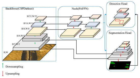
Figure 1.
The architecture of YOLO-C.
3.1. Backbone Network of YOLO-C
YOLO-C uses CSPDarknet53 with Focus as the backbone network to obtain features from input SSS imagery after data augmentation. The primary motivation is that CSPDarknet53 [23] has a relatively small number of parameters and a lower computation cost. It solves the problem of gradient duplication during optimization [33]. Therefore, it is conducive to ensuring the real-time performance of the network, which makes it suitable for feature extraction from input imagery in the context of YOLOv4, YOLOv5, and YOLOX [23,24,25].
Compared to previous seabed sediment recognition work based on side-scan sonar (SSS), the key difference in using YOLO-C is its ability to take the entire image as input and perform real-time recognition. It eliminates the need for feature selection methods to reduce feature dimensions. The convolutional neural network (CNN) incorporated in YOLO-C can extract more features, compensating for the potential lack of certain beneficial features in manually selected feature sets, especially in complex sediment environments.
The Focus module is a down-sampling method used in the backbone network that compresses the feature map while retaining model information. It reduces the spatial dimension of the feature map from (B, C, H, W) to (B, C*4, H/2, W/2) without any parameters and has a faster computation speed than traditional convolutional structures. To apply this method to input imagery, the spatial dimensions of the imagery are compressed using the Focus structure, and the compressed imagery is stacked according to channels dimension. The module with Focus can achieve faster inference speed while preserving most of the original information. Therefore, the Focus module provides a more efficient and effective alternative for feature extraction and representation learning in deep neural networks. Figure 2 illustrates the visual effects of this compression, which yields four pieces of compressed imagery.
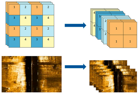
Figure 2.
The process of the Focus for the input imagery.
3.2. Feature Fusion of YOLO-C
Due to the complex variations in the shapes of objects in seabed sediment, the limited representation capacity of single-layer convolutional neural networks poses significant challenges in effectively representing and processing multi-scale features. To address the demand of multi-scale features, the bottom-up feature fusion operation of PANet [33] based on a feature pyramid network (FPN) is introduced. It can be understood that the role of FPN is to propagate high-level semantic information from the top feature to the bottom feature. In contrast, the role of the Bottom-up is to propagate low-level detailed information from the bottom feature to the top feature. It can efficiently facilitate the fusion of detailed and semantic features between different scales to improve object detection accuracy. However, interpreting and identifying the multi-scale seabed sediments in SSS imagery is often challenging due to their complex and heterogeneous nature. To improve the feature fusion capabilities and predictive robustness of YOLO-C, we introduce a new fusion structure on top of PAFPN [34], which enhances the integration of low-level and high-level information, as shown in Figure 3.
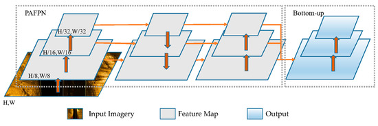
Figure 3.
Feature Fusion of YOLO-C.
3.3. Detect Head of YOLO-C
The YOLO-C model adopts the decoupled head [25] used in YOLOX. The decoupled head decomposes the detection head into a classification sub-head and a regression sub-head, which enables more flexible handling of object detection tasks and improves detection accuracy. Furthermore, the classification and regression sub-headers can be processed in parallel, which offers the potential to increase the detection speed of YOLO-C over traditional object detection algorithms. Additionally, its decoupled head can be adjusted according to different object detection tasks, making it more adaptable to various scenarios and applications. By dividing the detection head into classification and regression sub-heads, the object-detection problem can be separated into two sub-problems that are easier to optimize and debug. This approach also provides better interpretability and performance analysis.
A decoupled head used in YOLO-C can alleviate the conflict between the regression and classification tasks and reduce the number of parameters with faster inference speed. In YOLO-C, the spatial resolutions of the three detection heads are H/32, W/32, H/16, W/16, and H/8, W/8 for large-scale, medium-scale, and small-scale samples, respectively. At each layer of FPN features, we utilize a 1 × 1 convolutional layer to reduce the number of feature channels to 256. Then, we incorporate two separate branches for classification (cls.) and regression (reg.) tasks, each comprising two parallel 3 × 3 convolutional layers. A confidence score (conf.) branch is additionally included in the regression branch. The detection head is shown in Figure 4.
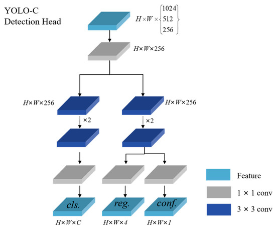
Figure 4.
The detect head of YOLO-C.
3.4. Segment Head of YOLO-C
The segment function of YOLO-C is mainly based on an encoder–decoder, like FCN and U-Net, etc. It is worth noting that the three-stage features used at the top of the decoder are the result of feature fusion.
The specific encoder–decoder structure in YOLO-C is shown in Figure 5, where a similar structure to the encoder (backbone) network is maintained in the decoder. It is worth noting that the encoder uses the convolution of stride 2 to down-sample the feature map, while the decoder uses the transposed convolution of dilation 2 to up-sample the feature map. On the one hand, feature fusion can efficiently enhance the multi-scale information of the model, and the information after feature fusion used in the detection branch largely promotes the segmentation performance without increasing the computational complexity of the segmentation branch. On the other hand, the YOLO-C model achieves an efficient fusion of segmentation and detection results while maintaining the same feature fusion information as the detection branch, which to some extent, avoids the problem of misalignment of upstream information.
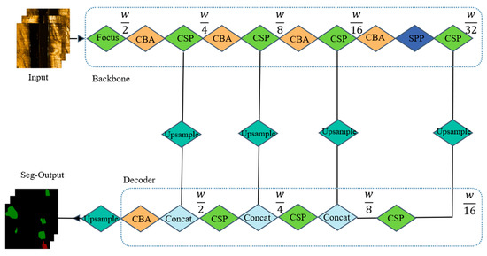
Figure 5.
Segment head of YOLO-C.
The proposed approach aims to efficiently fuse the results of semantic segmentation and object detection to enhance the object-contextual representations of the segmentation branch and the multi-scale information of the detection branch. To achieve this, the Softmax function is utilized to calculate the feature representation based on the output of the segmentation branch, denoted as “Featureseg”, shown in Formula (1). The resulting feature representation is then subject to down-sampling through a max-pooling layer. Featureseg1, Featureseg2, and Featureseg3 with the same spatial scale as the three detection heads are obtained by down-sampling Featureseg with max-pool, respectively. The confidence of the foreground is obtained according to Featuresegi, and the product of the foreground confidence and the confidence in Featuredet-conf. Featuredeti is performed according to the spatial dimension, as shown in Formula (2). Similarly, the classification scores of sand wave and rock are obtained according to Featuresegi using the Softmax function, and then the production operation is performed with the category features in Featuredet-cls according to the spatial dimension, as shown in Formula (3). These techniques enable effective fusion of the results of semantic segmentation and object detection, leading to improved object detection performance.
The loss function of the YOLO-C model consists of detection loss and segment loss. The loss in the detection branch (Ldet) mainly includes regression (location) loss and classification (category and confidence) loss. The location loss (Llocation) in the detection branch is obtained by intersection over union (IoU), shown in Formulas (4) and (5).
where A is the ground truth, and B is the predicted result.
The confidence loss (Lconfidence) in the detection branch is calculated by the binary cross entropy loss (LBCE), shown in Formula (6).
where xi represents the ground truth, and yi represents the predicted result after calculation using the Sigmoid function.
In the segmentation task (LSeg), no auxiliary loss or class balance loss, such as focal loss, is introduced. instead, a simple cross entropy (LCE) is used to achieve the final per-pixel classification task (LCEseg), as shown in Formula (7). To maintain the association with the semantic segmentation model, LCE is also used to calculate the category loss in the detection branch (LCEdet).
where C represents the number of classes, xi represents the ground truth label, and yi represents the prediction result after using Softmax. The total loss (Lall) of the model is shown in formula (8).
4. Experimental Results and Analysis
In this section, we introduce the datasets and evaluation metrics used in our experiments. Additionally, detailed evaluation results in both quantitative and qualitative are presented.
4.1. Experimental Dataset
4.1.1. TWS Seabed Dataset
The experimental data were gained by the Klein 3000 SSS system, which uses dual-frequency sonar (100 kHz and 500 kHz) to detect 100 m on each side while maintaining a high resolution of objects at a closer range. The data were collected from the Taiwan Strait between 2012 and 2022. The water depth of the surveyed area is about 10–35 m. The original side-scan data were analyzed using SonarPro software. In this paper, 207 pieces of imagery of seabed sediment containing sand waves, rocks, and sandy silt with a size of 1280 × 720 pixels were selected, called TWS Seabed Dataset. Some sediment examples are shown in Figure 6. To label the side scan imagery, we utilized two popular image-labeling software tools. Labelme [35] is for segmentation. LabelImg [36] is for object detection. For segmentation, Labelme saves the pixel information and the category information of the labeled polygonal objects in a JSON file in sequential order for each piece of imagery. On the other hand, for object detection, LabelImg saves the image’s resolution, the pixel coordinates of the borders’ upper-left and lower-right corners, and the category information of the borders in a TXT file. In total, 216 rocks and 125 sand waves are labeled. Examples of the manually labeled imagery by Labelme and LabelImg are shown in Figure 7a,b, respectively.
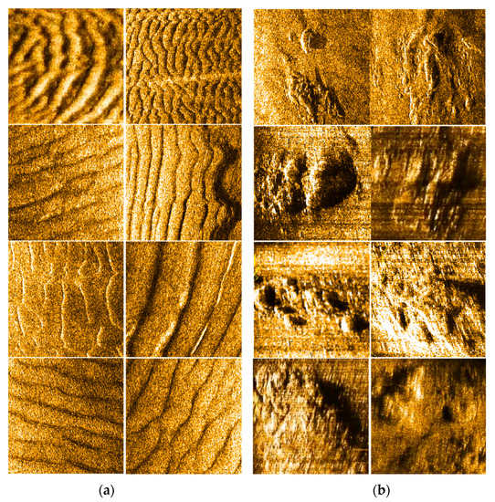
Figure 6.
Some sediment examples of (a) sand waves and (b) rock.
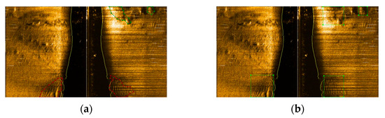
Figure 7.
The examples of label results. (a) The label of segmentation, and (b) the label of objection.
Due to the scarcity of datasets in side-scan sonar, we utilize practical data augmentation techniques, such as mosaic and the incorporation of random-vertical-flip [37], to enhance the dataset; the effectiveness of the data augmentation method is demonstrated in Figure 8a,b. To evaluate the feasibility and effectiveness of the new model YOLO-C, the publicly available xBD dataset [35] is also used for training and testing.
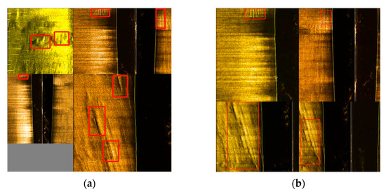
Figure 8.
Examples of data augmentation results. (a) Mosaic and (b) random-vertical-flip.
4.1.2. xBD Dataset
To validate the effectiveness of our proposed model, we conducted additional experiments using the xBD dataset [38]. The xBD dataset serves as an important benchmark for assessing building damage caused by various natural disasters, and its diverse and comprehensive collection of high-resolution satellite imagery enables a thorough evaluation of our model’s performance in real-world disaster scenarios. The xBD dataset comprises a substantial collection of 850,736 annotated buildings, covering an extensive area of 45,362 square kilometers in high-resolution satellite imagery.
This study focuses on verifying the applicability of the proposed YOLO-C model to open-source datasets and demonstrating its ability to localize multi-scale targets in complex background images; therefore, the images of xBD from two time periods were combined to obtain the training set, validation set, and test set data used for segmentation, localization, and classification in the later stage. Furthermore, the dataset’s large scale, high spatial resolution, and diverse building types enabled us to thoroughly evaluate our model’s performance under various challenging scenarios. Figure 9 shows an example of the xBD dataset.
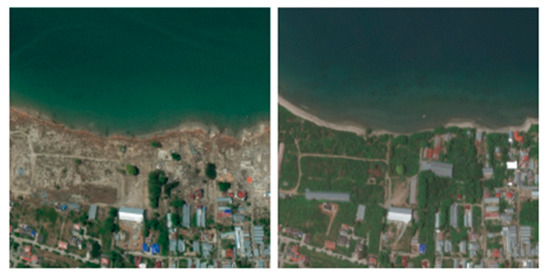
Figure 9.
Examples of the xBD dataset.
The results of our experiments on the xBD dataset reaffirmed the robustness and efficiency of our proposed model in accurately detecting building damage and identifying affected areas. The model’s superior performance on this challenging dataset further validates its effectiveness and demonstrates its potential for practical applications in disaster response and recovery efforts. Figure 9 shows the example of the xBD dataset.
4.2. Experimental Setup
The experimental environment: Python 3.7, Pytorch 1.71, Cuda 11.1, CPU is 11th Gen Intel(R) Core(TM) i7-11800H, and GPU is NVIDIA GeForce RTX 3060. The training process consists of two steps, with a total of 100 epochs. In the first step, the batch size is set to 16, the initial learning rate is 0.0001, and the learning rate is updated per epoch with a decay rate of 0.92. In the second step, the batch size is set to 8, the initial learning rate is 0.00001, and the learning rate per training epoch is updated with a decay rate of 0.92. Table 1 provides a detailed overview of the hyperparameters, including input size, activation function, optimizer, loss function, and other relevant parameters.

Table 1.
Main hyperparameters used for training and testing of YOLO-C.
4.3. Evaluation Metrics
In order to evaluate the effectiveness of seabed sediment detection from a comprehensive perspective, this paper adopts mPA (mean pixel accuracy), mIoU (mean intersection over union), MAE (mean absolute error), precision, and recall as the main evaluation indicators. mIoU calculates the precision rate of each pixel of the output result category by category.
Precision refers to the proportion of correctly predicted instances of a certain class out of the total predicted instances of that class, as shown in Formula (9). Recall refers to the proportion of correctly predicted instances of a certain class out of the total actual instances of that class, as shown in Formula (10). TP refers to true positives, FP refers to false positives, and FN refers to false negatives.
mAP is used to measure the average accuracy of predictions for each category. Precision@r is the precision when recall is r, where R is the selected number of recalls and n is the number of categories in object detection (especially in seabed sediments detection, n = 2), as shown in Formula (11).
PA is a metric that can be utilized to assess the accuracy of pixel-level predictions by calculating the proportion of correctly predicted pixels out of the total number of pixels. It is represented by Formula (12), which denotes the number of objects predicted as category j that truly belong to category i. Here, n represents the total number of categories.
mPA is utilized to assess the average ratio of accurately predicted pixels for each class, as shown in Formula (13).
mIoU is a classic evaluation metric for semantic segmentation, which is calculated by Formula (14), where n represents the number of categories and can be understood as the number of pixels where class i is predicted as class j.
MAE serves as a reliable evaluation metric to measure the average absolute difference between predicted values (ŷ) and actual values (y), as shown in the Formula (15), in which n is the number of output or Label image pixels
4.4. Results and Discussion
The presented study compared the performance of the YOLOX, U-Net, DeepLabv3+ [39], Segformer [40], PSPNet, YOLOv5, YOLOv7, YOLOv8, and our proposed YOLO-C model, which integrates the strengths of object detection and segmentation. The recognition results are presented in Figure 8, where (Figure 10a) represents the input imagery sample, (Figure 10b) depicts the ground truth, (Figure 10c) showcases the output of U-Net, (Figure 10d) demonstrates the results of DeepLabv3+, (Figure 10e) illustrates the effect of Segformer, (Figure 10f) displays the output of PSPNet, (Figure 10g) presents YOLOX, (Figure 10h) shows YOLOv5, (Figure 10i) represents YOLOv7, (Figure 10j) displays YOLOv8, and (Figure 10k) demonstrates the output of YOLO-C. It is worth noting that in the PSPNet model, some images were not detected, and similarly, YOLOv5, YOLOv7, and YOLOv8 models also exhibited partially undetected images. However, the proposed YOLO-C model showed improved performance in detecting and segmenting the objects of interest, as evident from the results depicted in Figure 10.
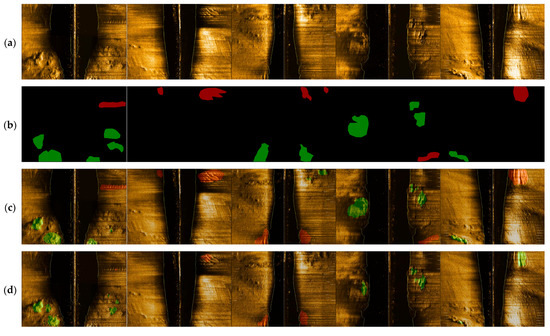
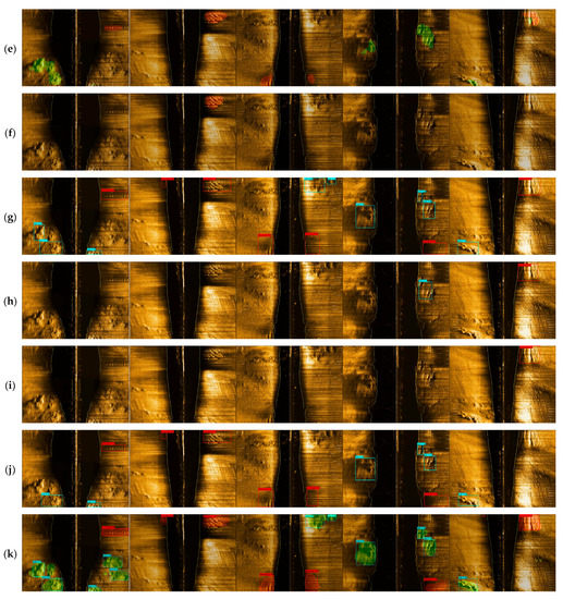
Figure 10.
The comparison of the TWS seabed dataset recognition results. (a) Original imagery, (b) the ground truth, (c) the effect of U-Net, (d) the effect of DeepLabv3+, (e) the performance of segformer, (f) the effect of PSPNet, (g) the performance of YOLOX, (h) the effect of YOLOv5, (i) the performance of YOLOv7, (j) the effect of YOLOv8, and (k) the performance of YOLO-C.
Among the results in the semantic segmentation and object detection tasks, they can be classified as TP, FP, true negative (TN), and FN. The confusion matrix is a unique contingency table with two dimensions (actual and predicted) and the same categories in both dimensions. In the case of multi-class classification, the confusion matrix represents the number of times the model predicts one class as another class. The cells on the main diagonal of the matrix indicate the number of correct predictions made by the model, while the off-diagonal cells represent the number of misclassifications. It can be inferred from Table 2 that the model has good discrimination between sand waves and rocks.
Table 2.
Confusion matrix of YOLO-C.
In object detection, AP is a standard metric that measures the precision of the model. The results demonstrate the superiority of YOLO-C in object detection compared to the reference model YOLOX. The AP value of YOLO-C is generally higher than that of YOLO, which is further confirmed by the comparison of their mAP values. The comparison of AP values between YOLOX, YOLOv5, YOLOv7, YOLOv8, and YOLO-C in Figure 11 shows that YOLO-C outperforms YOLO. The improvement in performance is also evident in the mAP comparison in Table 3, which describes the metrics of different methods to detect the segmentation and detection of sonar imagery of seabed sediments.
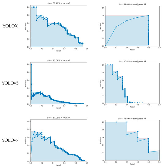
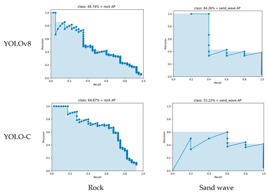
Figure 11.
The comparison of YOLOX, YOLOv5, YOLOv7, YOLOv8, and YOLO-C about AP values.
Table 3.
The comparison of the indicators of each method.
The performance of our proposed YOLO-C model was compared to several state-of-the-art models, including YOLOX, YOLOv5, YOLOv7, YOLOv8, DeepLabv3+, Segformer, PSPNet, and U-Net. The comparison results, as shown in Table 3, highlight the superior performance of YOLO-C in detecting and classifying seabed sediments. YOLO-C achieved the highest mean average precision (mAP) of 58.94%, surpassing YOLOX (mAP: 57.64%), YOLOv5 (mAP: 21.74%), YOLOv7 (mAP: 55.47%), and YOLOv8 (mAP: 57.0%).
In terms of semantic segmentation, YOLO-C also outperformed the newly introduced models. It achieved a higher mean intersection over union (mIoU) compared to DeepLabv3+ (mIoU: 56.03%), Segformer (mIoU: 67.41%), and PSPNet (mIoU: 50.85%). Similarly, YOLO-C exhibited higher mean pixel accuracy (mPA) than DeepLabv3+ (mPA: 71.38%), Segformer (mPA: 74.59%), and PSPNet (mPA: 56.93%). Furthermore, YOLO-C demonstrated a lower MAE of 0.0345, indicating better segmentation accuracy than DeepLabv3+ (MAE: 0.0437), Segformer (MAE: 0.0564), and PSPNet (MAE: 0.0544).
The outstanding performance of YOLO-C can be attributed to its unique fusion of object detection and semantic segmentation techniques. The integration of these approaches enables precise identification, accurate boundary detection, and detailed segmentation of seabed sediments. The comprehensive recognition of sediment features contributes to the improved accuracy and performance of YOLO-C when compared to other state-of-the-art models.
In summary, the comparison and analysis of mAP, mIoU, mPA, and MAE metrics demonstrate the exceptional performance of our proposed YOLO-C model in detecting, classifying, and segmenting seabed sediments. YOLO-C outperforms the benchmark models, including the newly introduced DeepLabv3+, Segformer, PSPNet, and various YOLO variants (YOLOX, YOLOv5, YOLOv7, and YOLOv8), highlighting its superiority in terms of accuracy and performance in the field of seabed sediment analysis.
We also calculate the area of the seabed sediment to be detected for each algorithm. Table 4 shows the area of YOLOX, U-Net, Mask R-CNN [33], and YOLO-C for the imagery in the TWS seabed dataset (15.jpg is a sample detection result). YOLO-C can more accurately represent the shape and position of objects, provide more detailed object information, and thus enable more accurate calculations of object areas compared to bounding boxes.
Table 4.
The area of different models.
To demonstrate the efficient integration of the semantic segmentation branch and detection branch in YOLO-C, this paper employs the Grad-CAM algorithm [34] to visualize the feature information of the fused detection branch, as shown in Figure 12. Here, (Figure 12a) represents the original imagery, (Figure 12b) represents the detection result of YOLO-C, (Figure 12c) represents the visualization heat map of YOLOX, (Figure 12d) is the visualization heat map of YOLOv5, (Figure 12e) represents the visualization heat map of YOLOv7, (Figure 12f) is the visualization heat map of YOLOv8, and (Figure 12g) represents the visualization heat map of YOLO-C. It can be observed that the information extracted by YOLO-C can accurately perceive seabed sediment. Therefore, YOLO-C is of high practical value. It can clearly demonstrate the neural network’s response level to a specific region. The visualization results provided by the Grad-CAM algorithm support the effectiveness of YOLO-C in accurately identifying seabed sediments. The heat maps generated by YOLO-C demonstrate its ability to capture and localize the relevant features related to the target objects. In comparison to YOLOX, YOLO-C exhibits superior performance in terms of precise target detection, as indicated by the more focused and concentrated heat map patterns. Furthermore, the integration of the semantic segmentation branch and detection branch in YOLO-C facilitates a synergistic combination of their strengths. The semantic segmentation branch contributes rich contextual information and precise boundary localization, while the detection branch enhances the model’s recognition capability for multi-scale targets. This complementary relationship between the two branches leads to improved performance in terms of both accuracy and efficiency.
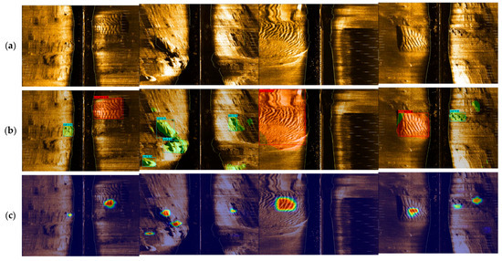
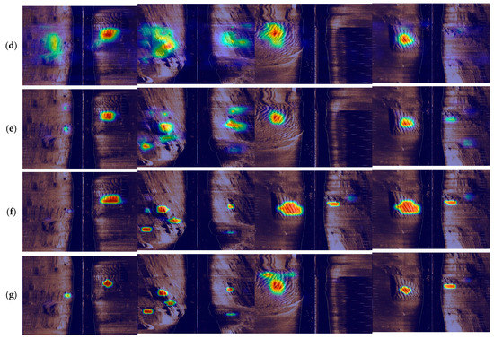
Figure 12.
The feature information of the fused detection branch by Grad-CAM. (a) Original imagery, (b) the detection result of YOLO-C, (c) the visualization heat map of YOLOX., (d) the visualization heat map of YOLOv5, (e) the visualization heat map of YOLOv7, (f) the visualization heat map of YOLOv8, and (g) the visualization heat map of YOLO-C.
The utilization of the Grad-CAM visualization technique not only enhances our understanding of the inner workings of YOLO-C but also validates its effectiveness in capturing relevant features for seabed sediment recognition. By visually analyzing the heat maps, we can observe the neural network’s focus on specific regions of interest and confirm the model’s ability to accurately identify and distinguish seabed sediment targets.
To verify the universality of the YOLO-C model, we conduct experiments on another public dataset, xBD, of remote sensing image-based building hazards. Firstly, we divide the classes into background and building. Secondly, we obtain the detection box information from the label of semantic segmentation, which can achieve two tasks in semantic segmentation and object detection. The 1280 × 1280 resolution image is used as the input image for processing. Figure 13 shows the comparison results of different models. The comparison results depicted in Figure 13 affirm the efficacy of our proposed model, YOLO-C, across multiple datasets. Its superior performance in both seabed sediment analysis and building damage assessment showcases its versatility, reliability, and generalizability. These findings emphasize the broad potential of YOLO-C for a range of applications and further support its adoption in scientific research and real-world scenarios.
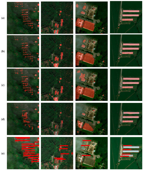
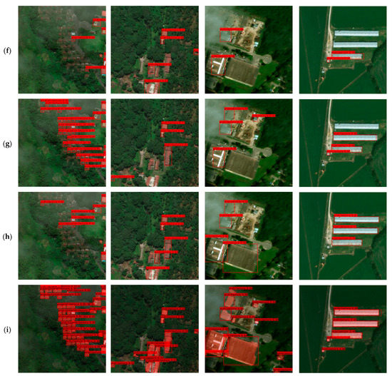
Figure 13.
The comparison of the xBD Dataset recognition results. (a) The effect of U-Net, (b) the effect of DeepLabv3+, (c) the performance of segformer, (d) the effect of PSPNet, (e) the performance of YOLOX, (f) the effect of YOLOv5, (g) the performance of YOLOv7, (h) the effect of YOLOv8, and (i) the performance of YOLO-C.
To compare the performance between YOLO-C and traditional models, Table 5 presents the different evaluation metrics for these two datasets. The results showed that YOLO-C achieved better performance than traditional models in terms of both efficiency and accuracy, which can be quantified by the metric FPS, mAP, mIoU, and so on.
Table 5.
Performance comparison of different algorithms.
Based on the comprehensive performance evaluation conducted in this study, our proposed YOLO-C algorithm has demonstrated superior performance compared to state-of-the-art models in the field of seabed sediment detection and segmentation. By leveraging the full-resolution classification feature of its semantic segmentation algorithm and incorporating the target region localization ability of the target detection algorithm, YOLO-C exhibits exceptional recognition capabilities for multi-scale targets.
The evaluation results on the TWS seabed, and xBD datasets consistently highlight the effectiveness of YOLO-C. It achieves a higher mean average precision (mAP) of 58.94%, F1 score of 41.50, mean intersection over union (mIoU) of 70.36%, and mean pixel accuracy (mPA) of 91.80% compared to the reference models. Additionally, YOLO-C demonstrates significantly faster frame-per-second (FPS) rates, with a segmentation speed of 198 fps and a combined segmentation and detection speed of 98 fps. These results confirm that YOLO-C not only meets the real-time detection requirements for seabed sediment targets but also maintains high efficiency in practical applications.
Furthermore, the performance comparison against prominent models, including YOLOX, YOLOv5, YOLOv7, YOLOv8, U-Net, DeepLabv3+, Segformer, and PSPNet, consistently showcases the superiority of YOLO-C in terms of mAP, F1 score, mIoU, and mPA values. This indicates that YOLO-C excels in accurately detecting, classifying, and segmenting seabed sediments, surpassing existing methods.
Moreover, the efficiency of YOLO-C is a key advantage, as it achieves remarkable accuracy without compromising time efficiency. This capability enables real-time or near-real-time seabed sediment recognition, which is critical for time-sensitive tasks such as marine resource exploration, environmental monitoring, and underwater surveys.
In conclusion, our proposed YOLO-C algorithm has demonstrated exceptional performance and efficiency in the detection, classification, and segmentation of seabed sediments. The integration of the full-resolution classification feature and target region localization ability enhances its recognition capabilities and surpasses existing models. The superior performance and efficiency of YOLO-C make it a valuable tool for a wide range of applications in marine research, resource assessment, environmental monitoring, and underwater archaeology.
5. Conclusions
The paper proposes a novel segmentation model YOLO-C, which combines the advantages of U-Net and YOLOX. Our model achieves higher accuracy and produces more precise segmentation with fast speed. This proposed method enhances the detection capability by incorporating masks, which facilitate more accurate area calculations of the objects compared to the well-known Mask R-CNN algorithm. We evaluate the proposed method on the TWS seabed dataset and xBD, and the results show its better performance on mAP, mIoU, and mPA compared to other methods. Additionally, YOLO-C outperforms both detection and segmentation methods in terms of processing speed, exhibiting a segmentation speed that is 188 frames per second faster. The overall speed, inclusive of both segmentation and detection, is 98 fps, which demonstrates its real-time detection capability.
Future work aims to focus on enhancing the detection performance of small objects in SSS imagery. This would enable further testing and enhancement of the system in this domain and could have practical significance for extending the model to side-scan sonar automatic recognition.
Author Contributions
Conceptualization, X.C. and P.S.; methodology, X.C.; software, X.C.; validation, Y.H., P.S. and X.C.; formal analysis, P.S.; investigation, Y.H.; resources, Y.H.; data curation, X.C.; writing—original draft preparation, X.C.; writing—review and editing, P.S.; visualization, X.C.; supervision, P.S.; project administration, P.S. All authors have read and agreed to the published version of the manuscript.
Funding
This work was funded by the Fujian Science and Technology Program Guiding Project (2022Y0070) and the Xiamen Ocean Research and Development Institute Project “Development of Multi-unit Marine Single Channel Seismic Solid Cable”.
Institutional Review Board Statement
Not applicable.
Informed Consent Statement
Not applicable.
Data Availability Statement
Not applicable.
Conflicts of Interest
The authors declare no conflict of interest.
References
- Tęgowski, J. Acoustical classification of the bottom sediments in the southern Baltic Sea. Quat. Int. 2005, 130, 153–161. [Google Scholar] [CrossRef]
- Lamarche, L.G. Unsupervised fuzzy classification and object-based image analysis of multibeam data to map deep water substrates, Cook Strait, New Zealand. Cont. Shelf Res. 2011, 31, 1236–1247. [Google Scholar]
- Lucieer, V.; Lucieer, A. Fuzzy clustering for seafloor classification. Mar. Geol. 2009, 264, 230–241. [Google Scholar] [CrossRef]
- Lark, R.M.; Dove, D.; Green, S.L.; Richardson, A.E.; Stewart, H.; Stevenson, A. Spatial prediction of seabed sediment texture classes by cokriging from a legacy database of pointobservations. Sediment. Geol. 2012, 281, 35–49. [Google Scholar] [CrossRef]
- Huvenne, V.A.I.; Blondel, P.; Henriet, J.P. Textural analyses of sidescan sonar imagery from two mound provinces in the Porcupine Seabight. Mar. Geol. 2002, 189, 323–341. [Google Scholar] [CrossRef]
- Haralick, R.M. Textural features for image classification. IEEE Trans. Syst. Man Cybern. 1973, 6, 610–621. [Google Scholar] [CrossRef]
- Li, J.; Heap, A.D.; Potter, A.; Huang, Z.; Daniell, J.J. Can we improve the spatial predictions of seabed sediments? A case study of spatial interpolation of mud content across the southwest Australian margin. Cont. Shelf Res. 2011, 31, 1365–1376. [Google Scholar] [CrossRef]
- Cui, X.; Yang, F.; Wu, Z.; Zhang, K.; Ai, B. Deep-sea sediment mixed pixel decomposition based on multibeam backscatter intensity segmentation. IEEE Trans. Geosci. Remote Sens. 2021, 99, 1–15. [Google Scholar] [CrossRef]
- Marsh, I.; Brown, C. Neural network classification of multibeam backscatter and bathymetry data from Stanton Bank (Area IV). Appl. Acoust. 2009, 70, 1269–1276. [Google Scholar] [CrossRef]
- Berthold, T.; Leichter, A.; Rosenhahn, B.; Berkhahn, V.; Valerius, J. Seabed sediment classification of side-scan sonar data using convolutional neural networks. In Proceedings of the 2017 IEEE Symposium Series on Computational Intelligence (SSCI), Honolulu, HI, USA, 27 November–1 December 2017; IEEE: Piscataway, NJ, USA; pp. 1–8. [Google Scholar] [CrossRef]
- Xi, H.Y.; Wan, L.; Sheng, M.W.; Li, Y.M.; Liu, T. The study of the seabed side-scan acoustic images recognition using BP neural network. In Parallel Architecture, Algorithm and Programming; Springer: Singapore, 2017; pp. 130–141. [Google Scholar]
- Sun, C.; Hu, Y.; Shi, P. Probabilistic neural network based seabed sediment recognition method for side-scan sonar imagery. Sediment. Geol. 2020, 410, 105792. [Google Scholar] [CrossRef]
- Steele, S.M.; Ejdrygiewicz, J.; Dillon, J. Automated synthetic aperture sonar image segmentation using spatially coherent clustering. In Proceedings of the OCEANS 2021: San Diego—Porto, San Diego, CA, USA, 20–23 September 2021; Volume 3, p. 16. [Google Scholar]
- Qin, X.; Luo, X.; Wu, Z.; Shang, J. Optimizing the sediment classification of small side-scan sonar images based on deep learning. IEEE Access 2021, 9, 29416–29428. [Google Scholar] [CrossRef]
- Zheng, G.; Zhang, H.; Li, Y.; Zhao, J. A universal automatic bottom tracking method of side scan sonar data based on semantic segmentation. Remote Sens. 2021, 13, 1945. [Google Scholar] [CrossRef]
- Chen, J.; Zhang, S. Segmentation of sonar image on seafloor sediments based on multiclass SVM. J. Coast. Res. 2018, 83, 597–602. [Google Scholar] [CrossRef]
- Viola, P.A.; Jones, M.J. Rapid object detection using a boosted cascade of simple features. In Proceedings of the 2001 IEEE Computer Society Conference on Computer Vision and Pattern Recognition. CVPR 2001, Kauai, HI, USA, 8–14 December 2001; IEEE: Piscataway, NJ, USA; pp. 511–518. [Google Scholar] [CrossRef]
- Dalal, N.; Triggs, B. Histograms of Oriented Gradients for Human Detection. In Proceedings of the 2005 IEEE Computer Society Conference on Computer Vision and Pattern Recognition, San Diego, CA, USA, 20–25 June 2005; IEEE: Piscataway, NJ, USA; pp. 886–893. [Google Scholar]
- Felzenszwalb, P.F.; Girshick, R.B.; McAllester, D.; Ramanan, D. Object detection with discriminatively trained part-based models. IEEE Trans. Pattern Anal. Mach. Intell. 2009, 32, 1627–1645. [Google Scholar] [CrossRef] [PubMed]
- Redmon, J.; Divvala, S.; Girshick, R.; Farhadi, A. You only look once: Unified, real-time object detection. In Proceedings of the IEEE Conference on Computer Vision and Pattern Recognition, Las Vegas, NV, USA, 27–30 June 2016; pp. 779–788. [Google Scholar]
- Redmon, J.; Farhadi, A. YOLO9000: Better, Faster, Stronger. In Proceedings of the IEEE Conference on Computer Vision and Pattern Recognition, Honolulu, HI, USA, 21–26 July 2017; pp. 6517–6525. [Google Scholar]
- Redmon, J.; Farhadi, A. Yolov3: An incremental improvement. arXiv 2018, arXiv:1804.02767. [Google Scholar]
- Bochkovskiy, A.; Wang, C.Y.; Liao, Y.H.M. Yolov4: Optimal speed and accuracy of object detection. arXiv 2020, arXiv:2004.10934. [Google Scholar]
- Ultralytics. YOLOv5. 2020. Available online: https://github.com/ultralytics/YOLOv5 (accessed on 3 March 2022).
- Ge, Z.; Liu, S.; Wang, F.; Li, Z.; Sun, J. Yolox: Exceeding yolo series in 2021. arXiv 2021, arXiv:2107.08430. [Google Scholar]
- Li, C.; Li, L.; Jiang, H.; Weng, K.; Geng, Y.; Li, L.; Wei, X. YOLOv6: A single-stage object detection framework for industrial applications. arXiv 2022, arXiv:2209.02976. [Google Scholar]
- Wang, C.Y.; Bochkovskiy, A.; Liao, Y.H.M. YOLOv7: Trainable bag-of-freebies sets new state-of-the-art for real-time object detectors. In Proceedings of the IEEE/CVF Conference on Computer Vision and Pattern Recognition, Vancouver, BC, Canada, 18–22 June 2023; pp. 7464–7475. [Google Scholar]
- Ren, S.; He, K.; Girshick, R.; Sun, J. Faster R-CNN: Towards real-time object detection with region proposal networks. IEEE Trans. Pattern Anal. Mach. Intell. 2017, 39, 1137–1149. [Google Scholar] [CrossRef]
- Long, J.; Shelhamer, E.; Darrell, T. Fully convolutional networks for semantic segmentation. IEEE Trans. Pattern Anal. Mach. Intell. 2015, 39, 640–651. [Google Scholar]
- Ronneberger, O.; Fischer, P.; Brox, T. U-Net: Convolutional networks for biomedical image segmentation. In International Conference on Medical Image Computing and Computer-Assisted Intervention; Springer: Cham, Switzerland, 2015; pp. 234–241. [Google Scholar]
- Chen, L.C.; Papandreou, G.; Kokkinos, I.; Murphy, K.; Yuille, A.L. Deeplab: Semantic image segmentation with deep convolutional nets, atrous convolution, and fully connected crfs. IEEE Trans. Pattern Anal. Mach. Intell. 2018, 40, 834–848. [Google Scholar] [PubMed]
- Zhao, H.; Shi, J.; Qi, X.; Wang, X.; Jia, J. Pyramid scene parsing network. In Proceedings of the IEEE Conference on Computer Vision and Pattern Recognition, Honolulu, HI, USA, 21–26 July 2017; pp. 2881–2890. [Google Scholar]
- Liu, S.; Qi, L.; Qin, H.; Shi, J.; Jia, J. Path aggregation network for instance segmentation. In Proceedings of the IEEE Conference on Computer Vision and Pattern Recognition, Salt Lake City, UT, USA, 18–23 June 2018; pp. 8759–8768. [Google Scholar]
- Li, Z.; Zhou, F. FSSD: Feature fusion single shot multibox detector. arXiv 2017, arXiv:1712.00960. [Google Scholar]
- Wkentaro. LabelMe. 2010. Available online: https://github.com/wkentaro/labelme (accessed on 10 September 2021).
- HeartaxLab. LabelImg. Available online: https://github.com/heartexlabs/labelImg (accessed on 14 September 2021).
- WesMcKinney. Transform. 2020. Available online: https://pytorch.org/vision/main/generated/torchvision.transforms.RandomVerticalFlip.html (accessed on 1 July 2022).
- Gupta, R.; Goodman, B.; Patel, N.; Hosfelt, R.; Sajeev, S.; Heim, E.; Doshi, J.; Lucas, K.; Choset, H.; Gaston, M. Creating xBD: A Dataset for Assessing Building Damage from Satellite Imagery. In Proceedings of the IEEE Conference on Computer Vision and Pattern Recognition Workshops, Long Beach, CA, USA, 16–20 June 2019; pp. 10–17. [Google Scholar]
- Chen, L.C.; Zhu, Y.; Papandreou, G.; Schroff, F.; Adam, H. Encoder-decoder with atrous separable convolution for semantic image segmentation. In Proceedings of the European Conference on Computer Vision (ECCV), Munich, Germany, 8–14 September 2018; Springer: Berlin/Heidelberg, Germany, 2018; pp. 801–818. [Google Scholar]
- Xie, E.; Wang, W.; Yu, Z.; Anandkumar, A.; Alvarez, J.M.; Luo, P. SegFormer: Simple and efficient design for semantic segmentation with transformers. Adv. Neural Inf. Process. Syst. 2021, 34, 12077–12090. [Google Scholar]


Disclaimer/Publisher’s Note: The statements, opinions and data contained in all publications are solely those of the individual author(s) and contributor(s) and not of MDPI and/or the editor(s). MDPI and/or the editor(s) disclaim responsibility for any injury to people or property resulting from any ideas, methods, instructions or products referred to in the content. |
© 2023 by the authors. Licensee MDPI, Basel, Switzerland. This article is an open access article distributed under the terms and conditions of the Creative Commons Attribution (CC BY) license (https://creativecommons.org/licenses/by/4.0/).