

Projected Sea Bottom Temperature Variability in the East China Shelf Seas by 2100
School of Marine Science and Technology, Tianjin University, Tianjin 300072, China
*
Author to whom correspondence should be addressed.
J. Mar. Sci. Eng. 2023, 11(6), 1192; https://doi.org/10.3390/jmse11061192
Submission received: 23 April 2023
/
Revised: 30 May 2023
/
Accepted: 2 June 2023
/
Published: 8 June 2023
(This article belongs to the Special Issue Estuaries, Coasts, and Seas in a Changing Climate)
Abstract
:Existing research has proven the increase in sea surface temperature (SST) due to global warming. However, the sea bottom temperature (SBT) may exhibit different characteristics in various regional seas. The East China Shelf Seas (ECSSs), which are important shelf seas in the Western Pacific, hold ecological significance when analyzing their SBT variations in a warming future. This article investigates both the interannual and interdecadal SBT variations from 2006 to 2100, utilizing the projection results from phase 5 of the Climate Model Intercomparison Project (CMIP5) sponsored by the Intergovernmental Panel on Climate Change (IPCC). We conducted an analysis of the interdecadal variation by comparing the SBTs from the 2030s, 2060s, and 2090s to the SBT observed in the 2010s. Our findings reveal a significant increase in SBT in the ECSSs. By 2100, the region is projected to experience enhanced warming of 1.18 °C. The springtime warming intensity of the Bohai Sea, reaching 1.92 °C, can be twice the rate of global ocean warming. The outer shelf of the ECSSs also exhibits significant increases in SBT. Through an analysis of the correlation between SBT and ocean currents, we investigate the potential mechanisms behind these observations. This paper provides insights into future SBT variations from both an interannual and interdecadal perspective, explaining the causes and the projected increase in environmental stresses on the benthic ecosystem over the next eighty years.
1. Introduction
The climate is undergoing changes, in which the greenhouse effect plays an important role [1,2]. Many believe that climate change could be one of the most serious threats to our world. Ocean warming has already become a significant problem, contributing significantly to global climate change. It has been accelerating and may persist over the next 100 years, according to the results of recent observation-based estimations and model simulations [3,4,5,6,7,8].
The East China Shelf Seas (ECSSs) are composed of the Bohai Sea, the Yellow Sea, and the East China Sea. They refer to the eastern marginal seas of China, which are surrounded by the Chinese mainland and the Korean Peninsula. Since the ECSSs are shallow, located at the eastern end of the largest continent in the world, and can respond quickly to climate change, they are recognized as some of the most important marginal seas in the Western North Pacific Ocean (WNPO) [9,10]. The ECSSs play important roles in the study of environmental and ecosystem issues due to their unique geographic locations and complex hydrography. The Bohai Sea is a semi-enclosed sea with an average depth of only 18 m. In comparison to the physical forcing from the open-ocean side, the temperature variation within its basin has a greater impact on its ecosystem [11,12]. The Yellow Sea, which covers a relatively larger area, is also quite shallow. The water depth over most of the Yellow Sea is less than 50 m. For this broad and shallow continental shelf sea, its water column is more susceptible to the atmospheric factors within itself than from the outer oceans [13]. The East China Sea is located between the world’s largest ocean and the largest continent. It is influenced by the climatic forcing from the Kuroshio Current in the tropic ocean and the East Asian Monsoon System in the high-latitude Northern Hemisphere. The combination of these two forces results in a distinct climate pattern of strong vertical and horizontal temperature gradients [14,15]. All of these marginal seas, which support heavy oil drilling, fishing, and shipping activities, hold significant social and economic importance for the people living in the coastal regions [16,17].
The response of the ECSSs to global warming is sensitive due to their shallow water depths [3]. The warming in this region, including the Japan Sea, is projected to increase by approximately 0.8 to 2 °C per century [18]. The metabolic rated of marine organisms and other oceanic conditions, such as local currents, are affected by the increase in sea temperature [19]. Thus, it is crucial to comprehend the spatial and temporal variabilities of the ECSSs, particularly in projecting the long-term variations in the future [3,19].
With the high development of ocean simulation technologies, climate change can be assessed through model intercomparison projects, among which, the coupled model intercomparison project plays a significant role [20,21]. The Intergovernmental Panel on Climate Change (IPCC) has sponsored phase 5 of the Climate Model Intercomparison Project (CMIP5), which provides a multimodal context for comprehending the responses of climate models to a common forcing. The goal is to facilitate climate model projection and evaluation for the Fifth Assessment Report (AR5) [21,22]. It comprises multiple models that can project future climate in a warming world under various representative concentration pathways (RCPs), such as RCP2.7, RCP4.5, RCP6.0, and RCP8.5. The RCPs will correspond to a top-of-the-atmosphere radiative imbalance of 2.6, 4.5, 6.0, and 8.5 W/m by 2100 [23]. CMIP5, which follows previous CMIPs, has emerged as a recently available experimental framework that addresses climate change projections for future scenarios, and can be used for interannual and interdecadal climate projections for global oceans.
In the literature, a large number of works have been developed to project climate changes using the simulation results of CMIP5. For example, Heuz et al. [24] studied the southern ocean’s deep water properties, including the southern ocean’s bottom density and temperatures from 1986 to 2005. Cheng and Zhu [23] proposed an advanced mapping method based on an ensemble optimal interpolation and a multimodal ensemble of CMIP5 historical simulations and RCP4.5 scenarios to reconstruct the historical temperature field of the ocean subsurface (0–700 m) from 1940 to 2014. Zhou and Ying [25] analyzed the Pacific interannual SST variability in the historical simulations and future analyses of RCP4.5 and RCP8.5. There have also been some results from studying climate changes using CMIP5 models in the Chinese coastal seas. Huang et al. [26] assessed the abilities of 17 CMIP5 models to simulate historical SSTs in the South China Sea (SCS). Based on this assessment, they also projected future SST changes in the 21st century under various RCPs. Huang and Qiao [27] estimated the future potential sea level changes in the SCS under different RCPs. Based on the simulated results of the CMIP5 models under RCP4.5, Tan et al. [28] assessed the SST trend for offshore China in the 21st century. Song et al. [29] used five representative CMIP5 models to analyze the monthly, seasonal, and interannual SSTs from 1960 to 2002 in the China Seas.
Existing works on the study of seawater temperature changes in the ECSSs mainly focus on the projection of SST changes, without investigating the changes in sea bottom temperature (SBT). The SBT, which is a key physical parameter of the benthic environment, plays a crucial role in adjusting the bottom biogeochemical and physical processes and controlling the growth and development of bottom organisms. Its spatial and temporal variations, which are usually coupled to climate changes, can greatly influence the structures and functions of bottom marine ecosystems [14,30]. SBT increases can intensify ecological problems in nearshore regions. For instance, due to the SBT increase, since 2009, there have been frequent brown tide breakouts in the coastal areas of Qinhuangdao in the Bohai Sea. Red and green tides, as well as jellyfish disasters, have recently affected the Changjiang Estuary and the shores in the northern Jiangsu province [11]. Thus, it is crucially important to project the long-term variations. Moreover, existing works have demonstrated that SSTs over worldwide oceans can increase due to global warming. However, the SBT may show different characteristics in different regional seas. The East China Shelf Seas are important marginal seas of the Western Pacific, characterized by relatively shallow water. It is much easier to be influenced by atmospheric changes. Thus, it is important to project and analyze SBT variations in future climate change scenarios.
Motivated by the aforementioned findings, we propose a CMIP5-based projection of SBT to analyze interannual and interdecadal variations in the ECSSs by 2100. The projection results of six representative models under RCP4.5 were used, i.e., ACCESS1.3, FIO-ESM, CCSM4, NorESM1-ME, CESM1-WACCM, and MPI-ESM-MR. We first calculated the SBT in the ECSSs according to the depth map of this region, which was used to determine the bottom layer. The model validation was performed using high-resolution hydrographic data from the World Ocean Atlas 2018 (WOA18) [31]. We utilized the most appropriate model, MPI-ESM-MR, which offers higher resolution and simulation accuracy compared to others, to analyze the interannual and interdecadal variability of SBT by 2100. RCP4.5 was used as a representative scenario because it provides a medium-mitigation emission scenario that stabilizes the direct radiative forcing at 4.5 W/m (650 ppm CO equivalent) [32,33]. When comparing RCP 4.5 to RCP8.5, it is evident that RCP8.5 results in significantly higher greenhouse gas emissions (at 8.5 W/m by 2100), while RCP2.6 leads to a very low forcing level (at 2.6 W/m by 2100). RCP4.5 is neither too low (as RCP2.6) nor too high (as RCP8.5) for projections. The essential ideas and most important findings of this paper are shown in Figure 1.
This paper is organized as follows: Section 2 introduces the data and method utilized for bottom temperature estimation. In Section 3, a model validation and simulation result modification strategy is presented using WOA18 data. The experimental results of interannual and interdecadal bottom temperature changes are analyzed in Section 4 and Section 5, respectively. This paper is concluded in Section 6.
2. Data and Method
2.1. Data
This paper utilizes CMIP5 model data from 2006 to 2100 for the analysis of future bottom temperature changes and introduces WOA18 data for the current analysis as well as for model validation. CMIP5 comprises 36 models provided by 16 institutes. In this paper, we utilize the most representative models based on two primary criteria: (1) for each institute, we only use the recently developed model with the highest resolution for our study; (2) the selected models provide continuous simulation results of seawater temperature along the depth, from 2006 to 2100, without any interruptions. Six representative models were selected in this paper: ACCESS1.3, FIO-ESM, CCSM4, NorESM1-ME, CESM1-WACCM, and MPI-ESM-MR. Table 1 shows the information on these models. From Table 1, it can be observed that MPI-ESM-MR has a significantly higher resolution compared to the other. MPI-ESM-MR is a general circulation model that couples the atmosphere and the ocean. It has been applied in numerous climate change studies involving idealized CO-only forcing, forcing based on RCP scenarios, and observations [34].
The WOA18 data from 2005 to 2017 were used to investigate the climatological annual mean and seasonal mean water temperature in 2010 for the current analysis and model validation. The WOA18 data provide objectively analyzed (1° grid) climatological fields of annual and seasonal seawater temperatures at standard depth levels of the World Ocean, providing associated statistical observation data interpolated to standard depth levels of 5°, 1°, and 0.25° grids [31]. We used a data grid with a resolution of 0.25° for the analysis.
The annual and seasonal mean water temperatures for 2010 were determined by the average results from 2006 to 2015 in order to reduce the inner simulation variations and errors in each CMIP5 model. Similar processing was applied to derive the average results for 2030, 2060, and 2090. The average results are 2026∼2035, 2056∼2064, 2086∼2094, respectively.
2.2. Study Area
The study area of this paper consists of the Bohai Sea, the Yellow Sea, and part of the East China Sea. The water depth map with contours of 0 m, 50 m, 100 m, 150 m, and 200 m, is shown in Figure 2. From Figure 2, we can see that the Bohai Sea is a semi-enclosed shallow sea with a water depth that is less than 50 m (the average depth is only 18 m). The East China Sea and the Yellow Sea cover relatively larger regions with water depths ranging from 50 to 200 m. Given the shallow water in these three seas, we calculated the annual and seasonal average vertical temperatures in 2010. Figure 3 shows the vertical temperature distribution in the Bohai Sea, Yellow Sea, and East China Sea. The horizontal axis indicates the temperature and the vertical axis indicates the water depth level.
2.3. Bottom Temperature Determination
This paper focuses on the projection of bottom temperature changes. However, neither the CMIP5 data nor the WOA18 data provide the bottom temperature value directly. Instead, they provide the simulation results of seawater temperature along the depth. To solve this problem, this paper calculates the bottom temperature according to the depth map of the study region. For each grid point, the bottom temperature can be determined by assigning the temperature at the sea bottom depth to it. The detailed procedure is as follows. For the depth (d) of a given grid point at the coordinates , we first calculate the vertical layer (, where z represents the number of vertical levels of each model in Table 1), where d is higher than the depth at layer k and lower than or equal to the depth of layer . Then, we assign the water temperature of layer k as the bottom temperature to this gird point. The same calculation goes for the other grid points. Finally, we can obtain the bottom temperature covering all of the grid points.
3. Model Validation and Simulation Result Improvement
Simulation results from numeric models are subject to some degree of error. Thus, model validation is necessary to evaluate the reliability of CMIP5 model data for projection. Model validation is conducted by comparing CMIP5 model data with observed climatology data from WOA18 in 2010, calculated as an average over the period 2005–2017. First, we calculate the bottom temperatures of CMIP5 models and WOA18 data using the method described in Section 2.3. The simulation results of each selected CMIP5 model are compared with the WOA18 data, both in terms of yearly and seasonal means. Figure 4 and Table 2 show the results of the qualitative and quantitative comparisons, respectively. Figure 4 indicates that the yearly and seasonal mean distributions of most CMIP5 models are similar to the WOA18 data. However, different models also vary in terms of simulation accuracy and model resolution. Among them, the simulation results of MPI-ESM-MR are better than the others. Due to its high resolution, the MPI-ESM-MR model performs even better than the WOA18 data. It can reveal local climate impact factors, including the Kuroshio invasion, the Yellow Sea warm current in the winter, the Yellow Sea cold water mass in the summer and autumn, and the northern flow of the Taiwan Warm Current along the Changjiang shore to the Tsushima Strait. This finding is also verified by the quantitative results in Table 2. Table 2 reflects the low annual and seasonal mean simulation errors of MPI-ESM-MR. The results show that MPI-ESM-MR is the most appropriate model for projecting the SBT in the future. From Table 2, we can also find that the other models, such as CESM1-WACCM and NorESM1-ME, have much higher simulation errors than MPI-ESM-MR. We can speculate that the average results of all the models may contain more errors than MPI-ESM-MR. Thus, we use the results of MPI-ESM-MR instead of using the ensemble results of all models for the analysis of bottom temperature changes.
In order to enhance the accuracy of the projection, it is necessary to make modifications to the simulation results following model validation. We first calculate the error map of each CMIP5 model by comparing its results with the WOA18 data in 2010, in both yearly and seasonal ways. Then the simulation results can be modified by subsequently subtracting their errors from the original simulation results. The yearly and seasonal error maps of MPI-ESM-MR are shown in Figure 5a–e. From Figure 5, we can see that the errors mainly focus on the deep troughs of the East China Sea and the Yellow Sea, where the simulation of the Yellow Sea warm current appears to be stronger compared to the ground truth.
4. Projection of Interannual and Interdecadal Bottom Temperature Changes in ECSSs
4.1. Projection of Interannual Bottom Temperature Changes in ECSSs
We investigated the interannual changes in bottom temperature over the next 80 years using the modified results of MPI-ESM-MR. We chose MPI-ESM-MR to assess the SBT variation rather than other models or an ensemble mean of the six featured estimates, due to its much higher resolution compared to the others; moreover, its computation error is low enough for projection. By involving other models, the ensemble error of multiple estimates can be higher than when using just MPI-ESM-MR. The interannual estimates of MPI-ESM-MR with 90% confidence intervals for the least square fit are shown in Figure 3a. We can see that SBT in the ECSSs will increase significantly from 2006 to 2100 with a linear warming trend of 1.10 °C by 2100.
In order to reflect the specific variations in SBT across different seas, we performed regional average statistics on the Bohai Sea, the Yellow Sea, and the East China Sea, respectively. The quantitative results of the annual and seasonal means of SBT variation, along with the least square fitting, are displayed for all three seas in Figure 6. The estimate shows a linear warming trend by 2100, which is consistent with the whole ECSS region. The qualitative results calculated by subtracting the SBT in 2006 from that in 2100 after cure fitting are shown in Table 3. We can see that the annual and seasonal means of interannual SBT in all the seas exhibit significant increases from 2006 to 2100, surpassing 1.00 °C. In terms of the annual average changes, the SBT in the Bohai Sea increases most significantly (1.60 °C), which is followed by the Yellow Sea (1.49 °C) and the East China Sea (1.21 °C). As for the seasonal mean changes, in the spring and summer, the SBTs of the Bohai and Yellow Seas are higher than 1.5 °C. The SBT in the spring of the Bohai Sea can increase by 1.92 °C.
4.2. Projection of Interdecadal Bottom Temperature Changes
In this experiment, we investigate the interdecadal changes in SBTs during the 2030s, 2060s, and 2090s compared to the SBT during the 2010s. Table 4 and Figure 7 show the modified results for each of the six models and their averages across the entire region of the ECSSs. In most models, there is a significant increasing trend in SBT over the next 80 years. Among all of the models, the MPI-ESM-MR has the highest resolution, and its results are most similar to the average results. Since the resolutions of other models are too low to reveal the local climate distribution patterns, they are inappropriate for bottom temperature projections. Thus, we use MPI-ESM-MR to analyze the numerical and quantitative interdecadal SBT changes. From Table 4, it can be seen that the SBT increases from 14.59 °C in the 2010s to 14.67 °C in the 2030s, to 15.45 °C in the 2060s, and to 15.77 °C in the 2090s, as projected by MPI-ESM-MR. Until the 2090s, the SBT will increase by 1.18 °C. A remarkable SBT rise is seen from the 2030s to 2060s. For further analysis, we also calculate the annual changing rate between the 2030s and 2010s, between the 2060s and 2030s, and between the 2090s and 2060s in Table 4, besides the interdecadal analysis. We can see that the highest change rate is obtained from the 2030s to 2060s (0.025 °C/year). The increment is slow from the 2060s to the 2090s. This can also be illustrated in Figure 7. We can see that the MPI-ESM-MR curve becomes smoother from the 2060s to 2090s than that from the 2030s to 2060s.
Next, we analyze the spatial distribution of interdecadal SBT changes in various regions. Figure 8a,c,e demonstrate the spatial distributions of SBTs in the 2030s, 2060s, and 2090s; moreover, the corresponding changes in SBT compared to the 2010s can be seen in Figure 8b,d,f. From Figure 8b, we can see that, in the 2030s, significant SBT increases are concentrated in the following areas: the Eastern Bohai Sea (especially east of Qinhuangdao), the Changjiang Estuary, and its adjacent Southern Yellow Sea. These nearshore regions have suffered from serious ecological problems. These problems will be intensified by the increase in the SBT for several reasons. First, the metabolic rate of marine organisms from the sea bottom to the sea surface can be affected by the increased SBT. Second, the increased SBT can influence other oceanic conditions, such as local currents. Third, the substrate structure, the water column stratification, the photosynthetic light intensity, and nutrient cycling can be further affected [11]. Moreover, the increase in SBT can disturb species distribution. Tropical marine organisms may migrate to middle- and high-latitude areas, where the water temperature is warmer than before, and the cold and warm water fish stocks can be greatly reduced in the regions with significantly increased SBTs [41]. From Figure 8d,f, we can see that compared to the 2030s, the increases in the bottom temperatures in the 2060s and 2090s become more obvious and expand to almost all of the regions at a higher rate. The increment reaches 2.5 °C in some local regions. The middle- and outer-shelf areas also display significant bottom temperature increases, even higher than that in the inner-shelf regions. By the 2090s, the ecosystem of the benthic environment will face significant challenges due to the rising bottom temperature, especially in the low-latitude areas, where the bottom temperature increase is more significant than in the middle- and high-latitude areas. Moreover, the bottom temperature increase in the northern and central Yellow Sea is not very obvious (see Figure 8b) and the SBTs in these regions are relatively lower than others (see Figure 8a,c,e). This is mainly due to the presence of the northern and central Yellow Sea cold water mass, which reduces the water temperature in these regions.
4.3. Projection of Interdecadal Seasonal Bottom Temperature Variations
In this section, we study the interdecadal seasonal SBT changes in the 2030s, 2060s, and 2090s compared with those in the 2010s. Table 5 shows the quantitative results of six models as well as their average results. We also use the results of MPI-ESM-MR for projection. From Table 5, we can see that the interdecadal seasonal SBTs display significant increases from the 2010s to the 2090s. In the spring, the bottom temperature increases from 13.26 to 13.96 °C in the 2060s, and to 14.56 °C in the 2090s. In the summer, the bottom temperature increases from 17.45 °C in the 2010s to 18.35 °C in the 2060s, and to 18.61 °C in the 2090s. In the autumn, the bottom temperature ascends from 16.53 °C in the 2010s to 17.50 °C in the 2060s and 17.48 °C in the 2090s. In the winter, the bottom temperature improves from 11.11 °C in the 2010s to 11.46 °C in the 2030s, to 11.99 °C in the 2060s, and to 12.44 °C in the 2090s. The increment reaches about 1.5 °C by the 2090s. From Table 5, we can see that, similar to the interdecadal annual mean SBT changes, the highest seasonal SBT increases are obtained from the 2030s to the 2060s for all seasons.
Next, we investigate the interdecadal SBT variations in different seasons in Figure 9. The first to fourth rows show the results from spring to winter, while the first to third columns show the changes from the 2030s to the 2090s, respectively. We find that in the spring and winter, the regions with significant SBT changes concentrate in the eastern Bohai Sea (especially in the east of Qinhuangdao), the northern part of the Yellow Sea, and the central shelf and outer shelf of the East China Sea. This is mainly attributed to the weakened upwelling, the strengthened Kuroshio invasion, and the severe impact of the Taiwan Warm Current water. In the summer and autumn, the regions with significant SBT changes expand from the nearshore region (such as northern Jiangsu province and Changjiang Estuary) to the middle and outer-shelf regions. As aforementioned, the increase in SBT in the Bohai Sea may induce the brown tide problem and the increased SBT in the northern Jiangsu coast, and the Changjiang Estuary may contribute to red and green tide issues, and could even result in jellyfish disasters. Figure 9c,f show the remarkable seasonal increase in SBT in the northern Yellow Sea, where the Yellow Sea warm current plays a more important role than the Yellow Sea cold water mass in the spring and summer. The SBT increases in this region may intensify the low oxygen and acidification problem. Similar to the interdecadal annual SBT variation, for all seasons, the SBT increases more significantly in the 2060s than in the 2030s.
5. Discussion
In this section, we perform an empirical orthogonal function (EOF) analysis for a more comprehensive discussion. The original EOF results under the first principal dimension, considering the annual mean from 2006∼2099 using MPI-ESM-MR, along with its de-2010 climate state (obtained by subtracting the value of 2010), are depicted in Figure 10a,b. The original seasonal EOF results under the first principal dimension and their de-2010 climate states are illustrated in Figure 11 and Figure 12. We can see that the highest SBTs of both annual and seasonal ones mainly concentrate in the Taiwan Strait, where the Taiwan Warm Current plays a significant role. Moreover, the most significant warming rate of SBT is located in the outer shelf of the East China Sea. Based on these findings, we will investigate the main contribution to the significant warming in the outer-shelf region: whether it is primarily due to the warmer Taiwan Warm Current or the reduced influx of Kuroshio water. To answer this question, we create three sections, as shown in Figure 10b: the boundary of the Taiwan Warm Current, the boundary of Kuroshio, and the boundary in the outer shelf of the East China Sea. We calculate the annual and seasonal correlations between the mean Taiwan Warm Current bottom temperature and the SBT in the outer shelf of the East China Sea; we also analyze the correlation between the Kuroshio water flux and the SBT in the outer shelf of the East China Sea. They are shown in Table 6. The Kuroshio flux is determined by using the monthly-averaged velocity data (u, v) from the MPI-ESM-MR model from January 2006 to December 2100 under the RCP 4.5 scenario. u and v represent the longitudinal and latitudinal current velocities, respectively. To calculate the Kuroshio flux, we first need to define the Kuroshio boundary. In this paper, the Kuroshio boundary is defined as the water depth at which the Kuroshio intrudes into the ECSSs. This water depth is obtained by using the typical minimum temperature (18 °C) as the threshold. Then, the Kuroshio boundary is determined by using the position illustrated in Figure 10b on this water depth. Assuming that the flow at the boundary of the Kuroshio into the ECSSs is homogeneous over time, the flux is only correlated to the current velocity. In this paper, we did not calculate the flux directly. Instead, we used the total velocity to represent the flux as , where , represent the longitudinal and latitudinal current velocities of the aforementioned MPI-ESM-MR model at the i-th grid on the Kuroshio boundary, respectively. The results indicate that in the spring, and throughout the whole year, the warming of the Taiwan Warm Current is the primary contributing factor to the temperature increase; in the summer, autumn, and winter, the decrease in the Kuroshio water flux is the main reason. We also show the annual and seasonal average SBTs of the Taiwan Warm Current and Kuroshio current from 2006 to 2100, as shown in Table 7. The SBT of the Taiwan Warm Current is warmer and the SBT of the Kuroshio is colder. From this, we can see that the warmer waters of the Taiwan Current can cause an increase in the SBT, while the influx of colder water from the Kuroshio leads to the SBT cooling.
6. Conclusions
This paper investigated the interannual and interdecadal changes in bottom temperature within the East China Shelf Seas up to the year 2100, based on simulation results obtained from CMIP5 models. Before the analysis, the simulation results of six representative CMIP5 models were validated by comparing them with the hydrological observation data from WOA18. Then the best model, MPI-ESM-MR, was selected for further analysis due to its high resolution and low errors. Through extensive experiments, we found that both the yearly and seasonal bottom temperatures will increase significantly in the next 80 years, especially from 2030 to 2060. The regional interannual bottom temperature will increase most significantly by 1.92 °C in the Bohai Sea (in the spring). The yearly interdecadal SBT will increase by about 1.18 °C until 2100, while seasonal interdecadal SBT will increase by 1.15–1.33 °C by 2100. Significant bottom temperature increases mainly concentrate in the inner shore regions, such as the east part of Qinhuangdao in the Bohai Sea, the Changjiang Estuary, the northern Jiangsu province shore, the northern part of the Yellow Sea, and the middle shelf and outer shelf of the East China Sea. Among them, the most significant warming region is located in the outer shelf of the East China Sea, which is affected by the dual influence of the Kuroshio invasion and the Taiwan Warm Current. In this study, we also performed an EOF analysis to study the specific reasons for the significant warming in the outer-shelf region of the East China Sea. We found that in the spring and throughout the whole year, the warming of the Taiwan Warm Current is the main contribution, while in the summer, autumn, and winter, the decrease in the Kuroshio water flux is the main reason. The significant bottom temperature increases may greatly influence the ecological environments in these regions. They will intensify the low oxygen, acidification, and harmful algal blooms, leading to serious marine ecological problems, such as brown tides in the Bohai Sea, red and green tides in the Changjiang Estuary and the northern Jiangsu province shore, and the burst of jellyfish disasters in these areas. The distribution of bottom species and their living environments can be seriously affected. Thus, we need to conduct more effective strategies to deal with climate change problems in these regions.
Author Contributions
All authors contributed to the conception, design, and method development. Data collection, material preparation, and analysis were performed by S.Q., C.Z., H.W. and Y.L. The first draft of the manuscript was written by S.Q. and C.Z., and all authors revised the manuscript. All authors have read and approved the final manuscript.
Funding
This work was supported by the National Key Research and Development Program of China (2022YFC3104600), the Municipal Nature Science Foundation of Tianjin (21JCQNJC00650), and the National Natural Science Foundation of China (41806116).
Institutional Review Board Statement
Not applicable.
Informed Consent Statement
Not applicable.
Data Availability Statement
Data used can be accesses via CMIP5 website: https://esgf-node.llnl.gov/search/cmip5/.
Conflicts of Interest
The authors declare no conflict of interest.
References
- Manabe, S. Role of greenhouse gas in climate change. Tellus A Dyn. Meteorol. Oceanogr. 2019, 71, 1620078. [Google Scholar] [CrossRef] [Green Version]
- Mikhaylov, A.; Moiseev, N.; Aleshin, K.; Burkhardt, T. Global climate change and greenhouse effect. Entrep. Sustain. Issues 2020, 7, 2897. [Google Scholar] [CrossRef] [PubMed]
- Tang, X.; Wang, F.; Chen, Y.; Mingkui, L.I. Warming trend in northern East China Sea in recent four decades. Chin. J. Oceanol. Limnol. 2009, 27, 185–191. [Google Scholar] [CrossRef]
- Yu, L.; Weller, R.A. Objectively Analyzed Air–Sea Heat Fluxes for the Global Ice-Free Oceans (1981–2005). Bull. Am. Meteorol. Soc. 2010, 88, 527–539. [Google Scholar] [CrossRef] [Green Version]
- Cheng, L.; Abraham, J.; Hausfather, Z.; Trenberth, K.E. How fast are the oceans warming? Science 2019, 363, 128–129. [Google Scholar] [CrossRef] [PubMed]
- Cheng, L.; von Schuckmann, K.; Abraham, J.P.; Trenberth, K.E.; Mann, M.E.; Zanna, L.; England, M.H.; Zika, J.D.; Fasullo, J.T.; Yu, Y.; et al. Past and future ocean warming. Nat. Rev. Earth Environ. 2022, 3, 776–794. [Google Scholar] [CrossRef]
- Yang, M.; Qiu, Y.; Huang, L.; Cheng, M.; Chen, J.; Cheng, B.; Jiang, Z. Changes in Sea Surface Temperature and Sea Ice Concentration in the Arctic Ocean over the Past Two Decades. Remote Sens. 2023, 15, 1095. [Google Scholar] [CrossRef]
- Su, H.; Wei, Y.; Lu, W.; Yan, X.H.; Zhang, H. Unabated Global Ocean Warming Revealed by Ocean Heat Content from Remote Sensing Reconstruction. Remote Sens. 2023, 15, 566. [Google Scholar] [CrossRef]
- Huang, D.; Ni, X.; Tang, Q.; Zhu, X.; Xu, D. Spatial and temporal variability of sea surface temperature in the Yellow Sea and East China Sea over the past 141 years. Mod. Climatol. 2012, 7, 213–234. [Google Scholar]
- Park, K.A.; Lee, E.Y.; Chang, E.; Hong, S. Spatial and temporal variability of sea surface temperature and warming trends in the Yellow Sea. J. Mar. Syst. 2015, 143, 24–38. [Google Scholar] [CrossRef]
- Lin, C.; Su, J.; Xu, B.; Tang, Q. Long-term variations of temperature and salinity of the Bohai Sea and their influence on its ecosystem. Prog. Oceanogr. 2001, 49, 7–19. [Google Scholar] [CrossRef]
- Ning, X.; Lin, C.; Su, J.; Liu, C.; Hao, Q.; Le, F.; Tang, Q. Long-term environmental changes and the responses of the ecosystems in the Bohai Sea during 1960–1996. Deep Sea Res. Part II Top. Stud. Oceanogr. 2010, 57, 1079–1091. [Google Scholar] [CrossRef]
- Park, S.; Chu, P.C. Thermal and haline fronts in the Yellow/East China Seas: Surface and subsurface seasonality comparison. J. Oceanogr. 2006, 62, 617–638. [Google Scholar] [CrossRef]
- Yuan, Z.; Xiao, X.; Wang, F.; Xing, L.; Wang, Z.; Zhang, H.; Xiang, R.; Zhou, L.; Zhao, M. Spatiotemporal temperature variations in the East China Sea shelf during the Holocene in response to surface circulation evolution. Quat. Int. 2018, 482, 46–55. [Google Scholar] [CrossRef]
- Wei, Y.; Ding, R.; Huang, D.; Xuan, J.; Li, H.; Zhang, J.; Ma, X.; Zhou, F.; Chen, J. The weakened upwelling at the upstream Kuroshio in the East China Sea induced extensive sea surface warming. Geophys. Res. Lett. 2023, 50, e2022GL101835. [Google Scholar] [CrossRef]
- Xie, S.; Jan, H.; Youichi, T.; Liu, W.T.; Hiroki, T.; Xu, H. Bathymetric effect on the winter sea surface temperature and climate of the Yellow and East China Seas. Geophys. Res. Lett. 2002, 29, 1–4. [Google Scholar] [CrossRef] [Green Version]
- Yeh, S.W.; Kim, C.H. Recent warming in the Yellow/East China Sea during winter and the associated atmospheric circulation. Cont. Shelf Res. 2010, 30, 1428–1434. [Google Scholar] [CrossRef]
- Wu, R.; Li, C.; Lin, J. Enhanced winter warming in the Eastern China Coastal Waters and its relationship with ENSO. Atmos. Sci. Lett. 2017, 18, 11–18. [Google Scholar] [CrossRef]
- Liu, Q.; Zhang, Q. Analysis on long-term change of sea surface temperature in the China Seas. J. Ocean Univ. China 2013, 12, 295–300. [Google Scholar] [CrossRef]
- Solomon, S. IPCC (2007): Climate Change The Physical Science Basis. In Proceedings of the AGU Fall Meeting, San Francisco, CA, USA, 10–14 December 2007; pp. 123–124. [Google Scholar]
- Ying, X.; Chong-Hai, X. Preliminary assessment of simulations of climate changes over China by CMIP5 multi-models. Atmos. Ocean. Sci. Lett. 2012, 5, 489–494. [Google Scholar] [CrossRef]
- Stocker, T.F.; Qin, D.; Plattner, G.K.; Tignor, M.M.B.; Allen, S.K.; Boschung, J.; Nauels, A.; Xia, Y.; Bex, V.; Midgley, P.M. Climate Change 2013: The Physical Science Basis. In Proceedings of the AGU Fall Meeting, San Francisco, CA, USA, 15–19 December 2014; pp. 1022–1025. [Google Scholar]
- Cheng, L.; Zhu, J. Benefits of CMIP5 Multimodel Ensemble in Reconstructing Historical Ocean Subsurface Temperature Variations. J. Clim. 2016, 29, 5393–5416. [Google Scholar] [CrossRef]
- Heuzé, C.; Heywood, K.J.; Stevens, D.P.; Ridley, J.K. Southern Ocean bottom water characteristics in CMIP5 models. Geophys. Res. Lett. 2013, 40, 1409–1414. [Google Scholar] [CrossRef] [Green Version]
- Zhou, B.T.; Ying, X.U. CMIP5 analysis of the interannual variability of the Pacific SST and its association with the Asian-Pacific oscillation. Atmos. Ocean. Sci. Lett. 2017, 10, 138–145. [Google Scholar] [CrossRef] [Green Version]
- Huang, C.; Qiao, F.; Song, Y.; Li, X. The simulation and forecast of SST in the South China Sea by CMIP5 models. Acta Oceanol. Sin. 2014, 36, 38–47. (In Chinese) [Google Scholar]
- Huang, C.; Qiao, F. Sea level rise projection in the South China Sea from CMIP5 models. Acta Oceanol. Sin. 2015, 34, 31–41. [Google Scholar] [CrossRef]
- Tan, H.; Cai, R.; Yan, X. Projected 21st century sea surface temperature over offshore China based on IPCC-CMIP5 models. J. Appl. Oceanogr. 2016, 35, 451–458. [Google Scholar]
- Song, C.; Zhang, S.; Jiang, H.; Wang, H.; Wang, D.; Huang, Y. Evaluation and projection of SST in the China seas from CMIP5. Acta Oceanol. Sin. 2016, 38, 1–11. (In Chinese) [Google Scholar]
- Wang, B.; Hirose, N.; Kang, B.; Takayama, K. Seasonal migration of the Yellow Sea bottom cold water. J. Geophys. Res. Ocean. 2014, 119, 4430–4443. [Google Scholar] [CrossRef]
- Locarnini, R.A.; Mishonov, A.V.; Baranova, O.K.; Boyer, T.P.; Zweng, M.M.; Garcia, H.E.; Reagan, J.R.; Seidov, D.; Weathers, K.; Paver, C.R.; et al. World Ocean Atlas 2018, Volume 1: Temperature; NOAA Atlas NESDIS 81; A. Mishonov Technical Editor: Silver Spring, MD, USA, 2018. [Google Scholar]
- Heuzé, C. North Atlantic deep water formation and AMOC in CMIP5 models. Ocean Sci. 2017, 13, 609–622. [Google Scholar] [CrossRef] [Green Version]
- Shen, Z.; Duan, A.; Li, D.; Li, J. Assessment and ranking of climate models in Arctic Sea ice cover simulation: From CMIP5 to CMIP6. J. Clim. 2021, 34, 3609–3627. [Google Scholar] [CrossRef]
- Arora, V.K.; Boer, G.J.; Friedlingstein, P.; Eby, M.; Jones, C.D.; Christian, J.R.; Bonan, G.; Bopp, L.; Brovkin, V.; Cadule, P.; et al. Carbon–concentration and carbon–climate feedbacks in CMIP5 Earth system models. J. Clim. 2013, 26, 5289–5314. [Google Scholar] [CrossRef] [Green Version]
- Bi, D.; Dix, M.; Marsland, S.; O’Farrell, S.; Rashid, H.; Uotila, P.; Hirst, A.; Kowalczyk, E.; Golebiewski, M.; Sullivan, A.; et al. The ACCESS coupled model: Description, control climate and evaluation. Aust. Meteorol. Oceanogr. J. 2013, 63, 41–64. [Google Scholar] [CrossRef]
- Danabasoglu, G.; Bates, S.C.; Briegleb, B.P.; Jayne, S.R.; Jochum, M.; Large, W.G.; Peacock, S.; Yeager, S.G. The CCSM4 Ocean Component. J. Clim. 2012, 25, 1361–1389. [Google Scholar] [CrossRef] [Green Version]
- Qiao, F.; Song, Z.; Bao, Y.; Song, Y.; Shu, Q.; Huang, C.; Zhao, W. Development and evaluation of an Earth System Model with surface gravity waves. J. Geophys. Res. Ocean. 2013, 118, 4514–4524. [Google Scholar] [CrossRef]
- Marsh, D.R.; Mills, M.J.; Kinnison, D.E.; Lamarque, J.F.; Calvo, N.; Polvani, L.M. Climate Change from 1850 to 2005 Simulated in CESM1(WACCM). J. Clim. 2013, 26, 7372–7391. [Google Scholar] [CrossRef] [Green Version]
- Schwinger, J.; Goris, N.; Tjiputra, J.F.; Kriest, I.; Bentsen, M.; Bethke, I.; Ilicak, M.; Assmann, K.M.; Heinze, C. Evaluation of NorESM-OC (versions 1 and 1.2), the ocean carbon-cycle stand-alone configuration of the Norwegian Earth System Model (NorESM1). Geosci. Model Dev. 2016, 9, 1–73. [Google Scholar] [CrossRef] [Green Version]
- Jungclaus, J.H.; Fischer, N.; Haak, H.; Lohmann, K.; Marotzke, J.; Matei, D.; Mikolajewicz, U.; Notz, D.; Storch, J.S.V. Characteristics of the ocean simulations in the Max Planck Institute Ocean Model (MPIOM): The ocean component of the MPI-Earth system model. J. Adv. Model. Earth Syst. 2013, 5, 422–446. [Google Scholar] [CrossRef]
- Yan, X.; Cai, R.; Bai, Y. Long-term change of the marine environment and plankton in the Xiamen Sea under the influence of climate change and human sewage. Toxicol. Environ. Chem. Rev. 2015, 98, 669–678. [Google Scholar] [CrossRef]
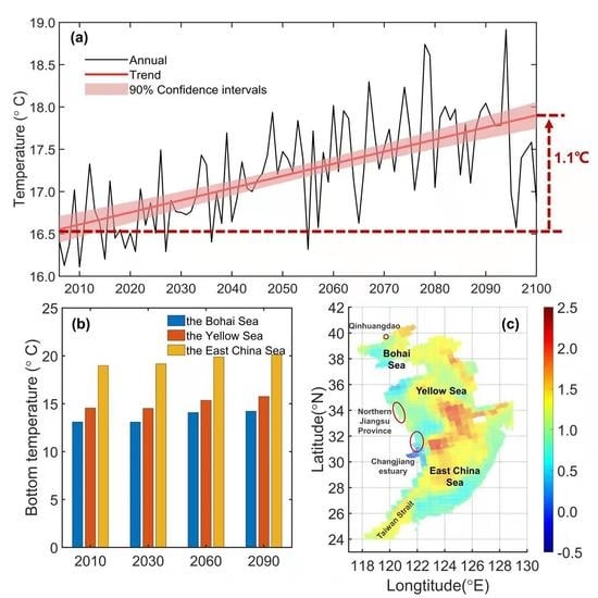
Figure 1.
The essential ideas and findings of this paper are as follows: (a) the projection of interannual SBT from 2006 to 2100 using MPI-ESM-MR under RCP4.5; (b) the interdecadal changes in SBT for the Bohai Sea, Yellow Sea, and East China Shelf Seas in the 2030s, 2060s, and 2090s compared to the 2010s; (c) the spatial distribution of SBT changes in the 2090s compared to the 2010s.

Figure 2.
Water depth map in the East China Shelf Seas with contours of 0 m, 50 m, 100 m, 150 m, and 200 m.
Figure 2.
Water depth map in the East China Shelf Seas with contours of 0 m, 50 m, 100 m, 150 m, and 200 m.

Figure 3.
Vertical temperature distribution in the Bohai Sea, Yellow Sea, and East China Sea: (a) Bohai Sea; (b) Yellow Sea; (c) East China Sea. The horizontal axis indicates temperature. Vertical axis indicates water depth level: 1 denotes 1–12 m; 2 denotes 12–22 m; 3 denotes 22–32 m; 4 denotes 32–42 m; 5 denotes 42–52 m; 6 denotes 52–62 m; 7 denotes 62–75 m; 8 denotes 75–90 m; 9 denotes 90–110 m; 10 denotes 110–135 m; 11 denotes 135–165 m; 12 denotes 165–200 m; 13 denotes 200–240 m.

Figure 4.
Model validation: Each subfigure indicates the bottom temperature (°C), the horizontal axis denotes the longitude (°E) and the vertical axis denotes the latitude (°N). The first to sixth rows illustrate the results of six CMIP5 models. The final row displays the observational data from WOA18. The first to fifth columns present the results for the entire year and the four seasons of 2010, respectively.

Figure 5.
The error maps of MPI-ESM-MR in 2010 in yearly and seasonal ways: (a) yearly-mean, (b) spring, (c) summer, (d) autumn, and (e) winter.
Figure 5.
The error maps of MPI-ESM-MR in 2010 in yearly and seasonal ways: (a) yearly-mean, (b) spring, (c) summer, (d) autumn, and (e) winter.

Figure 6.
Interannual yearly and seasonal mean SBT changes using MPI-ESM-MR in the ECSSs: the first to fifth rows present the results in the annual and four seasons, respectively. The first to third columns illustrate the results from three seas. Since this figure is mainly used to demonstrate the trend of SBT changes in each sea area, it can be really difficult to illustrate this trend using a unified color bar. Thus, we use various color bars for each sea area. The gray line indicates the trend of SBT changes. The red, blue and yellow lines indicate the results of the linear fit of the SBT changes in the Bohai Sea, Yellow Sea and East China Sea respectively.

Figure 7.
Interdecadal SBT changes of six modified models.

Figure 8.
The interdecadal annual SBT changes projected by MPI-ESM-MR: the annual mean bottom temperature in (a) 2030, (c) 2060, (e) and 2090, as well as their changes compared with that in 2010: (b) 2030–2010, (d) 2060–2010, (f) 2090–2010.
Figure 8.
The interdecadal annual SBT changes projected by MPI-ESM-MR: the annual mean bottom temperature in (a) 2030, (c) 2060, (e) and 2090, as well as their changes compared with that in 2010: (b) 2030–2010, (d) 2060–2010, (f) 2090–2010.

Figure 9.
Interdecadal seasonal projection of SBT variations by MPI-ESM-MR. The first to third columns show the seasonal mean changes from the 2010s to the 2030s, to the 2060s, and to the 2090s, respectively. The first to fourth rows illustrate the changes in the four seasons, respectively.
Figure 9.
Interdecadal seasonal projection of SBT variations by MPI-ESM-MR. The first to third columns show the seasonal mean changes from the 2010s to the 2030s, to the 2060s, and to the 2090s, respectively. The first to fourth rows illustrate the changes in the four seasons, respectively.

Figure 10.
The EOF result of interannual mean from 2006 to 2099 under the first principal dimension using MPI-ESM-MR: (a) the original EOF result; (b) the EOF result of the de-2010 climate state one.
Figure 10.
The EOF result of interannual mean from 2006 to 2099 under the first principal dimension using MPI-ESM-MR: (a) the original EOF result; (b) the EOF result of the de-2010 climate state one.

Figure 11.
The original EOF resultd under the first principal dimension from 2006 to 2099 using MPI-ESM-MR for different seasons: (a) spring, (b) summer, (c) autumn, and (d) winter.
Figure 11.
The original EOF resultd under the first principal dimension from 2006 to 2099 using MPI-ESM-MR for different seasons: (a) spring, (b) summer, (c) autumn, and (d) winter.

Figure 12.
The de-2010 climate state of EOF results under the first principal dimension from 2006 to 2099 using MPI-ESM-MR for different seasons: (a) spring, (b) summer, (c) autumn, and (d) winter.
Figure 12.
The de-2010 climate state of EOF results under the first principal dimension from 2006 to 2099 using MPI-ESM-MR for different seasons: (a) spring, (b) summer, (c) autumn, and (d) winter.


Table 1.
The information of the six CMIP5 models utilized in this paper, including the vertical coordinate type (z, , isopycnic or sigma level), the number of vertical levels, and the horizontal resolution (latitude × longitude), and the references.
Table 1.
The information of the six CMIP5 models utilized in this paper, including the vertical coordinate type (z, , isopycnic or sigma level), the number of vertical levels, and the horizontal resolution (latitude × longitude), and the references.
| Model Name | Vertical Grid | Horizontal Resolution | Reference |
|---|---|---|---|
| ACCESS1.3 | z 50 | 0.3° × 1.0° | [35] |
| CCSM4 | z 60 | 0.5° × 1.1° | [36] |
| FIO-ESM | z 40 | 0.5° × 1.1° | [37] |
| CESM1-WACCM | z 60 | 0.5° × 1.1° | [38] |
| NorESM1-ME | z 70 | 0.5° × 1.1° | [39] |
| MPI-ESM-MR | z 40 | 0.1° × 0.1° | [40] |
Table 2.
Model validation of temperatures by comparing the data from each CMIP5 model with the WOA18 observation data in 2010 (°C).
Table 2.
Model validation of temperatures by comparing the data from each CMIP5 model with the WOA18 observation data in 2010 (°C).
| Data Source | Yearly-Mean | Spring | Summer | Autumn | Winter | |
|---|---|---|---|---|---|---|
| WOA18 | 14.76 | 13.47 | 17.87 | 16.63 | 16.40 | |
| CMIP5 Model Errors | ACCESS1.3 | 0.69 | 0.65 | 1.40 | 1.30 | 0.83 |
| CCSM4 | 0.74 | 0.83 | 1.30 | 1.26 | 0.91 | |
| FIO-ESM | 1.16 | 0.67 | 0.95 | 1.71 | 1.32 | |
| CESM1-WACCM | 1.21 | 0.96 | 0.37 | 1.37 | 2.14 | |
| NorESM1-ME | 0.87 | 0.84 | 1.15 | 1.30 | 1.16 | |
| MPI-ESM-MR | 0.77 | 0.33 | 0.30 | 1.22 | 1.21 | |
Table 3.
Interannual and seasonal bottom temperature changes of MPI-ESM-MR in the ECSSs (°C).
| SBT Changes (2100–2006) | Ann. | Spr. | Sum. | Aut. | Win. |
|---|---|---|---|---|---|
| Bohai Sea | 1.60 | 1.92 | 1.75 | 1.36 | 1.45 |
| Yellow Sea | 1.49 | 1.63 | 1.55 | 1.43 | 1.44 |
| East China Sea | 1.21 | 1.36 | 1.11 | 1.08 | 1.38 |
Table 4.
Interdecadal SBT changes of six models across the entire region of the ECSSs (°C).
| SBT | 2010s | 2030s | 2060s | 2090s |
|---|---|---|---|---|
| ACCESS1.3 | 14.62 | 15.37 | 16.75 | 17.23 |
| CCSM4 | 14.60 | 14.70 | 15.58 | 15.45 |
| FIO-ESM | 14.73 | 14.92 | 15.02 | 14.89 |
| CESM1-WACCM | 14.70 | 14.64 | 14.90 | 15.23 |
| NorESM1-ME | 14.60 | 14.14 | 15.21 | 15.36 |
| MPI-ESM-MR | 14.59 | 14.67 | 15.45 | 15.77 |
| Average | 14.63 | 14.90 | 16.05 | 16.19 |
| SBT changes | 2010 | 2030–2010 | 2060–2010 | 2090–2010 |
| change rate | (2030–2010)/years | (2060–2030)/years | (2090–2060)/years | |
| ACCESS1.3 | 14.62 | 0.75 | 2.13 | 2.61 |
| 0.036 | 0.045 | 0.015 | ||
| CCSM4 | 14.60 | 0.10 | 0.98 | 0.85 |
| 0.005 | 0.028 | −0.004 | ||
| FIO-ESM | 14.73 | 0.18 | 0.29 | 0.15 |
| 0.009 | 0.003 | −0.004 | ||
| CESM1-WACCM | 14.70 | −0.06 | 0.20 | 0.53 |
| −0.003 | 0.009 | 0.011 | ||
| NorESM1-ME | 14.60 | −0.46 | 0.60 | 0.76 |
| −0.022 | 0.034 | 0.005 | ||
| MPI-ESM-MR | 14.59 | 0.09 | 0.86 | 1.18 |
| 0.004 | 0.025 | 0.010 | ||
| Average | 14.63 | 0.27 | 1.43 | 1.56 |
| 0.013 | 0.037 | 0.004 |
Table 5.
Interdecadal seasonal SBT changes of six modified models (°C).
| SBT | 2010s | 2030s | 2060s | 2090s | ||||||||||||
|---|---|---|---|---|---|---|---|---|---|---|---|---|---|---|---|---|
| Spr. | Sum. | Aut. | Win. | Spr. | Sum. | Aut. | Win. | Spr. | Sum. | Aut. | Win. | Spr. | Sum. | Aut. | Win. | |
| ACCESS1.3 | 13.25 | 17.38 | 16.58 | 11.27 | 13.82 | 17.97 | 17.53 | 12.17 | 15.28 | 19.79 | 19.00 | 12.95 | 15.66 | 20.19 | 19.50 | 13.56 |
| CCSM4 | 13.20 | 17.40 | 16.62 | 11.18 | 13.20 | 17.53 | 16.83 | 11.25 | 14.23 | 18.35 | 17.54 | 12.21 | 13.95 | 18.36 | 17.71 | 11.79 |
| FIO-ESM | 13.36 | 17.49 | 16.71 | 11.36 | 13.60 | 17.68 | 16.67 | 11.71 | 13.61 | 17.81 | 16.99 | 11.67 | 13.46 | 17.77 | 16.92 | 11.38 |
| CESM1-WACCM | 13.32 | 17.46 | 16.69 | 11.33 | 13.29 | 17.40 | 16.68 | 11.19 | 13.43 | 17.72 | 17.09 | 11.37 | 13.73 | 18.06 | 17.35 | 11.78 |
| NorESM1-ME | 13.22 | 17.41 | 16.61 | 11.17 | 12.71 | 17.05 | 16.39 | 10.43 | 13.87 | 18.19 | 17.47 | 11.29 | 13.93 | 18.44 | 17.62 | 11.46 |
| MPI-ESM-MR | 13.26 | 17.45 | 16.53 | 11.11 | 13.20 | 17.45 | 16.59 | 11.46 | 13.96 | 18.35 | 17.50 | 11.99 | 14.56 | 18.61 | 17.48 | 12.44 |
| Average | 13.22 | 17.63 | 16.63 | 11.02 | 13.40 | 17.89 | 16.96 | 11.34 | 14.64 | 19.19 | 18.16 | 12.23 | 14.70 | 19.35 | 18.36 | 12.34 |
| SBT Changes | 2010s | 2030s–2010s | 2060s–2010s | 2090s–2010s | ||||||||||||
| Spr. | Sum. | Aut. | Win. | Spr. | Sum. | Aut. | Win. | Spr. | Sum. | Aut. | Win. | Spr. | Sum. | Aut. | Win. | |
| ACCESS1.3 | 13.25 | 17.38 | 16.58 | 11.27 | 0.57 | 0.58 | 0.95 | 0.90 | 2.02 | 2.41 | 2.41 | 1.69 | 2.40 | 2.81 | 2.92 | 2.30 |
| CCSM4 | 13.20 | 17.40 | 16.62 | 11.18 | 0.01 | 0.12 | 0.21 | 0.06 | 1.03 | 0.95 | 0.92 | 1.03 | 0.75 | 0.96 | 1.09 | 0.60 |
| FIO-ESM | 13.36 | 17.49 | 16.71 | 11.36 | 0.24 | 0.19 | −0.04 | 0.35 | 0.24 | 0.31 | 0.28 | 0.31 | 0.10 | 0.28 | 0.02 | 0.02 |
| CESM1-WACCM | 13.32 | 17.46 | 16.69 | 11.33 | −0.03 | −0.06 | −0.01 | −0.14 | 0.10 | 0.26 | 0.40 | 0.05 | 0.41 | 0.60 | 0.66 | 0.45 |
| NorESM1-ME | 13.22 | 17.41 | 16.61 | 11.17 | −0.51 | −0.36 | −0.21 | −0.75 | 0.65 | −0.78 | 0.86 | 0.11 | 0.74 | 1.03 | 1.01 | 0.29 |
| MPI-ESM-MR | 13.26 | 17.45 | 16.53 | 11.11 | −0.06 | 0.00 | 0.06 | 0.35 | 0.70 | 0.89 | 0.97 | 0.88 | 1.30 | 1.15 | 0.95 | 1.33 |
| Average | 13.22 | 17.63 | 16.63 | 11.02 | 0.18 | 0.25 | 0.33 | 0.32 | 1.42 | 1.56 | 1.52 | 1.21 | 1.48 | 1.72 | 1.73 | 1.32 |
Table 6.
The annual and seasonal correlations between the mean Taiwan Warm Current bottom temperature and the SBT in the outer shelf of the East China Sea (the first row); the correlation between the Kuroshio water flux and the SBT in the outer shelf of the East China Sea (the second row).
Table 6.
The annual and seasonal correlations between the mean Taiwan Warm Current bottom temperature and the SBT in the outer shelf of the East China Sea (the first row); the correlation between the Kuroshio water flux and the SBT in the outer shelf of the East China Sea (the second row).
| Impact Factor | Annual | Spring | Summer | Autumn | Winter |
|---|---|---|---|---|---|
| Taiwan Warm Current SBT | 0.57 | 0.58 | 0.49 | 0.38 | 0.07 |
| Kuroshio water flux | −0.41 | −0.39 | −0.63 | −0.56 | −0.42 |
Table 7.
The annual and seasonal average SBTs of the Taiwan Warm Current and Kuroshio from 2006 to 2100 (°C).
Table 7.
The annual and seasonal average SBTs of the Taiwan Warm Current and Kuroshio from 2006 to 2100 (°C).
| Critical Ocean Current | Annual | Spring | Summer | Autumn | Winter |
|---|---|---|---|---|---|
| Taiwan Warm Current Average SBT | 24.62 | 23.86 | 26.76 | 26.49 | 21.37 |
| Kuroshio Average SBT | 18.07 | 17.91 | 17.68 | 17.77 | 18.91 |
Disclaimer/Publisher’s Note: The statements, opinions and data contained in all publications are solely those of the individual author(s) and contributor(s) and not of MDPI and/or the editor(s). MDPI and/or the editor(s) disclaim responsibility for any injury to people or property resulting from any ideas, methods, instructions or products referred to in the content. |
© 2023 by the authors. Licensee MDPI, Basel, Switzerland. This article is an open access article distributed under the terms and conditions of the Creative Commons Attribution (CC BY) license (https://creativecommons.org/licenses/by/4.0/).
Share and Cite
MDPI and ACS Style
Qiao, S.; Zhang, C.; Wei, H.; Lan, Y. Projected Sea Bottom Temperature Variability in the East China Shelf Seas by 2100. J. Mar. Sci. Eng. 2023, 11, 1192. https://doi.org/10.3390/jmse11061192
AMA Style
Qiao S, Zhang C, Wei H, Lan Y. Projected Sea Bottom Temperature Variability in the East China Shelf Seas by 2100. Journal of Marine Science and Engineering. 2023; 11(6):1192. https://doi.org/10.3390/jmse11061192
Chicago/Turabian StyleQiao, Shen, Cuicui Zhang, Hao Wei, and Yifan Lan. 2023. "Projected Sea Bottom Temperature Variability in the East China Shelf Seas by 2100" Journal of Marine Science and Engineering 11, no. 6: 1192. https://doi.org/10.3390/jmse11061192
Note that from the first issue of 2016, this journal uses article numbers instead of page numbers. See further details here.