A Coupled Hydrodynamic–Structural Model for Flexible Interconnected Multiple Floating Bodies

Abstract

Evaluating the structural safety and seakeeping performance of very large floating structures (VLFS) using the rigid module flexible connector (RMFC) method remains challenging due to the complexity of the coupled hydrodynamic–structural responses in this system. In this study, a coupled hydrodynamic–structural frequency–time domain model is developed based on the RMFC method employing the planar Euler–Bernoulli beam elements to investigate the dynamic responses of multi-module floating systems. To reveal the dynamic characteristics of the systems, the coupled hydrodynamic–structural responses are investigated using a frequency–time-domain numerical model with viscous correction, in which the mass and stiffness attributes of connectors are incorporated into the system. Given the effects of hydrodynamic interaction, consideration is given to the case of three modular boxes connected by flexible beams aligned in series in shallow water to validate the present model. Higher efficiency and accuracy can be found in the system using viscous correction in potential flow theory and introducing state–space model to replace the convolution terms in the Cummins equation for the time domain. Moreover, this model can be extended to a considerable number of floating modules, which provides possibilities to analyze N-module floating systems.

1. Introduction

With the acceleration of the exploitation of ocean resources, multiple floaters near offshore operations are becoming more common, such as multi-module floating systems [1], offloading operations from FLNG to LNG carrier [2,3], offshore platform float-over deck installations [4,5,6] and floating wind–wave power-generation platforms [7,8]. These systems may experience strong hydrodynamic interactions, resulting in enormous wave loads generated in the gaps between two floaters. On the other hand, the multi-module floating system has become increasingly prosperous in offshore activities due to the need for large size and the functional integration of floating structures, e.g., the MOB (mobile offshore base) [9,10,11] and floating airports [12]. Such structures require a high degree of integrity, due to the complex hydrodynamic interactions and dynamic interactions between different modules via the connectors [13,14]. Additional attention should therefore be paid to mitigating the relative movements of adjacent modules in the system subjected to environmental load. Therefore, the assessment of the coupling dynamic effects of the interconnected multi-module floating system is of paramount importance to improving the safety and the seakeeping performance of offshore structures operating in the form of adjacent multiple floating bodies. Since much literature has been dedicated to investigating the effect of hydrodynamic interactions, such as gap resonance [6,15,16,17,18], this study will concentrate on developing a coupled hydrodynamic–structural frequency–time-domain model based on the previous work by Chen et al. [1].

Connectors can be classified into rigid ones and flexible ones according to their characteristics. Rigid connectors between modules are usually welded and hinged, which are characterized by simple structure and easy manufacture. However, rigid connectors are unable to release the bending stress and shear stress induced by the large deflection of the system, resulting in prominent fatigue problems and short service life. To avoid excessive stress caused by rigid connectors, research on flexible connectors has gained prosperity in recent years. The structural dynamic responses of the interconnected multi-module system are generally investigated using the rigid module flexible connector (RMFC) method. In this method, it is assumed that the stiffness of connectors is much smaller than that of the floating modules; meanwhile, structural deformation occurs on the connector while the modules themself do not deform.

Ever since the concept of very large floating structures (VLFS) was put forward, various connector designs have been proposed by scholars worldwide. Some previous connector designs for VLFS were summarized by Jiang et al. [19]. In some sea conditions, the natural frequency of the overall system is close to that of the connectors, which may result in large relative responses of the floating bodies and further dangerous overloading of the connectors [20]. To reduce loads on the connectors, Haney [21] proposed several compliant connector configurations. On top of this, the designs using rubber cushions and cables [22,23] and using springs [24,25,26] were generally applied to provide flexible connections. On this basis, Qi et al. [27] and Zhang et al. [28] investigated, respectively, the use of ball–spring devices and nylon–rubber materials in the design of a flexible connector.

Apart from proposing new designs for a connector, scholars are also dedicated to investigating the characteristics of dynamic responses of the multi-module system using the RMFC method both experimentally and numerically. Three-dimensional experiments were conducted by Loukogeorgaki et al. [29] to investigate flexible connectors’ internal forces of a pontoon-type multi-module floating system. Ding et al. [30] carried out both experimental and numerical analyses to investigate the RMFC model. Michailides et al. [31] developed a numerical analysis framework to evaluate connectors’ internal loads and further optimize the configuration of a modular pontoon-type floating structure. Yang et al. [32] established a three-step time-domain method to assess the motions of each module and connector load based on the Boussinesq equation and Cummins equation. Bispo et al. [33,34] investigated the wave interactions of multi-floating systems with articulated and hinged connections using the potential-flow-based model and analytical models. Chen et al. [5] developed a hydrodynamic–structural frequency-domain model by combining the dynamic substructuring method and static condensation as well as considering the flexibility of connectors and hydrodynamic interactions to analyze the catamaran tow operation in the Spar float-over deck installation scenario. The frequency–time-domain method was first proposed by Cummins [35], and this method has been adopted in standard software, such as AQWA [36,37,38].

The connector load and module motion are two key indicators to evaluate the safety and seakeeping performance of the system. Wang et al. [39] found that connector stiffness is the most important factor affecting relative motion and load conditions. Fu et al. [13] further proved that the stiffness of flexible connectors has a great influence on the hydroelastic responses of the multi-floating system. By comparing connectors with different stiffness, Gao et al. [14] suggested that proper stiffness can effectively reduce hydroelastic responses in the system. Wang et al. [40] carried out a parametric study to investigate the connector characteristics, and appropriate stiffness and damping coefficients have been demonstrated to release the load while retaining reasonable relative motion between adjacent modules. On the other hand, the high-efficiency time-domain analysis model is one of the research interests. The State–Space Model (SSM) is widely used in analyzing marine operations, which has proven to be more efficient than directly solving the Cummins equation with a convolution term. Chen et al. [41,42,43] and Zou et al. [44] proposed a constant-parameter time-domain model (CPTDM) by replacing the convolution terms in the Cummins equation with SSMs to investigate the complex dynamics in the float-over deck installation for a jacket platform with a single barge. This method was then further developed to analyze other marine operation systems, such as multi-floater float-over systems [6,45] and marine renewable energy devices [46]. However, due to the limitation of current analysis methods, the RMFC model usually requires simplification, such as using springs and dampers to replace the connection component. From the aforementioned study, a brief conclusion can be drawn that connector loads and module motions are significantly influenced by connector stiffness and damping coefficients. Therefore, it is of great necessity to develop a robust and efficient coupled frequency–time-domain model for a multi-module floating system, which can consider connector flexibility.

In this study, a hydrodynamic–structural model for an interconnected multi-module floating system is developed, which is based on the hydrodynamic results obtained from the common hydrodynamic analysis code, e.g., the commercial code AQWA. At the same time, to eliminate the adverse effects of distortion of hydrodynamic resonance obtained in the potential flow theory system on the results, the damping lid method [1,6,47,48] is used for viscous correction. The frequency-domain simulations are first verified with the results calculated by AQWA in the free-floating status. When further considering the connector system, the effects of the bending stiffness of the connectors are investigated, since the corresponding frequency-domain model has been validated in previous studies [49,50,51]. Based on the frequency-domain results, the constant-parameter hydrodynamic–structural time-domain model is established for a multi-module floating system connected end to end and the accuracy of the developed time-domain model is comprehensively discussed.

The paper is arranged as follows. Section 2 introduces the methodology for developing the hydrodynamic–structural model in the frequency domain and time domain. Section 3 discusses the application of the developed numerical model with a three-module system connected end to end, in which the influences of the connector parameters on the overall system behavior are also investigated. Finally, some concluding remarks are given in Section 4.

2. Materials and Methods

2.1. Frequency-Domain Model

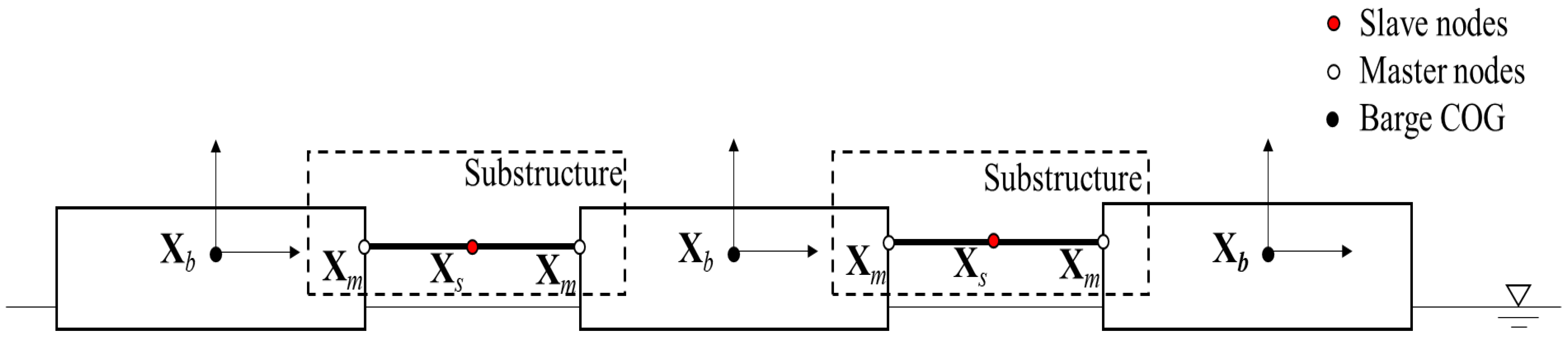
In this research, a hydrodynamic–structural analysis model has been used to analyze the dynamics characteristics in the series of multiple floating systems based on the two-stage method proposed by Sun et al. [49,50,51]. In the first stage, a commercial boundary element method (BEM) code, ANSYS-AQWA, is employed to calculate the first-order wave excitation forces and hydrodynamic coefficients. In the second stage, the dynamic model for the multi-module floating system with flexible connections is established, which is schematically shown in Figure 1. As illustrated in Figure 1, the motions of the barges are indicated as X_b, the motions of the action point between the flexible substructures and barges are defined as master DOF (degrees of freedom), and the nodal motions on the substructures are deemed as slave DOF, which are designated as X_m and X_s, respectively. The establishment of this dynamic model can help to condense the flexible substructures to the barges through master nodes in the form of a condensed mass and stiffness matrix using static condensation; therefore, the wave-induced dynamics of the interconnected system can be conveniently obtained.

By assuming that the only external forces on the substructure are the constraint forces F_m(t) at the connections, the motion equation for the substructure can be written in the following form [52,53]:

$$\left[\begin{array}{cc}{M}_{mm}& M_{ms}\\ M_{ms}^T& M_{ss}\end{array}\right]\left\{\begin{array}{c}{\ddot{X}}_m\left(t\right)\\ {\ddot{X}}_s\left(t\right)\end{array}\right\}+\left[\begin{array}{cc}{K}_{mm}& K_{ms}\\ K_{ms}^T& K_{ss}\end{array}\right]\left\{\begin{array}{c}{X}_m\left(t\right)\\ X_s\left(t\right)\end{array}\right\}=\left\{\begin{array}{c}{F}_m\left(t\right)\\ 0\end{array}\right\}$$

(1)

where the subscripts m and s represent master and slave DOF, respectively, and the superscript T denotes transpose.

In this state, the displacement and acceleration of the flexible substructure can be expressed as:

$$X\left(t\right)=\left\{\begin{array}{c}{X}_m\left(t\right)\\ X_s\left(t\right)\end{array}\right\}; \ddot{X}\left(t\right)=\left\{\begin{array}{c}{\ddot{X}}_m\left(t\right)\\ {\ddot{X}}_s\left(t\right)\end{array}\right\}$$

(2)

Since the resonance responses of the flexible structure itself are not taken into account, the damping terms can be further ignored. Therefore, the second term in the equation can be written as:

$$M_{ms}^T{\ddot{X}}_m\left(t\right)+M_{ss}{\ddot{X}}_s\left(t\right)+K_{ms}^T{X}_m\left(t\right)+K_{ss}{X}_s\left(t\right)=0$$

(3)

Further ignoring the influence of inertia force, the slave DOF $X_s$ and the acceleration vector ${\ddot{X}}_s$ can be expressed by the master DOF $X_m$ and ${\ddot{X}}_m$ in the following form:

$$X_s\left(t\right)=-K_{ss}^{-1}{K}_{ms}^T{X}_m\left(t\right)=T_{ms}^T{X}_m\left(t\right)$$

(4)

$${\ddot{X}}_s\left(t\right)=T_{ms}^T{\ddot{X}}_m\left(t\right)$$

(5)

where $T_{ms}^T$ is the coordinate transformation matrix.

On this basis, the equation of the displacement and acceleration of the substructure can be rewritten as:

$$X\left(t\right)=\left[\begin{array}{c}I\\ T_{ms}^T\end{array}\right]X_m\left(t\right)=T_G{X}_m\left(t\right); \ddot{X}\left(t\right)=\left[\begin{array}{c}I\\ T_{ms}^T\end{array}\right]{\ddot{X}}_m\left(t\right)=T_G{\ddot{X}}_m\left(t\right)$$

(6)

where I denotes the identity matrix and T_G is the transpose matrix.

Substituting Equation (6) into Equation (1) leads to:

$$\left(M_{mm}+M_{ms}{T}_{ms}^T+T_{ms}{M}_{ms}^T+T_{ms}{M}_{ss}{T}_{ms}^T\right){\ddot{X}}_m\left(t\right)+\left(K_{mm}+K_{ms}{T}_{ms}^T\right)X_m\left(t\right)=F_m\left(t\right)$$

(7)

Therefore, an analytical equation involving the master DOF and the constraining force on the master nodes only is constructed. The mass and stiffness matrix on the master nodes of the substructures can be expressed as follows:

$$M_{mm}^{\ast }=M_{mm}+M_{ms}{T}_{ms}^T+T_{ms}{M}_{ms}^T+T_{ms}{M}_{ss}{T}_{ms}^T$$

(8)

$$K_{mm}^{\ast }=K_{mm}+K_{ms}{T}_{ms}^T$$

(9)

The harmonic responses of multiple hydrodynamic interacting structures can be obtained by solving linear equations in linear potential flow theory, which are commonly referred to as Response Amplitude Operators (RAOs). The motions of N floating structures under free-floating conditions can be expressed by frequency-dependent hydrodynamic coefficients as follows:

$$\widehat{X_b}(i\omega )={\widehat{F}}_b^E(i\omega )/\left\{-{\omega }^2\left[M+A_H(\omega )\right]-i\omega B_H(\omega )+C_{bb}\right\}$$

(10)

where $\widehat{X}(i\omega )$ represents the 6N × 1 complex vector of multiple bodies’ RAOs; N is the number of bodies; M, $A_H(\omega )$ and $B_H(\omega )$ are the (6N) × (6N) structural mass, hydrodynamic added mass, and added damping matrices, respectively; $C_{bb}$ is the hydrostatic stiffness matrix assembled by each 6 × 6 sub-hydrostatic stiffness of individual structure along the diagonal; ${\widehat{F}}_{}^E(i\omega )$ is the 6N × 1 wave excitation force at frequency ω.

On this basis, by taking the Fourier transform of both sides of Equation (7), the frequency-domain response equation of rigid floating modules with a flexible connection can be written as:

$$\begin{array}{l}\left\{-{\omega }^2\left[M_{bb}+A_H\left(\omega \right)+T_{bm}{M}_{mm}^{\ast }{T}_{bm}^T+i\omega \left[B_H\left(\omega \right)+B_{\upsilon }\right]+\left(C_{bb}+T_{bm}{K}_{mm}^{\ast }{T}_{bm}^T\right)\right]\right\}\\ ·{\widehat{X}}_b\left(i\omega \right)={\widehat{F}}_b^E\left(i\omega \right)\end{array}$$

(11)

The above equation provides the ability to solve the motion response and constraint force of the master DOF on the flexible structure while solving the RAOs of the rigid barges with connections. The expressions are as follows:

$${\widehat{X}}_m\left(i\omega \right)={\mathrm{T}}_{{}_{bm}}^T{\widehat{X}}_b\left(i\omega \right)$$

(12)

$${\widehat{F}}_m(i\omega )=\left(-{\omega }^2{M}_{mm}^{*}{T}_{bm}^T+K_{mm}^{*}{T}_{bm}^T\right){\widehat{X}}_b(i\omega )$$

(13)

To develop the structural dynamic model in the frequency domain, the connectors are considered to be Euler–Bernoulli beams. When considering the motions in a two-dimensional plane projected on the side of the system, the motions of the two nodes at both ends of the space beam element can be simplified as the translation of the x and z axes and the rotation about the y axis, a total of 6 degrees of freedom, which is shown in Figure 2. According to structural mechanics, the 6-DOF stiffness matrix of a beam element moving in the two-dimensional plane is defined as:

$$\mathrm{K}=[\begin{array}{cccccc}\frac{EA}{l}& & & & & \\ 0& \frac{12E{I}_z}{l^3\left(1+{\Phi }_{\nu }\right)}& & & \hfill \mathrm{Symmetric}\hfill \\ 0& \frac{6E{I}_z}{l^2\left(1+{\Phi }_{\nu }\right)}& \frac{\left(4+{\Phi }_z\right)E{I}_z}{l\left(1+{\Phi }_{\nu }\right)}& & \\ -\frac{EA}{l}& 0& 0& \frac{EA}{l}& \\ 0& \frac{-12E{I}_z}{l^3\left(1+{\Phi }_{\nu }\right)}& \frac{-6E{I}_z}{l^2\left(1+{\Phi }_{\nu }\right)}& 0& \frac{12E{I}_z}{l^3\left(1+{\Phi }_{\nu }\right)}\hfill \\ 0& \frac{6E{I}_z}{l^2\left(1+{\Phi }_{\nu }\right)}& \frac{\left(2-{\Phi }_z\right)E{I}_z}{l\left(1+{\Phi }_{\nu }\right)}& 0& \frac{-6E{I}_z}{l^2\left(1+{\Phi }_{\nu }\right)} \frac{\left(4+{\Phi }_z\right)E{I}_z}{l\left(1+{\Phi }_{\nu }\right)}\end{array}]$$

(14)

Since the Euler–Bernoulli beams used in this model are based on the plane-section assumption, the effect of transverse shear force is therefore ignored. ${\Phi }_{\nu }$ and ${\Phi }_z$ in the matrix above can be viewed as zero, and it can be therefore further simplified as:

$$\mathrm{K}=\frac{E{I}_z}{l^3}\left[\begin{array}{cccc}\frac{A{l}^2}{I_z}& & & \\ 0& 12& & \hfill \mathrm{Symmetric}\hfill \\ 0& 6l& 4l^2& \\ -\frac{A{l}^2}{I_z}& 0& 0& \frac{A{l}^2}{I_z}\hfill \\ 0& -12& -6l& 0 12\hfill \\ 0& 6l& 2l^2& 0 -6l 4l^2\hfill \end{array}\right]$$

(15)

Considering that the mass distribution of the beam element is uniform, its mass matrix form can be obtained according to structural dynamics:

$$\mathrm{M}=\frac{\overline{m}L}{420}\left[\begin{array}{cccc}156& 22L& 54& -13L\\ 22L& 4L^2& 13L& -3L^2\\ 54& 13L& 156& -22L\\ -13L& -3L^2& -22L& 4L^2\end{array}\right]$$

(16)

Furthermore, the Euler–Bernoulli beam element can be used to obtain the condensed mass and stiffness matrix of the horizontal beam at each node using static condensation, in which the mass matrix contained in Equation (8) can be expressed as:

$${\mathrm{M}}_{mm}=\frac{\overline{m}L}{420}\left[\begin{array}{cccccc}140& 0& 0& 0& 0& 0\\ 0& 156& 22L& 0& 0& 0\\ 0& 22L& 4L^2& 0& 0& 0\\ 0& 0& 0& 140& 0& 0\\ 0& 0& 0& 0& 156& -22L\\ 0& 0& 0& 0& -22L& 4L^2\end{array}\right]$$

(17)

$${\mathrm{M}}_{ms}=\frac{\overline{m}L}{420}\left[\begin{array}{cccc}70& 0& 0& 0\\ 0& 54& -13L& 0\\ 0& 13L& -3L^2& 0\\ \begin{array}{c}\begin{array}{c}70\\ 0\end{array}\\ 0\end{array}& \begin{array}{c}\begin{array}{c}0\\ 54\end{array}\\ -13L\end{array}& \begin{array}{c}0\\ 0\\ 0\end{array}& \begin{array}{c}0\\ 13L\\ -3L^2\end{array}\end{array}\right]$$

(18)

$${\mathrm{M}}_{ss}=\frac{\overline{m}L}{420}\left[\begin{array}{cccc}280& 0& 0& 0\\ 0& 312& -22L& 22L\\ 0& -22L& 4L^2& 0\\ 0& 22L& 0& 4L^2\end{array}\right]$$

(19)

In the same way, the stiffness matrices contained in Equation (9) have the following form:

$${\mathrm{K}}_{mm}=\left[\begin{array}{cccccc}EA/L& 0& 0& 0& 0& 0\\ 0& 12EI/L^3& 6EI/L^2& 0& 0& 0\\ 0& 6EI/L^2& 4EI/L& 0& 0& 0\\ 0& 0& 0& EA/L& 0& 0\\ 0& 0& 0& 0& 12EI/L^3& -6EI/L^2\\ 0& 0& 0& 0& -6EI/L^2& 4EI/L\end{array}\right]$$

(20)

$${\mathrm{K}}_{ms}=\left[\begin{array}{cccc}-EA/L& 0& 0& 0\\ 0& -12EI/L^3& 6EI/L^2& 0\\ 0& -6EI/L^2& 2EI/L& 0\\ \begin{array}{c}-EA/L\\ 0\\ 0\end{array}& \begin{array}{c}0\\ -12EI/L^3\\ 6EI/L^2\end{array}& \begin{array}{c}0\\ 0\\ 0\end{array}& \begin{array}{c}0\\ -6EI/L^2\\ 2EI/L\end{array}\end{array}\right]$$

(21)

$${\mathrm{K}}_{ss}=\left[\begin{array}{cccc}2EA/L& 0& 0& 0\\ 0& 24EI/L^3& -6EI/L^2& 6EI/L^2\\ 0& -6EI/L^2& 4EA/L+C& -C\\ 0& 6EI/L^2& -C& 4EA/L+C\end{array}\right]$$

(22)

When the stiffness of the joint is non-zero, it corresponds to the case of a semi-rigid connection, while when the stiffness C is zero, it can be considered to be the case of a hinged connection.

2.2. Coupled Time-Domain Model

Since the frequency-domain method is based on linear potential theory, the nonlinearities of the multi-module floating system with connectors are not able to be evaluated. The time-domain model described by the Cummins equation [35] has been widely used in analyzing the nonlinear dynamics of various types of marine multi-floater systems, such as the floating wind–wave power generation platform, catamaran float-over deck installation and multi-module floating system. For the case of the freely floating condition with zero forward speed, the Cummins equation can be written as:

$$\left[M+A_H(\infty )\right]{\ddot{X}}_b(t)+{\displaystyle \underset{0}{\overset{t}{\int }}K(t-\tau ){\dot{X}}_b(\tau )d\tau +C_{bb}{X}_b(t)}=F_b^E(t)$$

(23)

where $F^E(t)$ denotes the time-domain wave excitation forces, $K(t)$ and $A_H(\infty )$ is the matrix of the impulse response functions and added mass at infinite frequency, respectively, which can be obtained from the frequency-domain results [54]:

$$\begin{array}{l}K(t)=\frac{2}{\pi }{\displaystyle {\int }_0^{\infty }{B}_H\left(\omega \right)\cos \left(\omega t\right)}d\omega \\ A(\infty )=A(\omega )+\frac{1}{\omega }{\displaystyle {\int }_0^{\infty }K(\tau )\sin \left(\omega \tau \right)}d\tau \end{array}$$

(24)

Further consideration is given to the aforementioned cohesion stiffness and mass, the coupling equation considering the flexible connectors in the frequency domain can be transformed to the time domain, which can be written as:

$$\begin{array}{l}\left[M_{bb}+A_H(\infty )+T_{bm}{M}_{mm}^{\ast }{T}_{bm}^T\right]{\ddot{X}}_b\left(t\right)+{\displaystyle \underset{0}{\overset{t}{\int }}K\left(t-\tau \right){\dot{X}}_b\left(\tau \right)\mathrm{d}\tau }+\\ \left[C_{bb}+T_{bm}{K}_{mm}^{\ast }{T}_{bm}^T\right]X_b\left(t\right)=F_b^E\left(t\right)\end{array}$$

(25)

When solving the Cummins equation, the convolution term with kernel function K(t) within the time range from 0 to t is calculated at each time step, therefore the integrating process is time-consuming and easy to accumulate and amplify errors. Since the convolution term is a linear time-invariant system, one can replace it with either a state–space model or a transfer function to improve its accuracy and efficiency [55]. A single-input–single-output (SISO) state–space model can be easily established to be equivalent to each convolution term [42]. Once the SISO state–space models for all the impulse response functions are obtained, the multi-input–multi-output (MIMO) state–space model replaces the matrix of the convolution terms [43]:

$$\begin{array}{l}\dot{z}(t)=P\ast z(t)+Q\ast \dot{x}(t)\\ Y\left(\dot{x}(t)\right)=S\ast z(t)\end{array}$$

(26)

where z(t) represents the state vector; P, Q, and S are the parametric matrices of the MIMO state–space model, which have the following forms [4]:

$$P=\left[\begin{array}{cccc}{P}_{i1}& 0& \cdots & 0\\ 0& P_{i2}& \cdots & 0\\ 0& 0& \ddots & 0\\ 0& 0& \cdots & P_{iq}\end{array}\right],P\in {\mathrm{R}}^{(q\times n)\times (q\times n)}(i=1,\dots ,q)$$

(27)

$$Q=\left[\begin{array}{cccc}{Q}_{11}& 0& \cdots & 0\\ 0& Q_{12}& \ddots & ⋮\\ ⋮& \ddots & \ddots & 0\\ 0& 0& \cdots & Q_{1q}\\ ⋮& ⋮& ⋮& ⋮\\ Q_{q1}& 0& \cdots & 0\\ 0& Q_{q2}& \ddots & ⋮\\ ⋮& \ddots & \ddots & 0\\ 0& 0& \cdots & Q_{qq}\end{array}\right],Q\in {\mathrm{R}}^{(q\times n)\times q}$$

(28)

$$S=\left[\begin{array}{ccccccc}{S}_{11}& \cdots & S_{1q}& 0& \cdots & \cdots & 0\\ ⋮& ⋮& ⋮& \ddots & ⋮& ⋮& ⋮\\ 0& \cdots & 0& \dots & S_{q1}& \dots & S_{qq}\end{array}\right],S\in {\mathrm{R}}^{(q)\times (q\times n)}$$

(29)

where q denotes the number of degrees of freedom, which is 18 for the three-barge model; k is the order of the individual SISO state–space model.

By replacing the convolution term with the MIMO state–space model, a coupled constant parameter hydrodynamic–structural time-domain model (CPHSTDM) can be established based on the Cummins equation:

$$\begin{array}{l}\left[M_{bb}+A_H(\infty )+T_{bm}{M}_{mm}^{\ast }{T}_{bm}^T\right]{\ddot{X}}_b\left(t\right)+Y\left(\dot{x}(t)\right)+\\ \left[C_{bb}+T_{bm}{K}_{mm}^{\ast }{T}_{bm}^T\right]X_b\left(t\right)=F_b^E\left(t\right)\end{array}$$

(30)

It should be noted that the hydrodynamic–structural system described by Equation (30) is significantly more efficient compared to AQWA [6]. In addition, the multi-module floating system to be analyzed in this study involves multi-body hydrodynamic interactions with strong resonant phenomena, which will have a significant effect on the hydrodynamic coefficients, resulting in error generated in the frequency–time-domain transformation. To ensure the error lies within an acceptable threshold, the damping lid method is employed in this study. Detailed information about the damping lid method can be found in works by Zou et al. [6] and Chen et al. [1]. To quantify the fitting quality of the SSMs, the coefficient R² is applied [56]:

$$R^2=1-\frac{{\displaystyle \sum _l^{}{({\hat{\mathrm{K}}}_{i,j}(t_l)-{\tilde{\mathrm{K}}}_{i,j}(t_l))}^2}}{{\displaystyle \sum _l^{}{({\hat{\mathrm{K}}}_{i,j}(t_l)-{\overline{\mathrm{K}}}_{i,j})}^2}}$$

(31)

where ${\tilde{\mathrm{K}}}_{i,j}(t_l)$ denotes the output of the SISO state–space model at time t_l for the input being the Dirac delta function, and ${\overline{\mathrm{K}}}_{i,j}$ is the mean value of ${\hat{\mathrm{K}}}_{i,j}(t)$.

3. Discussion of the Development of CPHSTDM and Parametric Study on Connector Parameters

A three-module floating system aligned in a longitudinal direction is applied to this study in this section, which is based on the numerical study carried out by Chen et al. [1]. The results of the hydrodynamic analysis required in the coupled constant parameter hydrodynamic–structural time-domain model (CPHSTDM) are obtained by the standard panel code ANSYS-AQWA; on this basis, the influence of connector parameter characteristics between modules is further considered, and the characteristics of motion responses and loads of the multi-floating system are analyzed by CPHSTDM, which is subjected to wave forces and connection constraints between modules simultaneously.

3.1. Particulars of the Analyzed Model

The selected floating body module is a box structure with an aspect ratio of 2:1, and its mass distribution is uniform. The particulars of the single floating module in the prototype are summarized in

Table 1. The particulars of the single floating module in the prototype.

Module Characteristic	Value
Length, L(m)	100
Breadth, B(m)	50
Depth (m)	5
Draught, D(m)	2
Center of gravity above base, KG (m)	2.5
Radius of roll gyration, Rxx (m)	14.5
Radius of pitch gyration, Ryy (m)	28.9

. The model to be analyzed in this study remains consistent with Chen et al. [1], in which a series of analyses on a three-module system to investigate the gap resonance phenomenon in shallow water is conducted. Although the previous work mainly investigates the gap resonance phenomenon, this study further investigates the dynamic characteristics of the interconnected three-module floating system with a narrow gap, whose connectors are considered to be Euler–Bernoulli beams.

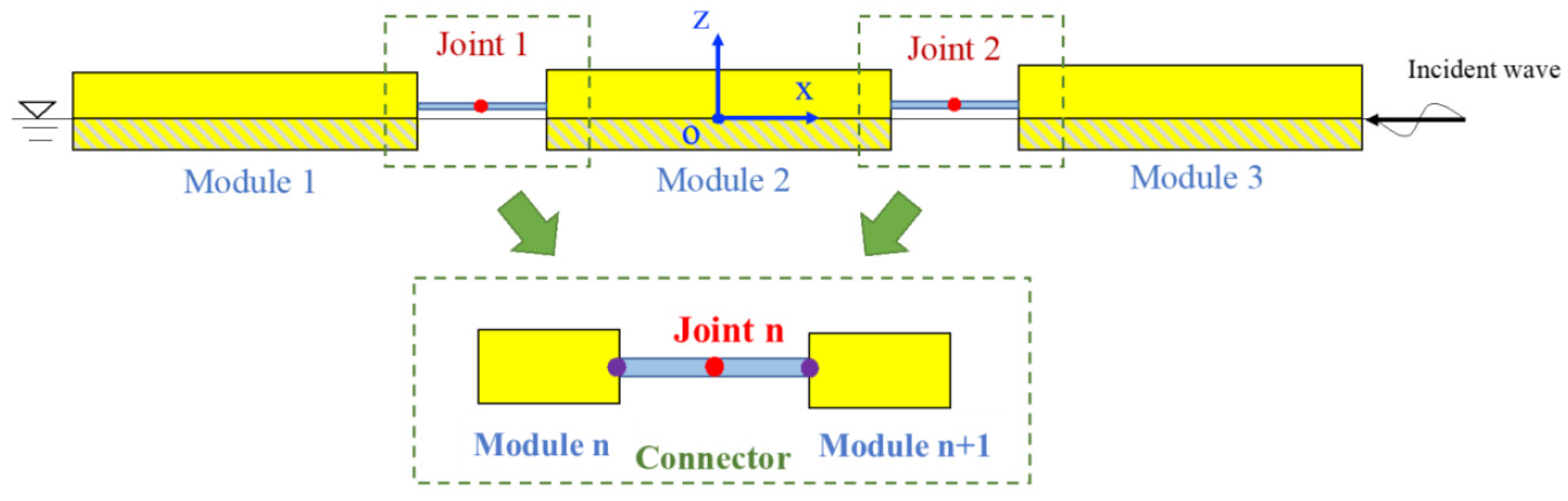
To verify the coupled CPHSTDM, a three-module model, in which adjacent modules are connected end to end, has been analyzed under head sea conditions as illustrated in Figure 3. The water depth is 50 m. As shown in Figure 4, one connector consists of two identical Euler–Bernoulli beams combined through a single joint. The length of each beam is 2.5 m and it is considered that the mass of the beam is uniformly distributed, and the mass of each unit length is taken as 10 kg/m. As mentioned in Section 2, the motion responses at the connecting points on the module are known as X_m, while the motion at the joint is defined as X_s.

3.2. Frequency-Domain Simulations of the Interconnected Three-Module System

First, a full-scale three-module floating system is analyzed using the panel code ANSYS-AQWA in the frequency domain. To meet the accuracy of the subsequent time-domain model calculation, the wave frequencies selected in the process of frequency-domain hydrodynamic analysis cover a wide-enough range from low frequency to high frequency, i.e., from 0.01 rad/s to 2.41 rad/s with a step of 0.05 rad/s to reduce calculation error. According to the analyses conducted by Chen et al. [1] and Zou et al. [6], the overestimated gap resonances can be observed in the multi-module system; therefore, applying the external damping lid on the free surface of the gap fluid is essential, which has been proved to be capable of effectively mitigating the unrealistic resonances. To highlight the multi-body hydrodynamic interactions, the single-module case and three-module case are both calculated in this study.

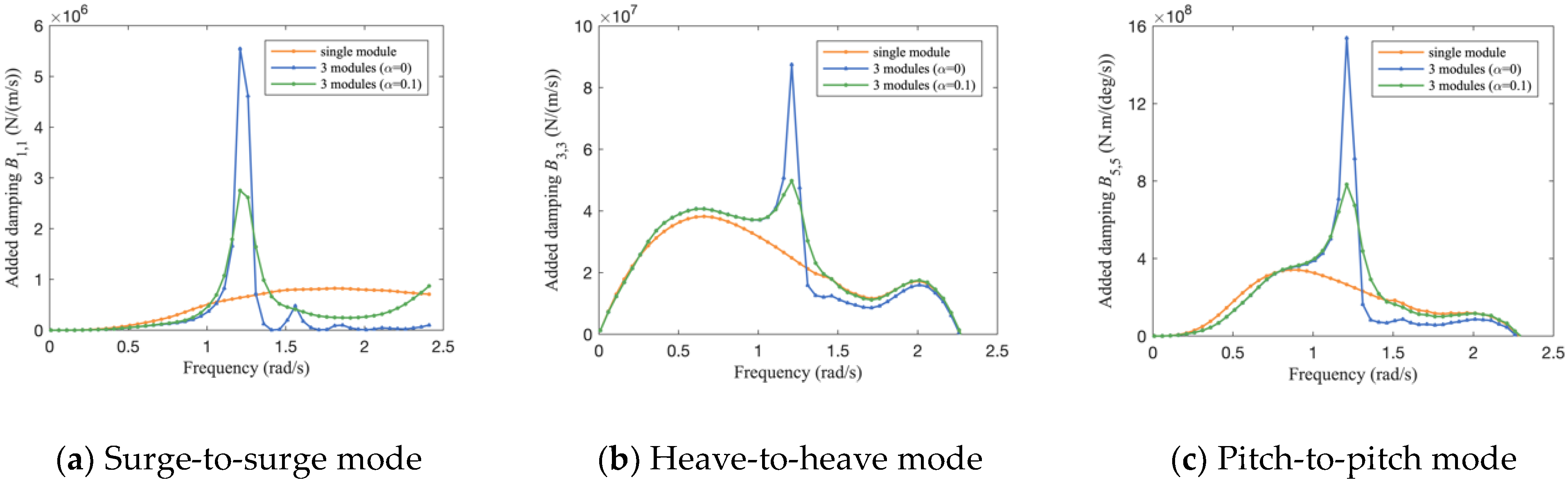
Figure 5 and Figure 6 show part of the hydrodynamic coefficients. It can be seen that, compared with the single-module condition, due to the existence of adjacent floating bodies, the hydrodynamic coefficient of the wave-facing module in the multi-module system has changed significantly, revealing the characteristics of pumping resonance [17]. When the damping factor is zero, it means no viscous correction is introduced into the hydrodynamic analysis. Under the influence of the hydrodynamic interactions, the added mass experiences first a maximum and then a minimum value (sometimes becoming negative); meanwhile, the damping term appears at a certain frequency near the phenomenon of the obvious resonance peak. Considering the recommended damping lid factor, which ranges from 0 to 0.2 [57], and the computability problem of the time-domain model, a damping factor with an intermediate value of 0.1 was selected for analysis in this study to tune the numerical results more realistic while reserving the hydrodynamic interaction characteristics. With the introduction of the damping lid factor, the exorbitant oscillations hydrodynamic coefficient curves are effectively controlled, and the intensity has been improved.

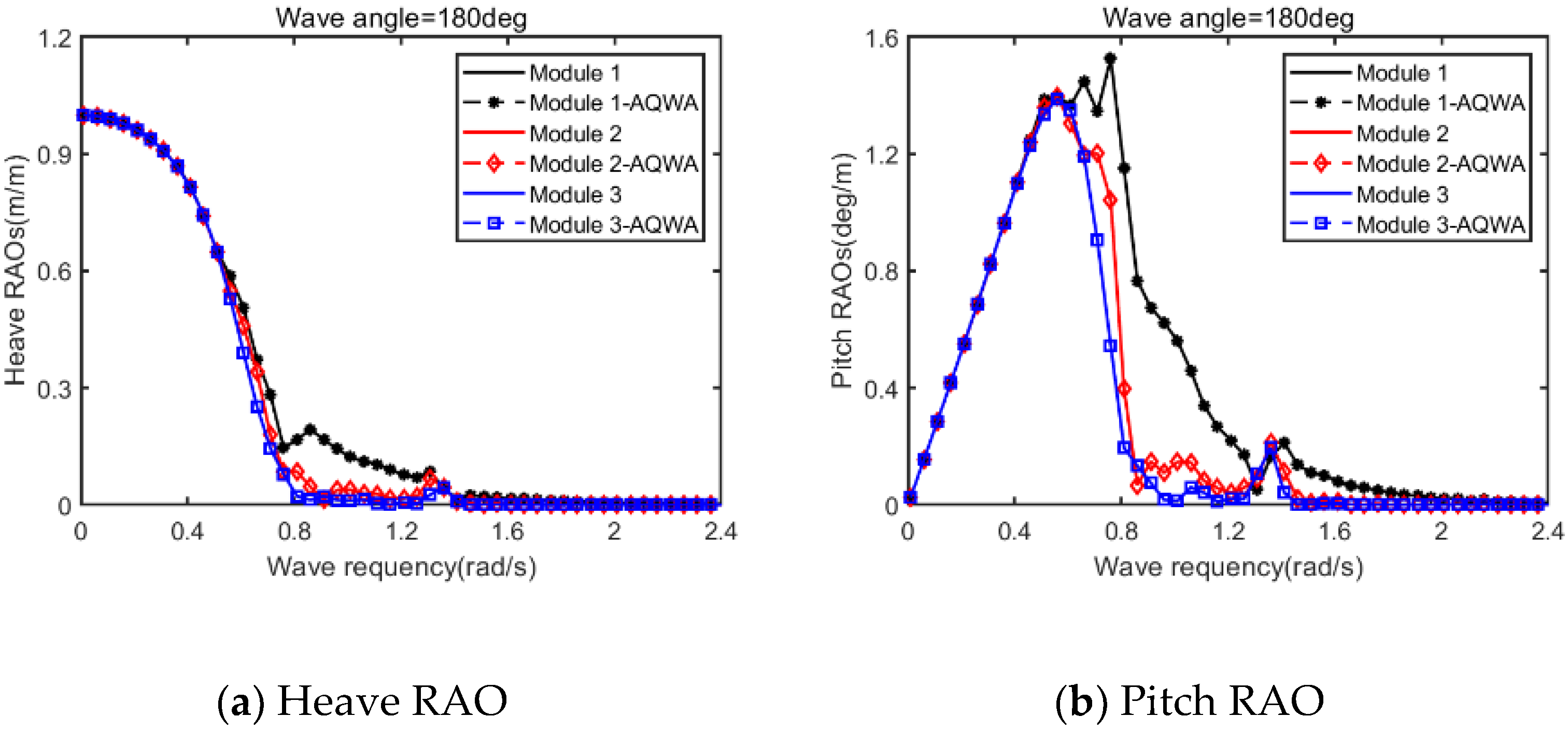
After introducing the damping lid factor, the hydrodynamic coefficients calculated by ANSYS-AQWA can be further input into the coupled CPHSTDM for post-processing and analysis. The frequency-domain RAOs of the three-module system in free-floating conditions by solving Equation (10) are first compared with the ones obtained by ANSYS-AQWA to verify the accuracy of the developed program. Figure 7 shows the comparisons of the surge, heave, and pitch RAOs of three different modules of the three-module system in a free-floating state with a gap width of 5 m under the head sea. It can be observed that the motion responses obtained by two different computational tools are highly consistent, which verifies that the hydrodynamic coefficients to be used in the CPHSTDM, i.e., wave force, added mass, and additional damping, are the same as those used in ANSYS-AQWA.

Based on the free-floating model in the frequency domain, the stiffness and mass attributes of the connecting components are introduced into the equation of motion in the frequency domain using an additional matrix, and the three-module floating system under the constraint of the connector is now considered. A type of connector consisting of two beams joined end to end was used, which is illustrated schematically in Figure 4. The tensile rigidity, bending rigidity, and mass characteristics of the connector can be considered simultaneously due to the introduction of the concept of the Euler–Bernoulli beam. By solving Equation (11), the frequency-domain responses of the modules at any wave frequency can be obtained, and the effects of the stiffness of the connections can be analyzed. Heave and pitch responses of three modules under flexible connection constraints are plotted in Figure 8. Axial stiffness EA and mass per unit length of the connector are set to 1.0 × 10¹⁰ N and 10 kg/m, respectively, and the kinematic characteristics of the system with different bending stiffness EI are to be discussed. There is no restoring force in the surge direction considered in CPHSTDM by now, whether from mooring force or hydrostatic force. To remain consistent with the following time-domain analysis, axial stiffness EA is set to be a constant. As for the mass of the connector, it should be noted that the mass of the connected component, consisting of four Euler–Bernoulli beams, accounts for a very small proportion of the total mass of the system, therefore the response to the change can also be ignored. Moreover, the stiffness of the connection joint C is selected as the same value as bending stiffness.

As illustrated in Figure 8, it can be seen that the bending stiffness of the connector would significantly affect the motion of the module, especially at low frequency, within 1 rad/s. Moreover, when EI is relatively small, the responses of each module exhibit behavior similar to those under free-floating conditions. It can be observed that the influence on the maximum pitch of the module is neglectable when EI is less than or equal to the order of 1.0 × 10⁹ Nm². With the increase in the bending stiffness, the differences between different modules decreased, because the overall system is more rigid due to the strengthening of the constraint effect. In addition, it should be noted that both the heave and pitch motions of Module 2 showed an obvious trend of weakening around 0.5 rad/s, while this phenomenon did not occur in Module 1 and Module 3. This is because it was in the center of the system and received the connection constraints from both the front and back sides. However, when the bending stiffness EI changes from 1.0 × 10⁶ Nm² to 1.0 × 10⁷ Nm², it has almost no effect on the heave motion of the floating body, and only has a slight change in the pitch motion at some frequencies.

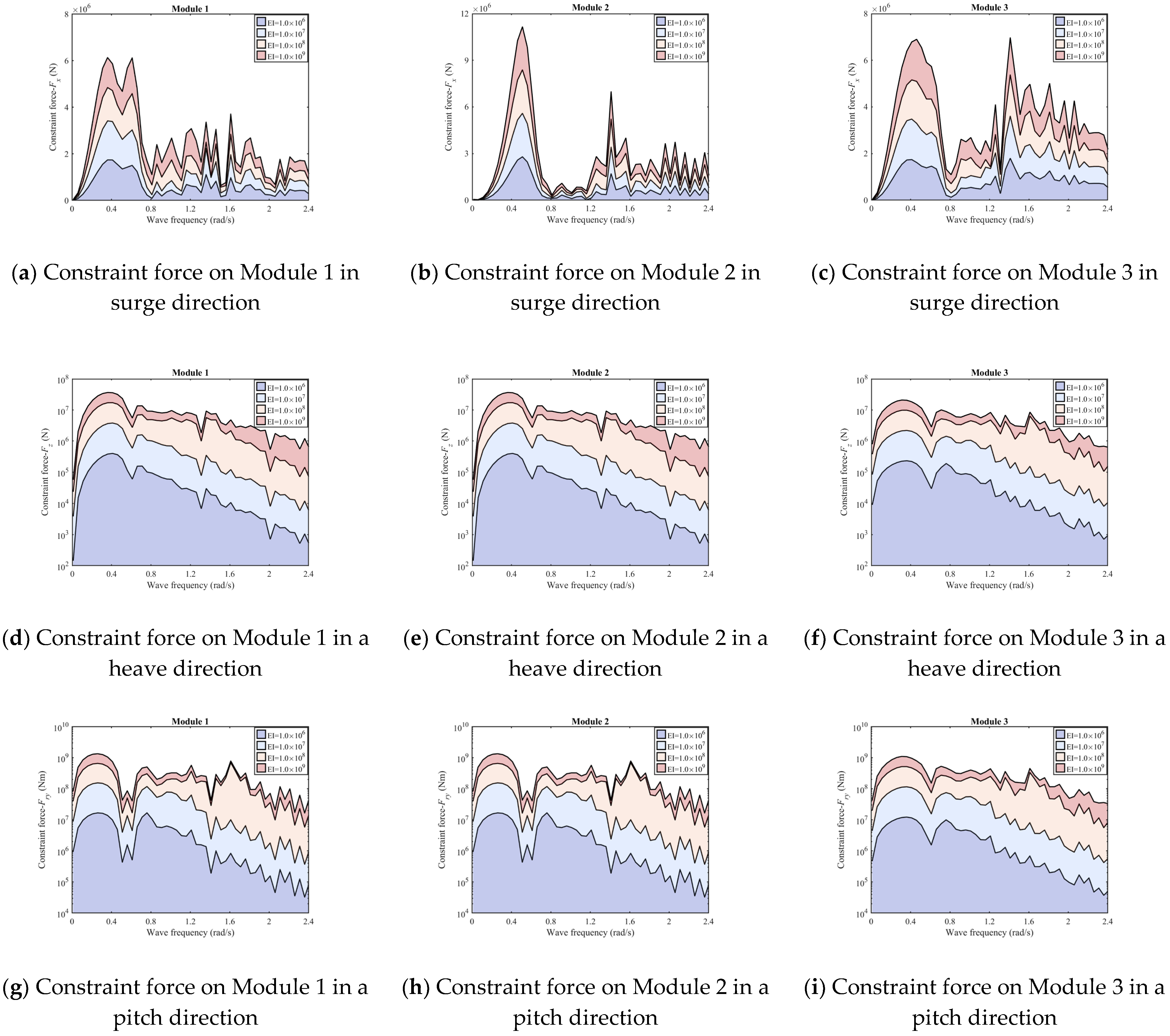
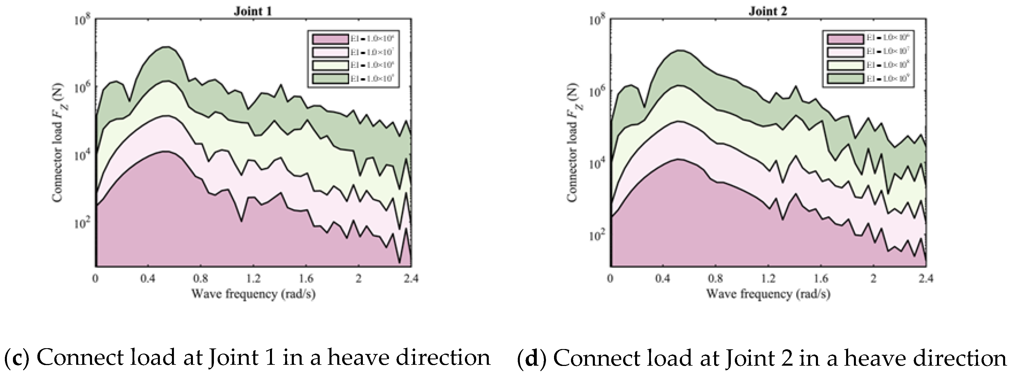
In addition to the frequency-domain responses, as one of the most important characteristics of the RMFC model, the constraint forces of the interconnected structure and loads of the connector itself caused by the relative motions of the adjacent modules are of vital importance for connector design in both academic research and engineering practice. Some typical results are given in Figure 9, showing the absolute values of the constraint forces on each module, respectively, plotted against wave frequency in the mode of surge, heave, and pitch. The peak value of the constraint force acting on each module are summarized in

Table 2. The peak value of the constraint force acting on each module.

Type	Bending Stiffness of the Connector	On Module 1	On Module 2	On Module 3
Fx	EI = 1.0 × 106 Nm2	1.74 × 106 N	2.80 × 106 N	1.80 × 106 N
	EI = 1.0 × 107 Nm2	1.67 × 106 N	2.80 × 106 N	1.74 × 106 N
	EI = 1.0 × 108 Nm2	1.56 × 106 N	2.80 × 106 N	1.80 × 106 N
	EI = 1.0 × 109 Nm2	1.53 × 106 N	2.77 × 106 N	1.80 × 106 N
Fz	EI = 1.0 × 106 Nm2	2.33 × 105 N	4.03 × 105 N	2.34 × 105 N
	EI = 1.0 × 107 Nm2	1.97 × 106 N	3.42 × 106 N	1.97 × 106 N
	EI = 1.0 × 108 Nm2	7.80 × 106 N	1.35 × 107 N	7.70 × 106 N
	EI = 1.0 × 109 Nm2	1.11 × 107 N	1.94 × 107 N	1.11 × 107 N
Mry	EI = 1.0 × 106 Nm2	1.22 × 107 Nm	1.69 × 107 Nm	1.22 × 107 Nm
	EI = 1.0 × 107 Nm2	1.03 × 108 Nm	1.39 × 108 Nm	1.04 × 108 Nm
	EI = 1.0 × 108 Nm2	4.09 × 108 Nm	5.02 × 108 Nm	4.04 × 108 Nm
	EI = 1.0 × 109 Nm2	5.82 × 108 Nm	6.80 × 108 Nm	5.82 × 108 Nm

. As the bending stiffness EI of the connector increases, the constraints imposed on each floating module become progressively more severe. The heave and pitch modes experience increasing constraint forces as the bending stiffness increases, although the rate of increase slows down. On the other hand, changes in stiffness barely affect the constraint forces in the surge direction. Figure 10 presents the effects of stiffness on the connector load and the peak value of the connector loads on common joints are summarized in

Table 3. The peak value of the connector loads on common joints.

Type	Bending Stiffness of the Connector	At Joint 1	At Joint 2
Fx	1.0 × 106 Nm2	36.9 N	36.9 N
	1.0 × 107 Nm2	36.9 N	36.9 N
	1.0 × 108 Nm2	36.8 N	36.8 N
	1.0 × 109 Nm2	36.5 N	36.5 N
Fz	1.0 × 106 Nm2	1.20 × 104 N	1.23 × 104 N
	1.0 × 107 Nm2	1.24 × 105 N	1.27 × 105 N
	1.0 × 108 Nm2	1.31 × 106 N	1.24 × 106 N
	1.0 × 109 Nm2	1.32 × 107 N	1.16 × 107 N

. As expected, the load at the common joint increases with stiffness. Notably, the force in the surge direction on the connector is significantly lower than that on the floating body. Nevertheless, the connector bears a larger load which is roughly similar to the load on the floating body in the heave motion.

3.3. Discussion of the Development of CPHSTDM and Parametric Study on Connector Parameters

After obtaining the hydrodynamic coefficients in the frequency domain, one can establish a time-domain model based on the Cummins equation. By replacing the convolution terms in the Cummins equation with state–space models (SSMs) and further considering the constraints between modules, the constant-parameter hydrodynamic–structural time-domain model (CPHSTDM) is then developed.

Since the multi-module floating system would experience strong hydrodynamic interactions, the damping lid method is employed to obtain reasonable hydrodynamic coefficients. The damping lid introduced in the multi-floating system not only affects the attenuation efficiency of the impulse response function [1], but also affects the accuracy of the constructed SSM, which has been verified by Zou et al. [6]. In this study, the frequency-domain results with damping lid factor α = 0.1 are used to develop the time-domain model. As the key step in CPHSTDM, appropriate parametric matrices of SSMs obtained via system identification based on the calculated impulse response function can be vital for the subsequent time-domain analysis. The established SSMs are quantified by the value of R² defined in Equation (31), where the value of 0.97 for R² is proved by Duarte et al. [52] to be sufficient to satisfy the time-domain accuracy in the single floating system.

Figure 11 shows that excellent fitting quality of the MDOF SSMs for the calculated K(t) of the windward module is achieved when the order of the SSMs is selected to be 40.

In addition, the corresponding R² of the SSMs for the coupled terms between different modules in the selected motions are summarized in

Table 4. R² values for SSMs identified based on the frequency-domain results for the coupling term between different modules.

k-SSM	R2 Defined by Equation (31)
40	K1,13(t)	K3,15(t)	K5,17(t)
	0.99568	0.99957	0.99286
	K1,7(t)	K3,9(t)	K5,11(t)
	0.9986	0.99905	0.99862
	K7,13(t)	K9,15(t)	K11,17(t)
	0.9986	0.99903	0.9984

. The R² values of the system shown in Figure 11 and Table 4 are greater than 0.99, surpassing the suggested value of 0.97 by Duarte et al. [56].

In this study, surge, heave, and pitch are the only modes of interest when the system is subjected to head sea. Based on the identified SSMs, the coupled nine-DOF time-domain model is established, which can take the constraint effect of the connectors into account. To analyze the three-module interconnected system under the head sea, the stiffness and mass matrix of the connecting system obtained in the frequency domain also play fundamental roles in the CPHSTDM. By solving Equation (30), the time-domain dynamic response of each module subjected to specified incident waves can be obtained, in which the fourth-order Runge–Kutta (RK4) integration method is used to solve the Cummins equation with a time step of 0.1 s. The numerical simulation costs about 100 s for a simulation duration of 500 s (AMD Ryzen™ 7 2700 Eight-Core Processor 3.20 GHz).

The application of the substructure method based on the static condensation in a floating-body system makes the CPHSTDM by Equation (30) equivalent to the frequency-domain model by Equation (11) in a free-floating state. Therefore, the widely used method of frequency–time-domain verification in free floating can be used for reference, i.e., the accuracy of time-domain model calculation can be estimated by comparing the time-domain results with the corresponding frequency-domain RAOs.

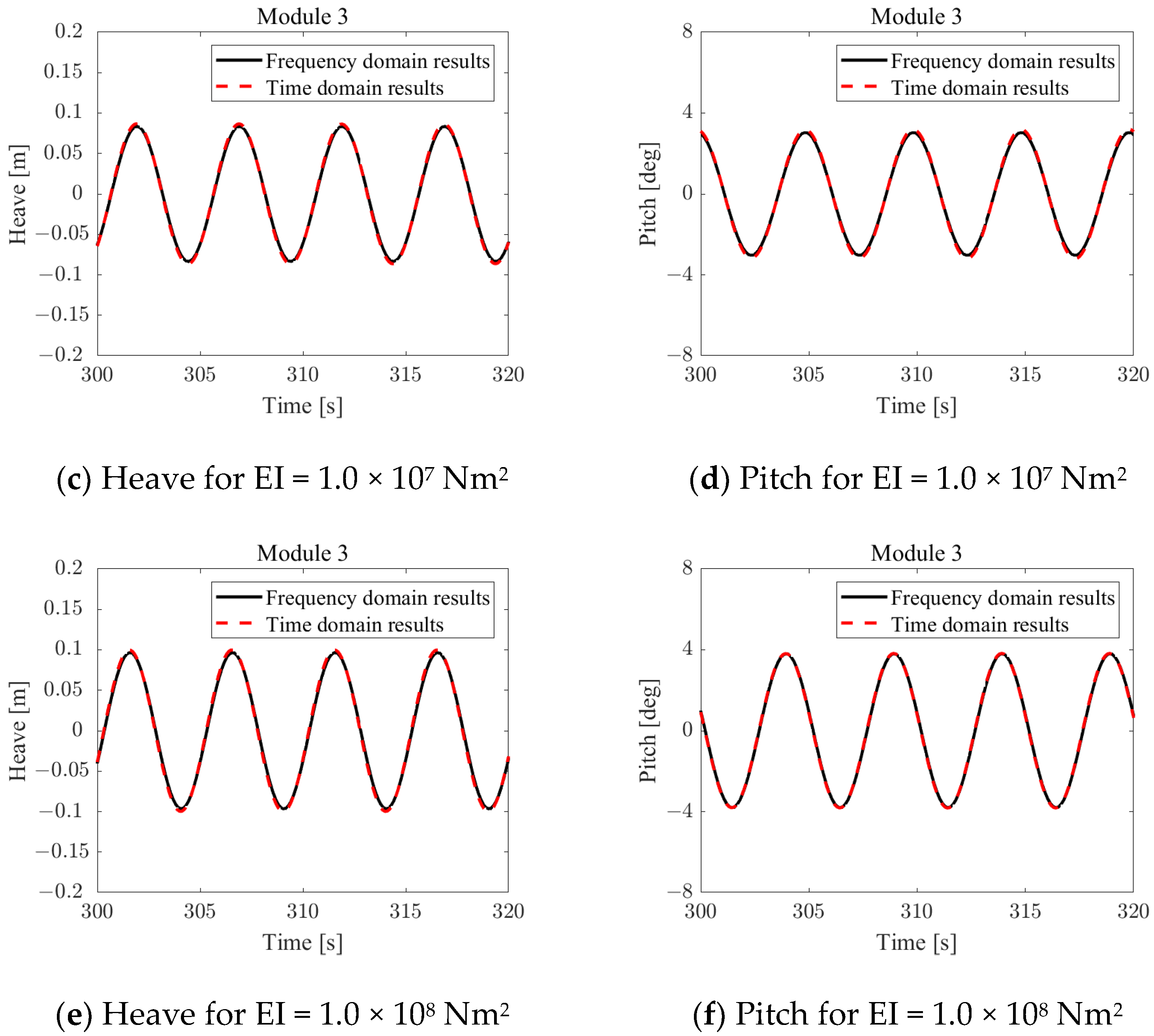
Figure 12 shows a comparison between the RAO-based response and the results of the CPHSTDM for the heave and pitch motions of the windward module. Several connector stiffness values are considered in this comparison. The wave amplitude is 2 m, and the wave frequency is 1.26 rad/s, which is close to the frequency at which hydrodynamic resonance occurs. The results of the CPHSTDM show high accuracy compared to the RAO-based responses, which indicates that the time-domain results are reliable and can be used for further analysis. However, it should be noted that the connector stiffness EI is 1.0 × 10⁹ Nm², and a resonance phenomenon occurs, making it impossible to obtain stable time-domain results. This phenomenon may have something to do with the hydrostatic restoring force in pitch–pitch mode, with the pitch–pitch stiffness being 4.1732 × 10¹⁰ Nm/rad. Therefore, for the time-domain comparison, the value of EI equal to 1.0 × 10⁹ Nm², is not considered.

Due to the constraint effect of connectors between adjacent modules, the three floating bodies form a whole in the mode of the surge and the motion response of each unit module is consistent. Therefore, only the heave and pitch motions of each module are plotted here to reveal the influence of different connector parameters on the dynamic characteristics of the whole system. The connector between the two beam units is semi-rigid, and therefore, the overall pitch response results demonstrate uniformity for different bending stiffness EI values, in the order of 10⁻³. However, it is crucial to note that the motion amplitude of each module is not necessarily the same. On the other hand, it can also be seen that the heave response amplitude of the floating system under various connection stiffness is different, but there is no significant difference between the results when the stiffness EI is 1.0 × 10⁶ Nm² and 1.0 × 10⁷ Nm², which remain consistent with the conclusion drawn in the frequency-domain model.

The periodic response characteristics can be illustrated from regular wave analysis in CPHSTDM. Figure 13 demonstrates the comparison of the heave motions of the three modules under a regular wave of ω = 1.26 rad/s and wave amplitude of 2 m in the head sea for different connector stiffness. The typical time is chosen when the windward module is at the peak of its own heave motion, which is shown in the right image of the figure with the colors of the modules corresponding to their own motion curves in the left. The areas in slash shadow are the wet surfaces of the modules under calm water while those in dotted shadow are the dry surfaces. The results clearly show the position relationship between the three modules in the system.

With the value of EI increasing from 1.0 × 10⁶ Nm² to 1.0 × 10⁷ Nm², the phases of the responses of all three modules are hardly affected. However, when the EI is set to 1.0 × 10⁸ Nm², the response amplitudes of Module 2 and Module 3 exhibit differing extents of increase compared to the former two cases. Notably, the response amplitude of Module 1 experiences a slight decrease. No phase shift occurs on the responses of both Module 2 and Module 3, while Module 1 seems to have a positive phase shift when the value of EI is set to 1.0 × 10⁸ Nm², which indicates that the heave response of Module 1 lags more compared to the previous cases.

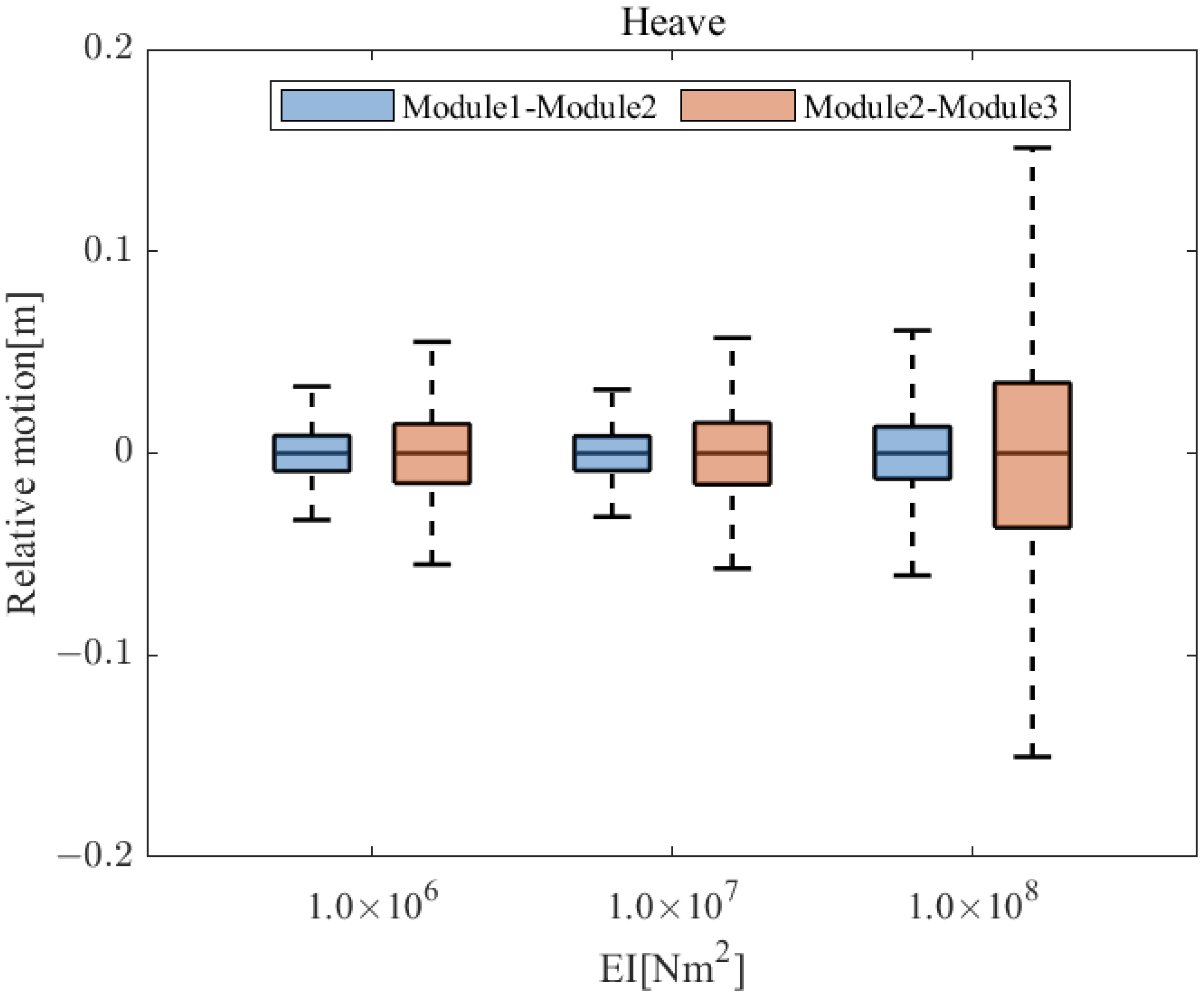
In addition to the individual motions of each floating body, the relative motion between adjacent modules is also an important concern in multi-floating system application scenarios, such as a floating airport. According to the time-domain results obtained by the CPHSTDM, a box plot is demonstrated to reveal the statistics of the relative heave motion of adjacent modules under different connector parameters in Figure 14. Due to the shielding effect, the relative heave motion between the two leeward bodies, Module 1 and Module 2 is weaker than that of the two windward bodies, Module 2 and Module 3. Moreover, when the bending stiffness is set to 1.0 × 10⁸ Nm², the relative motion between Module 2 and Module 3 is significantly greater than those when the value of EI is lower.

4. Concluding Remarks

A coupled constant-parameter hydrodynamic–structural model (CPHTDM) has been established in this study, which can be used to investigate the dynamics of a multi-module floating system with flexible connectors between adjacent floating bodies. A three-module floating system, which has been studied in the previous study, is further analyzed after increasing the gap width to 5 m using the standard panel code AQWA. With the employment of the dynamic substructure method, structural parameters such as stiffness and mass of flexible connectors can be fully considered and equipped in the whole system, which provides a basis for the analysis of the interconnected multi-module floating system in both the frequency domain and time domain. In this study, the frequency-domain model, which has been verified by published papers [5,49,50,58], is further extended to the time domain, and the behaviors of the system are investigated by the developed CPHSTDM. Considering that strong hydrodynamic interactions are a severe problem in the multi-module floating system in which the floating bodies operate with a small gap between each other, the external damping lid method is applied to ensure the precision of the analysis in AQWA. On this basis, the modified frequency-domain results with viscosity correction are transformed into the time domain using the Ogilvie relationship, and the Cummins equation is further used to construct the CPHSTDM, in which the SSM is used to replace the time-consuming convolution term. After finishing the construction of the CPHSTDM, the time-domain response is further demonstrated. Some findings can be confirmed from this investigation.

• The effects of hydrodynamic interactions in the multi-module floating system play a crucial role in the response of the system and directly affect the feasibility of the numerical model calculation, especially when transforming the frequency-domain results into the time domain. When the distorted hydrodynamic interaction results in potential theory are corrected, it would lead to stable time-domain results.
• Connector parameters such as bending stiffness have a significant impact on overall system performance. Both the response of the floating body and the internal load such as forces and moments obtained through the connections between adjacent modules are affected to varying degrees. For the semi-rigid connection system analyzed here, since the tension–compression characteristics are mainly determined by the axial stiffness EA, the force along the connector layout shows signs of insensitivity to different bending stiffness EI. With the exponential increase of the bending stiffness, loads in the surge direction seem to be insensitive for both connectors and the joint, while the loads in the heave and pitch direction of the connectors exhibit first exponential growth and then a slow-down at EI = 1.0 × 10⁹ Nm².
• The development of CPHSTDM makes it possible not only to analyze the system behaviors such as the specific motion state at a certain time and the relative motion between adjacent modules under the connection constraints, but also to judge the influence of stiffness selection on the whole system so that the phenomenon of global resonance caused by inappropriate stiffness selection can be avoided in the analysis of practical problems.

In addition to analyzing the three-module floating system aligned in series, the developed numerical model can be extended to N floating bodies provided that the hardware performance is not limited. Meanwhile, the application of the CPHSTDM provides the probability to analyze complex connector configurations. For example, connectors with bending stiffness or hyperstatic marine systems are not available in AQWA, but it is possible by employing the Euler–Bernoulli beam in the CPHSTDM. Therefore, the CPHSTDM is suitable for analyzing complex and flexible connections, which makes the model more applicable to various marine operation scenarios, such as float-over installation and wave energy converters. The use of the RMFC model can be expanded to other scenarios with CPHSTDM.

It should be noted that the coupled numerical model developed in this study only considers the linear wave excitation forces and only regular waves are considered in the time-domain simulation. However, according to the previous works on the SSM [4,6,7,43,46,59], it is recommended to extend the analysis into irregular wave scenarios, and second-order wave forces on the mooring model, such as MoorDyn [60], can be further introduced to complete the whole system’s nonlinear dynamic characteristics of the mooring state in the future study. Moreover, it is a limitation that the Euler–Bernoulli beam model used in this study is based on the vertical planar motion assumptions. The 6-DOF response of each module in an environment such as oblique waves cannot be accurately captured by the present model considering only the coupled surge–heave–pitch motions. Hence, future studies are recommended to use the space flexible beam model to achieve full DOF simulation, and therefore many marine operation problems involving complex wave conditions, such as the floating breakwater and floating bridge, can be analyzed in the time domain based on the developed CPHSTDM. In addition, the developed CPHSTDM can also be applied to other configurations, e.g., the floating photovoltaic system as analyzed by Li and Choung [61].

References

- Chen, M.; Guo, H.; Wang, R.; Tao, R.; Cheng, N. Effects of gap resonance on the hydrodynamics and dynamics of a multi-module floating system with narrow gaps. J. Mar. Sci. Eng. 2021, 9, 1256. [Google Scholar] [CrossRef]
- Koo, B.J.; Kim, M.H. Hydrodynamic interactions and relative motions of two floating platforms with mooring lines in side-by-side offloading operation. Appl. Ocean Res. 2005, 27, 292–310. [Google Scholar] [CrossRef]
- Zhao, W.; Yang, J.; Hu, Z.; Tao, L. Prediction of hydrodynamic performance of an FLNG system in side-by-side offloading operation. J. Fluids Struct. 2014, 46, 89–110. [Google Scholar] [CrossRef]
- Chen, M.; Eatock Taylor, R.; Choo, Y.S. Time domain modelling of the wave induced dynamics of multiple structures in close proximity. In Proceedings of the 3rd Marine Operations Specialty Symposium (MOSS), Singapore, 20–21 September 2016. [Google Scholar]
- Chen, M.; Zou, M.; Zhu, L. Frequency-domain response analysis of adjacent multiple floaters with flexible connections. J. Ship Mech. 2018, 22, 1164–1180. [Google Scholar]
- Zou, M.; Chen, M.; Zhu, L.; Li, L.; Zhao, W. A constant parameter time domain model for dynamic modelling of multi-body system with strong hydrodynamic interactions. Ocean. Eng. 2023, 268, 113376. [Google Scholar] [CrossRef]
- Chen, M.; Xiao, P.; Zhou, H.; Li, C.B.; Zhang, X. Fully Coupled Analysis of an Integrated Floating Wind-Wave Power Generation Platform in Operational Sea-States. Front. Energy Res. 2022, 10, 931057. [Google Scholar] [CrossRef]
- Zhang, X.; Li, B.; Hu, Z.; Deng, J.; Xiao, P.; Chen, M. Research on size optimization of wave energy converters based on a floating wind-wave combined power generation platform. Energies 2022, 15, 8681. [Google Scholar] [CrossRef]
- McAllister, K.R. Mobile offshore bases—An overview of recent research. J. Mar. Sci. Technol. 1997, 2, 173–181. [Google Scholar] [CrossRef]
- Remmers, G.; Zueck, R.; Palo, P.; Taylor, R. Mobile offshore base. In Proceedings of the The Eighth International Offshore and Polar Engineering Conference, Montréal, QC, Canada, 24–29 May 1998. [Google Scholar]
- Sakthivel, S.; Kumar, N.; Poguluri, S.K. Dynamic responses of serially connected truss pontoon-MOB—A numerical investigation. Ocean Eng. 2023, 277, 114209. [Google Scholar] [CrossRef]
- Jin, J. A Mixed Mode Function-Boundary Element Method for Very Large Floating Structure-Water Interaction Systems Excited by Airplane Landing Impacts. Ph.D. Thesis, University of Southampton, Southampton, UK, 2007. [Google Scholar]
- Fu, S.; Moan, T.; Chen, X.; Cui, W. Hydroelastic analysis of flexible floating interconnected structures. Ocean Eng. 2007, 34, 1516–1531. [Google Scholar] [CrossRef]
- Gao, R.; Wang, C.; Koh, C. Reducing hydroelastic response of pontoon-type very large floating structures using flexible connector and gill cells. Eng. Struct. 2013, 52, 372–383. [Google Scholar]
- Gao, J.-l.; Lyu, J.; Wang, J.-H.; Zhang, J.; Liu, Q.; Zang, J.; Zou, T. Study on Transient Gap Resonance with Consideration of the Motion of Floating Body. China Ocean Eng. 2022, 36, 994–1006. [Google Scholar] [CrossRef]
- Gao, J.; Gong, S.; He, Z.; Shi, H.; Zang, J.; Zou, T.; Bai, X. Study on Wave Loads during Steady-State Gap Resonance with Free Heave Motion of Floating Structure. J. Mar. Sci. Eng. 2023, 11, 448. [Google Scholar] [CrossRef]
- Molin, B. On the piston and sloshing modes in moonpools. J. Fluid Mech. 2001, 430, 27–50. [Google Scholar] [CrossRef]
- Zhao, W.; Pan, Z.; Lin, F.; Li, B.; Taylor, P.H.; Efthymiou, M. Estimation of gap resonance relevant to side-by-side offloading. Ocean Eng. 2018, 153, 1–9. [Google Scholar] [CrossRef]
- Jiang, D.; Tan, K.H.; Wang, C.M.; Dai, J. Research and development in connector systems for very large floating structures. Ocean Eng. 2021, 232, 109150. [Google Scholar] [CrossRef]
- Riggs, H.; Ertekin, R.; Mills, T. Impact of stiffness on the response of a multimodule mobile offshore base. Int. J. Offshore Polar Eng. 1999, 9, 126–133. [Google Scholar]
- Haney, J. Mob connector development. In Proceedings of the 3rd International Workshop on Very Large Floating Structures, Honolulu, HI, USA, 22–24 September 1999; Ertekin, R.C., Ed.; School of Ocean & Earth Science & Technology: Honolulu, HI, USA, 1999. VLFS’99. Volume 2. [Google Scholar]
- Rognaas, G.; Xu, J.; Lindseth, S.; Rosendahl, F. Mobile offshore base concepts. Concrete hull and steel topsides. Mar. Struct. 2001, 14, 5–23. [Google Scholar] [CrossRef]
- Xu, D.; Zhang, H.; Qi, E.; Hu, J.; Wu, Y. On study of nonlinear network dynamics of flexibly connected multi-module very large floating structures. In Vulnerability, Uncertainty, and Risk: Quantification, Mitigation, and Management, Proceedings of the Second International Conference on Vulnerability and Risk Analysis and Management (ICVRAM) and the Sixth International Symposium on Uncertainty Modeling and Analysis (ISUMA), Liverpool, UK, 13–16 July 2014; American Society of Civil Engineers: Reston, VA, USA, 30 October 2014; pp. 1805–1814. [Google Scholar]
- Wu, L.; Wang, Y.; Xiao, Z.; Li, Y. Hydrodynamic response for flexible connectors of mobile offshore base at rough sea states. Pet. Explor. Dev. 2016, 43, 1089–1096. [Google Scholar] [CrossRef]
- Xia, D.; Kim, J.W.; Ertekin, R.C. On the hydroelastic behavior of two-dimensional articulated plates. Mar. Struct. 2000, 13, 261–278. [Google Scholar] [CrossRef]
- Zhao, H.; Xu, D.; Zhang, H.; Shi, Q. A flexible connector design for multi-modular floating structures. In Proceedings of the International Conference on Offshore Mechanics and Arctic Engineering, Madrid, Spain, 17–22 June 2018; p. V001T001A018. [Google Scholar]
- Qi, E.; Liu, C.; Xia, J.; Lu, Y.; Li, Z.; Yue, Y. Experimental study of functional simulation for flexible connectors of very large floating structures. J. Ship Mech. 2015, 19, 1245–1254. [Google Scholar]
- Zhang, H.; Qi, E.R.; Song, H.; Li, Z.W.; Xia, J.S. Study on mechanical property of connector with flexible sandwich of very large floating structures. J. Ship Mech. 2019, 23, 200–210. [Google Scholar]
- Loukogeorgaki, E.; Lentsiou, E.N.; Aksel, M.; Yagci, O. Experimental investigation of the hydroelastic and the structural response of a moored pontoon-type modular floating breakwater with flexible connectors. Coast. Eng. 2017, 121, 240–254. [Google Scholar] [CrossRef]
- Ding, J.; Wu, Y.-S.; Zhou, Y.; Ma, X.-Z.; Ling, H.J.; Xie, Z. Investigation of connector loads of a 3-module VLFS using experimental and numerical methods. Ocean Eng. 2020, 195, 106684. [Google Scholar] [CrossRef]
- Michailides, C.; Loukogeorgaki, E.; Angelides, D.C. Response analysis and optimum configuration of a modular floating structure with flexible connectors. Appl. Ocean Res. 2013, 43, 112–130. [Google Scholar] [CrossRef]
- Yang, P.; Li, Z.; Wu, Y.; Wen, W.; Ding, J.; Zhang, Z. Boussinesq-Hydroelasticity coupled model to investigate hydroelastic responses and connector loads of an eight-module VLFS near islands in time domain. Ocean Eng. 2019, 190, 106418. [Google Scholar] [CrossRef]
- Bispo, I.B.S.; Mohapatra, S.C.; Guedes Soares, C. Numerical model of a WEC-type attachment of a moored submerged horizontal set of articulated plates. Trends Marit. Technol. Eng. 2022, 2, 335–344. [Google Scholar]
- Bispo, I.B.S.; Mohapatra, S.C.; Guedes Soares, C. Numerical analysis of a moored very large floating structure composed by a set of hinged plates. Ocean Eng. 2022, 253, 110785. [Google Scholar] [CrossRef]
- Cummins, W. The impulse response function and ship motions. Schiffstechnik 1962, 9, 101–109. [Google Scholar]
- Tian, W.; Wang, Y.; Shi, W.; Michailides, C.; Wan, L.; Chen, M. Numerical study of hydrodynamic responses for a combined concept of semisubmersible wind turbine and different layouts of a wave energy converter. Ocean Eng. 2023, 272, 113824. [Google Scholar] [CrossRef]
- Shi, W.; Li, J.; Michailides, C.; Chen, M.; Wang, S.; Li, X. Dynamic Load Effects and Power Performance of an Integrated Wind–Wave Energy System Utilizing an Optimum Torus Wave Energy Converter. J. Mar. Sci. Eng. 2022, 10, 1985. [Google Scholar] [CrossRef]
- Chen, M.; Yuan, G.; Li, C.B.; Zhang, X.; Li, L. Dynamic analysis and extreme response evaluation of lifting operation of the offshore wind turbine jacket foundation using a floating crane vessel. J. Mar. Sci. Eng. 2022, 10, 2023. [Google Scholar] [CrossRef]
- Wang, D.; Ertekin, R.C.; Riggs, H.R. Three-dimensional hydroelastic response of a very large floating structure. Int. J. Offshore Polar Eng. 1991, 1, 307–316. [Google Scholar]
- Wang, Y.; Wang, X.; Xu, S.; Wang, L.; Ding, A.; Deng, Y. Experimental and Numerical Investigation of Influences of Connector Stiffness and Damping on Dynamics of a Multimodule VLFS. Int. J. Offshore Polar Eng. 2020, 30, 427–436. [Google Scholar] [CrossRef]
- Chen, M.; Zou, M.; Zhu, L.; Sun, L. Numerical analysis of GBS float-over deck installation at docking and undocking stages based on a coupled heave-roll-pitch impact model. In Proceedings of the ASME 2019 38th International Conference on Ocean, Offshore and Arctic Engineering, Glasgow, UK, 9–14 June 2019; American Society of Mechanical Engineers: New York, NY, USA, 2019. [Google Scholar]
- Chen, M.; Eatock Taylor, R.; Choo, Y.S. Time domain modeling of a dynamic impact oscillator under wave excitations. Ocean Eng. 2014, 76, 40–51. [Google Scholar] [CrossRef]
- Chen, M.; Eatock Taylor, R.; Choo, Y.S. Investigation of the complex dynamics of float-over deck installation based on a coupled heave-roll-pitch impact model. Ocean Eng. 2017, 137, 262–275. [Google Scholar] [CrossRef]
- Zou, M.; Zhu, L.; Chen, M. Numerical simulation of the complex impact behavior of float-over deck installation based on an efficient two-body heaving impact model. In Proceedings of the ASME 2018 37th International Conference on Ocean, Offshore and Arctic Engineering, Madrid, Spain, 17–22 June 2018; American Society of Mechanical Engineers: New York, NY, USA, 2018. [Google Scholar]
- Zhu, L.; Zou, M.; Chen, M.; Li, L. Nonlinear dynamic analysis of float-over deck installation for a GBS platform based on a constant parameter time domain model. Ocean Eng. 2021, 235, 109443. [Google Scholar] [CrossRef]
- Chen, M.; Xiao, P.; Zhang, Z.; Sun, L.; Li, F. Effects of the end-stop mechanism on the nonlinear dynamics and power generation of a point absorber in regular waves. Ocean Eng. 2021, 242, 110123. [Google Scholar] [CrossRef]
- Hsu, C.S. On dynamic stability of elastic bodies with prescribed initial conditions. Int. J. Eng. Sci. 1966, 4, 1–21. [Google Scholar] [CrossRef]
- Liu, H.; Chen, M.; Han, Z.; Zhou, H.; Li, L. Feasibility study of a novel open ocean aquaculture ship integrating with a wind turbine and an internal turret mooring system. J. Mar. Sci. Eng. 2022, 10, 1729. [Google Scholar] [CrossRef]
- Sun, L.; Choo, Y.S.; Eatock Taylor, R.; Llorente, C. Responses of floating bodies with flexible connections. In Proceedings of the 2nd Marine Operations Specialty Symposium, Singapore, 6–8 August 2012; pp. 229–243. [Google Scholar]
- Eatock Taylor, R.; Taylor, P.; Stansby, P. A coupled hydrodynamic–structural model of the M4 wave energy converter. J. Fluids Struct. 2016, 63, 77–96. [Google Scholar] [CrossRef]
- Sun, L.; Eatock Taylor, R.; Choo, Y.S. Responses of interconnected floating bodies. IES J. Part A Civ. Struct. Eng. 2011, 4, 143–156. [Google Scholar] [CrossRef]
- Przemieniecki, J.S. Theory of Matrix Structural Analysis; Courier Corporation: Chelmsford, MA, USA, 1985. [Google Scholar]
- Qu, Z.-Q. Model Order Reduction Techniques with Applications in Finite Element Analysis: With Applications in Finite Element Analysis; Springer Science & Business Media: Berlin, Germany, 2004. [Google Scholar]
- Ogilvie, T.F. Recent Progress Towards the Understanding and Prediction of Ship Motions. In Proceedings of the Sixth Symposium on Naval Hydrodynamics, Washington, DC, USA, 28 September–4 October 1966. [Google Scholar]
- Taghipour, R.; Perez, T.; Moan, T. Hybrid frequency–time domain models for dynamic response analysis of marine structures. Ocean Eng. 2008, 35, 685–705. [Google Scholar] [CrossRef]
- Duarte, T.; Sarmento, A.; Alves, M.; Jonkman, J. State-Space Realization of the Wave-Radiation Force within FAST. In Proceedings of the 32nd International Conference on Ocean, Offshore and Arctic Engineering, Nantes, France, 9–14 June 2013. [Google Scholar]
- Cheetham, P.; Du, S.; May, R.; Smith, S. Hydrodynamic analysis of ships side by side in waves. In Proceedings of the International Aerospace CFD Conference, Paris, France, 25–28 June 2007. [Google Scholar]
- Sun, L.; Taylor, R.E.; Choo, Y.S. Multi-body dynamic analysis of float-over installations. Ocean Eng. 2012, 51, 1–15. [Google Scholar] [CrossRef]
- Hu, Z.; Li, X.; Zhao, W.; Wu, X. Nonlinear dynamics and impact load in float-over installation. Appl. Ocean Res. 2017, 65, 60–78. [Google Scholar] [CrossRef]
- Hall, M. MoorDyn User’s Guide; Department of Mechanical Engineering, University of Maine: Orono, ME, USA, 2015. [Google Scholar]
- Li, C.B.; Choung, J. Structural Effects of Mass Distributions in a Floating Photovoltaic Power Plant. J. Mar. Sci. Eng. 2022, 10, 1738. [Google Scholar] [CrossRef]
Figure 1.
Dynamic model with flexible substructures.
Figure 2.
Diagram of horizontal beam connector.
Figure 3.
Notation of the three-module hydrodynamic–structural model.
Figure 4.
Plan view of the system and connector modeling.
Figure 5.
Comparison of the added mass coefficients.
Figure 6.
Comparison of the added damping coefficients.
Figure 7.
Comparison between the developed numerical model and the well-proven panel code AQWA.
Figure 8.
Heave and pitch motions of modules under different connection parameters.
Figure 9.
Constraint forces on each module under the action of connectors.
Figure 10.
Connector loads on common joints between beam elements.
Figure 11.
Fitting quality of the MDOF SSM for K(t) based on the frequency-domain results with damping lid factor α = 0.1.
Figure 12.
Comparisons of heave and pitch motions of Module 3 between the RAO-based response and CPHSTDM-based response under the regular wave of ω = 1.26 rad/s and wave amplitude of 2 m in the head sea for different connector stiffness.
Figure 13.
The system’s instantaneous motion state under different connector stiffness when the windward module’s heave motion is at the peak at ω = 1.26 rad/s and wave amplitude of 2 m in a head sea.
Figure 14.
Relative motion between adjacent modules in a heave direction with different connector stiffness.