
Impacts of Tidal Oscillations on Coastal Groundwater System in Reclaimed Land
by
 and
and
Jing Guo
1,
Ye Ma
1,2,*,
Chao Ding
3,
Huawen Zhao
4,
Zhixin Cheng
1,2,
Guanxi Yan
5 and
and
Zaijin You
2 1
College of Environmental Science and Engineering, Dalian Maritime University, Dalian 116026, China
2
Centre for Ports and Maritime Safety, Dalian Maritime University, Dalian 116000, China
3
Dalian Ecological Environment Affairs Service Center, Dalian 116000, China
4
Key Laboratory of Coastal Environment and Resources of Zhejiang Province, School of Engineering, Westlake University, Hangzhou 310030, China
5
School of Civil Engineering, University of Queensland, St. Lucia, Brisbane, QLD 4072, Australia
*
Author to whom correspondence should be addressed.
J. Mar. Sci. Eng. 2023, 11(10), 2019; https://doi.org/10.3390/jmse11102019
Submission received: 9 September 2023
/
Revised: 17 October 2023
/
Accepted: 18 October 2023
/
Published: 20 October 2023
(This article belongs to the Section Ocean Engineering)
Abstract
:The impact of tidal oscillations on groundwater in coastal reclamation land demonstrates the complex hydrodynamic interaction between seawater and coastal hydrological aquifer systems. The tidal action not only affects the temporal variability of groundwater levels but also exerts a significant influence on the groundwater gradients of salinity within the subsurface aquifers. This study takes the Songmu Area as an example to investigate this ocean–groundwater interaction. Songmu Area is located on a peninsula with coastal land reclamation in Dalian, China. Field campaigns were conducted in this area to measure the tidal action and groundwater parameters in a coastal reclaimed area at artificial backfill layers with pressure and salinity sensors, where the tidal signal can influence groundwater levels and salinity up to a one-kilometer range of inland. Tidal changes in the surface of the sea can be broken down into a number of simple, regular harmonic vibrations, each of which is called a tidal split. The tide and groundwater data were extracted using an enhanced harmonic analysis method. The fluctuations of groundwater levels and salinity were decomposed in response to the periodic tidal oscillation. Various constituents of tide attenuation in the coastal groundwater system were investigated. Our research shows that there is an exponential reduction in the fluctuating amplitude of groundwater levels and the groundwater salinity as distance further inland from the coast. The constituents of tide M2 (the period is 12.42 h of semi-diurnal tides, S2 (the period is 12.00 h of semi-diurnal tides), K1 (the period is 23.93 h of full-diurnal tides), and O1 (the period is 25.82 h of full-diurnal tides) behave differently for the tidal wave propagation and salinity variability in the coastal aquifer of reclaimed land. Among those constituents, M2 and S2 exhibit a higher degree of attenuation compared with K1 and O1. Understanding the relationship between groundwater levels and tidal fluctuations in coastal backfill areas is crucial for effective groundwater management strategies and mitigating the adverse impacts of seawater intrusion. This study can serve as a good understanding for assessing the impacts of various mitigation strategies.
1. Introduction
Studies on groundwater systems in the coastal zones under anthropogenic influence are of significance for the protection of the marine environment and the growth of the coastal economy. Dynamics in a coastal groundwater system have vital impacts on coastal water nutrients and pollution, water resource safety, and the geography evolution [1]. The fluctuation of the coastal groundwater table is influenced by various factors such as precipitation, evaporation, storm surge, water extraction, and tide [2]. The impact of the rainfall and evapotranspiration on the coastal groundwater system could be within the time frame of days to months. Our research primarily focuses on the ongoing reactions of the groundwater table to semi-diurnal and diurnal tidal variations. No storm surge was observed in the study area, so the impact of these conditions on the study area has not been considered. Furthermore, given the absence of pumping wells in the research region, the influence of pumping on groundwater was not considered. The sustained exploitation of coastal resources has not only damaged the ecological systems of these coastal regions but has also led to a range of environmental pollution issues in the marine environment [3]. Furthermore, oceanic dynamics, such as tidal action, can transport substances to neighboring groundwater systems, which can affect both regional and global pollutant exchange [4]. A better understanding of ocean–groundwater interaction in coastal areas, therefore, provides an important reference for management regarding coastal construction, aquaculture, industries, and tourism.
The coastal groundwater system within the industrial zone is characterized by relatively high permeability and the fast migration of solute; these dissolved matters have unique features that differ from those in inland groundwater: (1) they have a large range of varieties, and (2) their transport is strongly influenced by oceanic dynamics. These dissolved matters or pollutants are mainly from two sources: terrigenous matters discharged from industry activities and oceanic matters transported by tides or storms [5]. Terrestrial pollutant discharge into the nearshore areas is becoming an increasingly severe global issue [6]. Traditionally, river discharge was considered the primary source of marine chemical contaminants, while the direct discharge from groundwater has been a long-neglected critical factor. The oceanic source generally changes closely with the condition of tidal propagation. A significant number of field observations and numerical simulation studies have been conducted, highlighting the role of submarine groundwater discharge as an essential component of coastal aquifers in dominating the quantity of pollutant discharge into the sea [7]. Knowledge of the impacts of such oceanic processes on the groundwater system helps to understand the distribution and transport pattern of industry-oriented pollutants in coastal groundwater.
In natural conditions, seawater intrusion is a complex hydrogeological phenomenon driven by the density difference between seawater and freshwater. The occurrence of seawater intrusion depends upon various geological and hydrodynamic conditions. Geological conditions serve as the foundational pathways and movement of seawater intrusion. On the other hand, coastal hydrodynamic conditions act as the dominant controlling factors [8]. During the drought period, with the reduction in the hydraulic gradient, these dynamic variations alter the existing dynamic equilibrium between seawater and freshwater, thereby initiating severe seawater intrusion [9].
In addition, tidal action significantly influences groundwater levels, causing fluctuations that correspond with sea-level variations. A comprehensive analysis of how groundwater levels in sandy beach aquifers are affected by oceanic tidal actions has been conducted [10,11]. Furthermore, the variations in the water levels of confined aquifers due to oceanic tides were investigated to estimate their diffusion coefficients. In coastal aquifers, the groundwater level exhibits periodic fluctuations in response to tidal water level changes, a phenomenon known as the tidal effect [12]. This effect is particularly pronounced in coastal zones and has substantial implications for groundwater flow systems and pollutant migration pathways. Groundwater levels fluctuate due to tidal influences, exhibiting the same periodicity as tidal water levels but with a noticeably smaller amplitude and phase lag [13]. The extent of tidal influence varies significantly across different types of aquifers; for instance, confined aquifers are less affected by tidal actions compared to unconfined aquifers when evaluated under similar hydrogeological parameters [14]. Furthermore, periodic sea-level changes also prompt the redistribution of salt in coastal aquifers. In real-world coastal environments, tides induce relatively rapid seawater circulation in the intertidal zone, accelerating the material exchange between coastal aquifers and the ocean [15]. In recent years, studies have increasingly focused on the impact of periodic sea-level changes, such as tides, on seawater intrusion and the hydrodynamic patterns between seawater and groundwater at the salt–freshwater interface. For instance, field monitoring and numerical simulations were conducted to study groundwater dynamics in sandy beaches intertidal zones, with a particular focus on vertical hydraulic gradients and groundwater salinity [16]. Their research indicated that tides provide the hydrodynamic conditions for groundwater flow and salt transport in nearshore aquifers. Moreover, tides can induce relatively rapid seawater circulation through the formation of an Upper Saline Plume [17]. The presence of an “Upper Saline Zone” changes the salt distribution in nearshore aquifers, reducing the area where groundwater and seawater exchange, thereby increasing the hydraulic gradient for groundwater discharge into the ocean. This, in turn, slows down the process of seawater intrusion to some extent [18]. Additionally, tides have a specific impact on the position and shape of the salt–freshwater interface. Ataie-Ashtiani [19] established a variable-density groundwater model to analyze the impact of tidal fluctuations on seawater intrusion in unconfined aquifers [19]. Their findings revealed that tidal movements intensify seawater intrusion inland and increase the thickness of the salt–freshwater interface. The impact of tides on sloping beaches is greater than on vertical coasts [20].
The groundwater systems in coastal basins are influenced not only by terrestrial underground and surface runoff but also are highly susceptible to the effects of land reclamation activities in the nearshore coastal regions. Coastal reclamation is one of the most important human activities in the coastal area, with a long history worldwide [21]. In China, a large number of coastal wetlands have been converted into agricultural land, industrial land, and urban land to meet the needs of various kinds of industrial development. From 1984 to 2018 alone, in China, coastal wetlands experienced a decrease of approximately 27.9% [22].
Coastal land reclamation can significantly alter the natural hydrodynamics of coastal areas, particularly in regions where water tables lie below sea level [23]. Coastal backfill activities can lead to changes in groundwater levels due to an interaction between the surface water body and groundwater system. These activities can affect the natural flow of water, leading to either an increase or decrease in groundwater levels [24]. Coastal backfill activities could disrupt these natural processes and result in more anomalous fluctuations [25]. Land reclamation can further exacerbate the problem of seawater intrusion, which increases salinity levels in groundwater. This is particularly problematic during the dry season when groundwater salinity can reach peak levels [26]. Furthermore, coastal backfill activities can also alter the natural tidal influences on groundwater discharge, causing variations in both the quantity and quality of submarine groundwater discharge into coastal wetlands [27].
This study takes the Songmu Area as an example to investigate this ocean–groundwater interaction. Songmu Area is located on a peninsula with coastal land reclamation in Dalian, China. Field campaigns were conducted in this area to measure the tidal action, groundwater parameters, and associated salinity in a coastal reclaimed area with artificial backfill layers for industry purposes. Due to the insufficiently characterized nature of coastal land backfill areas, the overall significance of submarine groundwater discharge and its consequential influence on coastal groundwater levels and salt transport is potentially underestimated. This study helps fill this gap by analyzing the effects of coastal backfill and associated hydrogeologic processes in coastal land reclamation regions. By employing a combination of field observations and data analyses, this study aims to provide a good understanding of how coastal backfilling acts as a modifier of natural hydrogeological conditions. Specifically, this research paper focuses on quantifying the alterations in groundwater flow dynamics and evaluating the shifts in salinity patterns. The findings of this study not only contribute to the understanding of a coastal groundwater system but are also crucial for effective water resource management, land use planning, and environmental protection.
2. Materials and Methods
2.1. Study Area
The study site is located in Dalian, Liaoning, China, along the northern coast of Bohai Bay. Geographically, the study site coordinates range between longitude 121°42′ and 121°45′ E and latitude 39°23′ and 39°27′ N, as illustrated in Figure 1a. The site was originally formed by coastal sedimentary deposition along the coastline. Since 2014, a series of land reclamation projects have been undertaken in this area, initiating foundational infrastructure development for the industrial zone. Analysis of historical satellite imagery of the site reveals a considerable extent of land reclamation activities from 2014 to 2021. Among them, it can be seen that the backfill project was basically completed in 2018. Post-reclamation, the distribution of the backfill area within the study site is roughly delineated by the yellow polygonal area, as shown in Figure 1b. The reclamation projects extended the original shoreline by approximately 8.3 km, generating a new shoreline of about 13 km, as illustrated in Figure 1b.
The primary reclaimed land covers an area of 8.3 km2. The backfill depths ranged from 1.0 to 7.5 m, with an average thickness of approximately 4 m. The backfill material primarily consisted of loamy soil and gravel, with limestone being the predominant component of the gravel.
The study site could be characterized by distinct seasonal variations. Specifically, the climate exhibits minimal precipitation in the spring, elevated humidity, and rainfall accompanied by slightly higher temperatures in the summer. The annual average temperature ranges from 8.3 to 10.3 °C. The average annual precipitation is approximately 650 mm. A significant proportion of this precipitation, approximately 60% to 70%, occurred from June to August. The tide in this study site is an irregular semi-diurnal tide, with the M2 division being the main component, and shows reciprocal flow characteristics [28].
2.2. The Lithology of the Field Site
Within the study site, the stratigraphy of the backfill and original natural formations from the surface downward consists of the following layers, as shown in Figure 2:
Backfill material: It predominantly consists of a mixture of clay and broken limestone gravel, with particle sizes ranging from 0.2 cm to 6.0 cm and a gravel content of 15% to 70%. It is distributed throughout the site. The thickness is also between 2.0 m and 7.2 m.
Silt: Exhibiting grey to grey-black colors, this layer is saturated in a soft to partially fluid plastic state. It contains minor amounts of biological shell fragments and unevenly mixed sand. The upper part of this layer has a higher moisture content than the lower part. It is widely distributed throughout the study site. The layer’s buried depth varies from 6.0 m to 19.0 m, and its exposed thickness is between 5.1 m and 11.8 m.
Silty Clay: This layer exhibits a yellow-brown color and is in a plastic to partially soft plastic state. The layer’s buried depth varies from 12.0 m to 20.0 m, and its exposed thickness is between 2.0 m and 4.7 m.
The backfill area is primarily located in the western part of the study site, and its aquifers predominantly consist of Quaternary Holocene artificial backfill layers. The groundwater level in depth ranges from 1.9 m to 21.8 m.
During the land reclamation process, seawater was encapsulated within the strata of the backfill area. The groundwater in this layer is a mixture of seawater and terrestrial groundwater. The aquifers in the backfill area are chiefly artificial backfill layers and coarse sand layers, and the water yield is uneven, with single well discharge rates ranging from 30 to 500 m3/day. Backfill soil is much more permeable than silt, and backfilling enhances the influence of tides on groundwater fluctuations.
2.3. Field Measurement
2.3.1. The Distribution of Groundwater Monitoring Wells
Monitoring wells are strategically situated on the site. A network of monitoring wells has been installed. A total of 22 monitoring wells have been established. Of these, three monitoring wells are located in the area of the original topography. The remaining 19 monitoring locations are situated in the backfills area. These monitoring wells were more evenly distributed along the roadside in the study area, allowing us to better observe the changes in groundwater in the study area both horizontally and vertically. The selected wells are representative of the studied groundwater system, located at various distances from the coastline. The specific locations of these wells are elaborated in Figure 3, which provides a planar representation of the groundwater monitoring well network.
2.3.2. The Construction of the Groundwater Monitoring Wells and the Groundwater Measurement
The groundwater monitoring wells were designed and constructed to satisfy the requirement of the site groundwater measurement [29]. As shown in Figure 4a, the well casing is made of PVC, where the casing material is chemically inert to prevent any reactions with the groundwater. The well screen is a perforated section of the casing that allows water to enter the well while keeping out sediment. The annular space is filled with a filter material like coarse sand, sealed with bentonite and cement grout to prevent surface water from entering the well. The filter material is washed quartz sand with a particle size of 1–2 mm. Above ground, a wellhead is installed in order to avoid unauthorized access and to protect the well from surface contaminants. The logging of the drilling bore is essential in the construction of groundwater monitoring wells. As drilling progresses, the types of soil encountered are recorded. This lithological log helps in understanding the subsurface geology and aids in the design of the well, particularly the placement of the well screen, as shown in Figure 4b.
2.3.3. The Measurement of the Groundwater Level and Salinity
We monitored the salinity of seawater near the backfill, which spatially varies from 25.5 PSU to 28 PSU. The monthly measurement of water table and salinity at the groundwater monitoring wells was carried out from 2021 to 2023. Monthly data provide us with background information about the condition of groundwater flow field at the site, such as the primary flow direction and the water depth. Our focus in this study is to observe the impact of tides on groundwater, and the major tidal period is 12–24 h, so our 15 min monitoring frequency is adequate to capture these variations. In addition, inside the well, the high-frequency measurement of water level loggers is installed. From March 2023 to May 2023, the tides and groundwater monitoring wells with distances of 100 m, 550 m, and 1070 m to the coastline were continuously monitored with a data logger. The changes in water level and salinity were recorded. The data logger of Seametrics@ (Kent, WA, USA) for the long-term monitoring of groundwater levels was used in our field monitoring wells, along with a barometer to filter out atmospheric effects. The data logger of Seametrics (The model number of the data logger is CT2X Smart Sensor) is a microprocessor-based submersible electrical conductivity/temperature sensor with built-in data logging. This device stores the records of electrical conductivity and temperature. The temperature measurement accuracy is 0.25 °C, ranging from –5° to 40 °C. The pressure measurement accuracy is 0.005 mH2O, and the range is 0–10 mH2O. The accuracy of electrical conductivity measurement is 0.088 PSU, with a measuring range of 2–42 PSU. For YSI, temperature is measured from –5 to 70 °C with a resolution of 0.1 °C and an accuracy of 0.2 °C. Salinity is calculated by electrical conductivity and temperature. The measurement range is 0–70 PSU, and the resolution is 0.01 PSU. The log data were set at a frequency of 15 min intervals. The sensors installed in the monitoring wells are capable of measuring parameters of water pressure (psi), salinity (PSU), and temperature (°C). The measurement of salinity uses the conductivity method. The salinity value of the measured water sample was calculated using the conductivity ratio of the measured water sample to the salinity reference material and temperature compensation. The data logger of Seametrics@ and YSI@ (Yellow Springs, OH, USA) instrument for the groundwater measurement are shown in Figure 5a,b. The hydrogeological slug test is applied to determine the hydraulic conductivity of the backfill aquifer at the monitoring well [30]. Hydraulic conductivity is a measure of how easily water can move through pore spaces [31,32]. It provides valuable information for groundwater flow studies. As soon as the slug was inserted into the groundwater monitoring wells, a data logger was placed in the bores to monitor the changes in water level in a 5 s interval for logging all the data. The slug test was terminated when the water level returned to its initial level or after a predetermined period, as shown in Figure 5c. With regard to the hydrogeological field test, the slug test involves suddenly changing the water level in a well and then monitoring the rate at which the water level returns to its original position. This sudden change can be achieved by adding a slug into the well. In terms of the process of falling and rising head, the water level in the well was monitored by the pressure sensor for the slug test in this study. The Bouwer and Rice method was applied to analyze the data and calculate the hydraulic conductivity of the aquifer [33]. The measured hydraulic conductivity is around 4 m/day.
3. Results and Discussion
3.1. The Distribution of the Groundwater Level and Salinity
In the study site, the recharge into shallow groundwater system is primarily from precipitation infiltration. In contrast, the shallow groundwater in the backfill area is influenced by two main factors, which are atmospheric precipitation and potential seawater influx during high tides. Upon receiving atmospheric precipitation, the study site exhibits horizontal water movement, which is influenced by factors such as terrain, lithology, and other geological features. The general flow trend of groundwater at different depths is from the land towards the coastal areas, ultimately discharging into the ocean, as shown in Figure 6a. In the coastal regions of the study site, there is a heightened susceptibility to seawater intrusion, leading to frequent interactions between groundwater and seawater, as shown in Figure 6b. This recurrent interchange results in elevated levels of chloride ions in the groundwater system. The phenomenon is particularly concerning as it poses a risk to both the ecological balance of the area and the quality of available groundwater resources. Elevated chloride levels can have detrimental effects on local flora and fauna, as well as compromise the usability of groundwater for agricultural and domestic purposes. Understanding the dynamics of this chloride enrichment is crucial for implementing effective groundwater management strategies and mitigating the adverse impacts of seawater intrusion.
3.2. The Effect of Tide on the Groundwater Level
In the coastal backfill area, the influence of oceanic tides causes periodic back-and-forth movement of groundwater within the tidal zone. The dynamics of groundwater levels are intricately linked with tidal fluctuations. The tidal forces exert a significant influence on the groundwater levels in these areas. During high tide, the groundwater level often rises due to increased hydrostatic pressure from the sea. Conversely, during low tide, the groundwater level tends to decrease, as shown in Figure 7. This periodic ebb and flow create a dynamic hydrological environment that can affect various aspects, such as groundwater salinity.
3.3. The Effect of Tide on the Groundwater Salinity
The ebb and flow of tides induce a complex oscillatory behavior in groundwater salinity. These oscillations are not merely transient phenomena but can have lasting impacts on the hydrogeochemical profile of the aquifer. During high tide, the increased hydrostatic pressure and elevated sea levels facilitate the intrusion of saline water into the aquifer, causing a noticeable spike in groundwater salinity. This is often more pronounced in coastal backfill regions with higher permeability, where the saline water can infiltrate more deeply and rapidly.
Conversely, during the low tide period, the reduced sea level and hydrostatic pressure allow for a natural flushing mechanism. This leads to a decrease in salinity levels as less saline and, often fresher, groundwater displaces the intruded seawater. This hydrodynamic process was observed at our study site, as shown in Figure 8. The fluctuation range of the tidal water level is roughly between 7.5 m and 10.0 m, the average amplitude is 2.25 m, the fluctuation range of seawater salinity is approximately 25.5–28 PSU, and the average amplitude is 2.25 PSU. The fluctuation of groundwater salinity range during the observation period is roughly 4.25–7.5 PSU, and the amplitude is 0.25 PSU. The tide serves as the hydrodynamic condition facilitating the interaction between seawater and subsurface freshwater. The tidal cycles lead to periodic fluctuations in groundwater level. However, the extent to which this flushing occurs can be influenced by various factors such as the aquifer’s geological characteristics, existing groundwater flow patterns, and the presence of any barriers to flow, like clay layers or anthropogenic structures.
3.4. Harmonic Analysis for Tide Influence on Groundwater Level and Salinity
Understanding these oscillations requires a multi-faceted approach that includes continuous monitoring of hydrogeological analysis. In the disciplines of tidology and oceanography, tidal signals produced by astronomical forces include many diurnal, semidiurnal, and other components of longer and shorter periods [34]. Each of these components is represented as a cosinusoidal wave over a temporal sequence and is referred to as a “tidal constituent” within the field.
Harmonic analysis is then executed on each of these temporally resolved datasets. With the tidal harmonic analysis, complex fluctuations are described by simple harmonic motions of several major amplitudes. The process of tidal harmonization analysis to solve the tidal amplitude and delay angle is essentially least squares fitting. In the tidal harmonic analysis model, the water level is considered to be the result of a linear superposition of a series of cosine functions, each of which represent a tidal split, and the arctangent function is implemented in MATLAB. This enables the deconstruction of the recorded oscillations; consequently, this analytical approach enabled the determination of the amplitude and phase lag for each of the dominant tidal constituents [35]. Of particular note, the M2 tidal constituent could be accurately characterized to be referred to in groundwater hydrology [36].
Harmonic analysis in the context of studying tidal oscillations, groundwater levels, or salinity variations generally involves decomposing a complex time series [37]. The basic formula for a single harmonic component is:
where:
- is the value of the time series at time ;
- is the amplitude of the oscillation;
- is the frequency of the oscillation;
- is the phase angle or phase offset;
- is the time.
When dealing with multiple harmonic components [38], such as those found in complex tidal oscillations, the formula can extend to:
Here:
- is a constant term;
- is the total number of harmonic components considered;
- is the amplitude of the harmonic component;
- is the frequency of the harmonic component;
- is the phase angle of the harmonic component.
The purpose of harmonic analysis is to determine the set of An, fn, and n that could best fit the observed data. The harmonic analyses applied to the discrete temporal sequences aim to quantify the amplitudes and phases of groundwater variation and major tidal constituents within the observed data [39]. Due to the constantly changing positions of the Moon and celestial bodies, their distance from the Earth is continuously changing, so the movement of the Moon relative to the Earth is very complex. Their motion has so many cycles, and there are long and short periods in the same kind of cycle. According to the principle of small amplitude wave superposition, the vibration of the complex cycle of tidal waves can be represented by the sum of simple harmonic vibrations caused by a series of individual forces. The four main tides are M2, S2, K1, and O1, and their periods are 12.42 h, 12.00 h, 23.93 h, and 25.82 h, respectively. These four main tides are extracted from the original data, which are about as similar as 90% to the original measured tide data, as shown in Figure 9. Utilizing harmonic analysis, the composite waveforms in these records were decomposed in relation to specific periodicities that are well established in astronomical data. Data spanning a 63-day interval, from 19 March 2023 to 22 May 2023, encompassing both tidal and groundwater level records, were collected and subsequently segregated into their individual tidal constituents [40].
Through this process, the amplitude and phase lags of the M2 tidal constituent are determined not only for the observed sea-level changes but also for the correlated oscillations in groundwater levels and salinity. The M2 tide propagates through the hydrogeological system, influencing the temporal patterns in groundwater levels and salinity concentrations, as shown in Figure 10. The propagation of tidal signals within porous media experiences retardation and attenuation, characterized by a reduction in amplitude and a delay in phase. The propagation of both groundwater level and salinity exhibits lagging attributes. Moreover, the velocity of hydraulic pressure propagation through porous media is faster than that of solute transport.
The amplitude of the groundwater level oscillation diminishes with increasing distance from the coast, signifying a reduced tidal influence [41]. The attenuation ratio is applied to characterize the diminishing amplitude of groundwater level. This ratio is calculated as the proportion between the tidal amplitude and the corresponding groundwater level at the monitoring wells. The higher the attenuation ratio, the more significantly the associated groundwater fluctuations are reduced. The attenuation ratio for the salinity is considered in this study as well. The approach of the least squares method is used to find the best-fitting curve to the calculated set of attenuation ratios at different wells. Exponential functions are obtained to optimize the best-fitting parameters. All the R squares are higher than 95%.
Three monitoring wells, with three distinct distances to the coast, are taken into account to evaluate this coastal aquifer. The tidal signal can influence groundwater levels and salinity up to a one-kilometer range of inland according to the field observation from these wells. As shown in Figure 11a, constituents of M2 and S2 experience significant attenuation for the groundwater level at three different wells, where the distances of three monitoring wells to the coast are 100 m, 550 m, and 1070 m, respectively. And the exponential decay coefficients are all above 3.0. Comparably, the constituents of K1 and O1 illustrate a relatively lower attenuation ratio, where the exponential decay coefficients are around 2.5. We found that the amplitude of the groundwater salinity is also exponentially decreased in these monitoring wells, as shown in Figure 11b. The overall exponential decay coefficients of groundwater salinity are not as high as that of groundwater level, but similarly, the constituents of M2 and S2 of groundwater salinity also exhibit a large attenuation compared with that of K1 and O1. The harmonic analysis reveals how the impact of the various constituents of M2, S2, K1, and O1 attenuates with distance from the coastal line and modifies the oscillatory behavior of both groundwater levels and salinity with the specified decay coefficients.
The observed groundwater level and salinity data were filtered and processed, and the main tidal constituents of M2, S2, K1, and O1 were extracted. The phase lag compared with the tide is taken to calculate the phase difference between the water level and the salinity, respectively. The response of groundwater level and salinity to tidal fluctuations has a phase difference, and the phase difference increases with the increase in distance from the coastline. At the same well, the response of salinity is slower than that of groundwater level, and, in general, the phase lag of the semidiurnal tide is faster than that of the diurnal tide, as shown in Table 1. In a coastal groundwater aquifer, the time lag between tidal variations and the response in coastal groundwater levels is influenced by several factors, such as aquifer properties, magnitude of the tidal fluctuation, and distance from the coast [42]. In the beach aquifer 50 m away from the shoreline, the time lags for hydraulic head and salinity fluctuations could be around 2 h and 2.5 h, respectively [43]. Regarding the coastal silt aquifer, a few meters away from the tidal creek, the time lag for the salinity could be up to 4 h [44]. The data in Table 1 indicate the delay in the response of each tidal level and salinity at varying distances from the shoreline. Conversely, the table depicted in Figure 11 presents the exponential decay coefficient derived from fitting the decline ratio curve of groundwater level and salinity relative to the distance from the coast. Similarly, the phase lag of salinity shows a temporal delay, indicating a slower response time distance further from the coast, depending on the hydraulic conductivity and other hydrogeological factors influencing the transport of saline water moving into the aquifer.
4. Conclusions
The impact of tidal oscillations on groundwater levels in coastal reclamation areas presents a complex hydrodynamic interaction between seawater and coastal hydrological aquifer systems. The variation in the tide not only affects the temporal variability of groundwater levels but also exerts a significant influence on the salinity gradients within the subsurface aquifers. Understanding these relationships is crucial for effectively mitigating the risks associated with coastal reclamation, such as saltwater intrusion into freshwater reserves.
The key research findings of this study:
- (1)
- Our research shows that there is an exponential reduction in the fluctuating amplitude of groundwater levels and the groundwater salinity as distance further inland from the coast;
- (2)
- The semi-diurnal tides M2 and S2 in the propagation process of groundwater system are faster than that of full-diurnal tides K1 and O1, and the amplitude attenuation rate is lower than that of K1 and O1.
- (3)
- The intrusion process in high-permeable zones can be remarkably fast, driven by tidal oscillations and facilitated by the backfill material. Tidal signals can influence groundwater levels and salinity up to a one-kilometer range of inland.
Understanding the relationship between groundwater levels and tidal fluctuations in coastal backfill areas is crucial for effective water resource management and environmental protection. This coastal land reclamation poses both challenges and opportunities for sustainable development in these human-changing landscapes. This study provides a good understanding for assessing the impacts of various mitigation strategies.
Author Contributions
Conceptualization, J.G.; methodology, H.Z.; software, Y.M. and H.Z.; validation, Y.M. and H.Z.; formal analysis, Z.C.; investigation, J.G., Y.M. and H.Z.; resources, Y.M.; data curation, J.G. and C.D.; writing—original draft preparation, J.G. and Y.M.; writing—review and editing, Z.C., G.Y. and Z.Y.; visualization, Y.M. and H.Z.; supervision, Z.Y.; project administration, Y.M. and Z.Y.; funding acquisition, Y.M. and Z.Y. All authors have read and agreed to the published version of the manuscript.
Funding
This study was funded by the National Key Research and Development Program of China (2021YFB2601100), the National Natural Science Foundation of China (Grant No. 52201309), and the Fundamental Research Funds for the Central Universities (Grant No. 3132023158).
Institutional Review Board Statement
Not applicable.
Informed Consent Statement
Not applicable.
Data Availability Statement
Available on request from the corresponding author.
Acknowledgments
We would also acknowledge the support from Westlake University for the great help in hydrodynamics field observation.
Conflicts of Interest
The authors declare no conflict of interest.
References
- Charette1, M.A.; Buesseler, K.O. Submarine groundwater discharge of nutrients and copper to an urban subestuary of Chesapeake Bay (Elizabeth River). Limnol. Oceanogr. 2004, 49, 376–385. [Google Scholar] [CrossRef]
- Hsieh, P.-C.; Hsu, H.-T.; Liao, C.B.; Chiueh, P.-T. Groundwater response to tidal fluctuation and rainfall in a coastal aquifer. J. Hydrol. 2015, 521, 132–140. [Google Scholar] [CrossRef]
- Moore, W. The effect of submarine groundwater discharge on the ocean. Annu. Rev. Mar. Sci. 2010, 2, 59–88. [Google Scholar] [CrossRef]
- Li, L.; Barry, D.; Stagnitti, F.; Parlange, J. Submarine groundwater discharge and associated chemical input to a coastal sea. Water Resour. Res. 1999, 35, 3253–3259. [Google Scholar] [CrossRef]
- Li, H.; Jiao, J. Quantifying tidal contribution to submarine groundwater discharges: A review. Chin. Sci. Bull. 2013, 58, 3053–3059. [Google Scholar] [CrossRef]
- Martínez, M.L.; Intralawan, A.; Vázquez, G.; Pérez-Maqueo, O.; Sutton, P.; Landgrave, R. The coasts of our world: Ecological, economic and social importance. Ecol. Econ. 2007, 63, 254–272. [Google Scholar] [CrossRef]
- Werner, A.D.; Bakker, M.; Post, V.E.; Vandenbohede, A.; Lu, C.; Ataie-Ashtiani, B.; Simmons, C.T.; Barry, D. Seawater intrusion processes, investigation and management: Recent advances and future challenges. Adv. Water Resour. 2013, 51, 3–26. [Google Scholar] [CrossRef]
- Shibuo, Y.; Jarsjö, J.; Destouni, G. Bathymetry-topography effects on saltwater–fresh groundwater interactions around the shrinking Aral Sea. Water Resour. Res. 2006, 42, W11410. [Google Scholar] [CrossRef]
- Meyer, R.; Engesgaard, P.; Sonnenborg, T.O. Origin and dynamics of saltwater intrusion in a regional aquifer: Combining 3-D saltwater modeling with geophysical and geochemical data. Water Resour. Res. 2019, 55, 1792–1813. [Google Scholar] [CrossRef]
- Wu, L.-H.; Zhuang, S.-Y. Experimental investigation of effect of tide on coastal groundwater table. J. Hydrodyn. 2010, 22, 66–72. [Google Scholar] [CrossRef]
- Lanyon, J.; Eliot, I.; Clarke, D. Groundwater-level variation during semidiurnal spring tidal cycles on a sandy beach. Mar. Freshw. Res. 1982, 33, 377–400. [Google Scholar] [CrossRef]
- Erskine, A.D. The effect of tidal fluctuation on a coastal aquifer in the UK. Groundwater 1991, 29, 556–562. [Google Scholar] [CrossRef]
- Bastias Espejo, J.M.; Rau, G.C.; Blum, P. Groundwater responses to Earth tides: Evaluation of analytical solutions using numerical simulation. Geophys. Res. Solid Earth 2022, 127, e2022JB024771. [Google Scholar] [CrossRef]
- Zhou, P.; Li, G.; Lu, Y. Numerical modeling of tidal effects on groundwater dynamics in a multi-layered estuary aquifer system using equivalent tidal loading boundary condition: Case study in Zhanjiang, China. Environ. Earth Sci. 2016, 75, 117. [Google Scholar] [CrossRef]
- Pool, M.; Post, V.E.; Simmons, C.T. Effects of tidal fluctuations on mixing and spreading in coastal aquifers: Homogeneous case. Water Resour. Res. 2014, 50, 6910–6926. [Google Scholar] [CrossRef]
- Xin, P.; Robinson, C.; Li, L.; Barry, D.A.; Bakhtyar, R. Effects of wave forcing on a subterranean estuary. Water Resour. Res. 2010, 46, W12505. [Google Scholar] [CrossRef]
- Kuan, W.K.; Jin, G.; Xin, P.; Robinson, C.; Gibbes, B.; Li, L. Tidal influence on seawater intrusion in unconfined coastal aquifers. Water Resour. Res. 2012, 48, W02502. [Google Scholar] [CrossRef]
- Yu, X.; Xin, P.; Lu, C.; Robinson, C.; Li, L.; Barry, D.A. Effects of episodic rainfall on a subterranean estuary. Water Resour. Res. 2017, 53, 5774–5787. [Google Scholar] [CrossRef]
- Ataie-Ashtiani, B.; Simmons, C.T.; Werner, A.D. Influence of Boundary Condition Types on Unstable Density-Dependent Flow. Groundwater 2014, 52, 378–387. [Google Scholar] [CrossRef]
- Brakenhoff, L.B.; Smit, Y.; Donker, J.J.; Ruessink, G. Tide-induced variability in beach surface moisture: Observations and modelling. Earth Surf. Process. Landforms 2019, 44, 317–330. [Google Scholar] [CrossRef]
- Yang, W.; Feng, X.; Yin, B. The impact of coastal reclamation on tidal and storm surge level in Sanmen Bay, China. J. Oceanol. Limnol. 2019, 37, 1971–1982. [Google Scholar] [CrossRef]
- Chen, Y.; Li, G.; Cui, L.; Li, L.; He, L.; Ma, P. The Effects of Tidal Flat Reclamation on the Stability of the Coastal Area in the Jiangsu Province, China, from the Perspective of Landscape Structure. Land 2022, 11, 421. [Google Scholar] [CrossRef]
- Jasechko, S.; Perrone, D.; Seybold, H.; Fan, Y.; Kirchner, J.W. Groundwater level observations in 250,000 coastal US wells reveal scope of potential seawater intrusion. Nat. Commun. 2020, 11, 3229. [Google Scholar] [CrossRef] [PubMed]
- Xin, P.; Wilson, A.; Shen, C.; Ge, Z.; Moffett, K.B.; Santos, I.R.; Chen, X.; Xu, X.; Yau, Y.Y.; Moore, W. Surface water and groundwater interactions in salt marshes and their impact on plant ecology and coastal biogeochemistry. Rev. Geophys. 2022, 60, e2021RG000740. [Google Scholar] [CrossRef]
- Yan, S.-F.; Yu, S.-E.; Wu, Y.-B.; Pan, D.-F.; She, D.-L.; Ji, J. Seasonal variations in groundwater level and salinity in coastal plain of eastern China influenced by climate. J. Chem. 2015, 2015, 905190. [Google Scholar] [CrossRef]
- Hak, D.; Nadaoka, K.; Bernado, L.P.; Le Phu, V.; Quan, N.H.; Toan, T.Q.; Trung, N.H.; Van Ni, D.; Van, P.D.T. Spatio-temporal variations of sea level around the Mekong Delta: Their causes and consequences on the coastal environment. Hydrol. Res. Lett. 2016, 10, 60–66. [Google Scholar] [CrossRef]
- McKenzie, T.; Dulai, H.; Fuleky, P. Traditional and novel time-series approaches reveal submarine groundwater discharge dynamics under baseline and extreme event conditions. Sci. Rep. 2021, 11, 22570. [Google Scholar] [CrossRef]
- Zhang, M.; Xu, Y.; Qiao, H. Numerical study of hydrodynamic and solute transport with discontinuous flows in coastal water. Environ. Model. Assess. 2018, 23, 353–367. [Google Scholar] [CrossRef]
- Liu, B.; Yan, G.; Ma, Y.; Scheuermann, A. Measurement of In-Situ Flow Rate in Borehole by Heat Pulse Flowmeter: Field-Case Study and Reflection. Geosciences 2023, 13, 146. [Google Scholar] [CrossRef]
- Butler, J.J., Jr.; Zhan, X. Hydraulic tests in highly permeable aquifers. Water Resour. Res. 2004, 40, W12402. [Google Scholar] [CrossRef]
- Yan, G.; Ma, Y.; Scheuermann, A.; Li, L. The Hydraulic Properties of Aquabeads Considering Forchheimer Flow and Local Heterogeneity. Geotech. Test. J. 2022, 45, 891–900. [Google Scholar] [CrossRef]
- Yan, G.; Shi, H.; Ma, Y.; Scheuermann, A.; Li, L. Intrinsic permeabilities of transparent soil under various aqueous environmental conditions. Géotechnique Lett. 2022, 12, 225–231. [Google Scholar] [CrossRef]
- Bouwer, H. The Bouwer and Rice Slug Test—An Update a. Groundwater 1989, 27, 304–309. [Google Scholar] [CrossRef]
- Briciu, A.-E. Diurnal, semidiurnal, and fortnightly tidal components in orthotidal proglacial rivers. Environ. Monit. Assess. 2018, 190, 160. [Google Scholar] [CrossRef]
- Sánchez-Úbeda, J.P.; Calvache, M.L.; Duque, C.; López-Chicano, M. Filtering methods in tidal-affected groundwater head measurements: Application of harmonic analysis and continuous wavelet transform. Adv. Water Resour. 2016, 97, 52–72. [Google Scholar] [CrossRef]
- Zheng, J.; Mao, X.; Lv, X.; Jiang, W. The m2 cotidal chart in the bohai, yellow, and east china seas from dynamically constrained interpolation. J. Atmospheric Ocean. Technol. 2020, 37, 1219–1229. [Google Scholar] [CrossRef]
- Li, S.; Liu, L.; Cai, S.; Wang, G. Tidal harmonic analysis and prediction with least-squares estimation and inaction method. Estuarine, Coast. Shelf Sci. 2019, 220, 196–208. [Google Scholar] [CrossRef]
- Guo, Z.; Pan, H.; Cao, A.; Lv, X. A harmonic analysis method adapted to capturing slow variations of tidal amplitudes and phases. Cont. Shelf Res. 2018, 164, 37–44. [Google Scholar] [CrossRef]
- Carr, P.A. Use of harmonic analysis to study tidal fluctuations in aquifers near the sea. Water Resour. Res. 1971, 7, 632–643. [Google Scholar] [CrossRef]
- Shirahata, K.; Yoshimoto, S.; Tsuchihara, T.; Ishida, S. Improvements in a simple harmonic analysis of groundwater time series based on error analysis on simulated data of specified lengths. Paddy Water Environ. 2017, 15, 19–36. [Google Scholar] [CrossRef]
- Slooten, L.J.; Carrera, J.; Castro, E.; Fernandez-Garcia, D. A sensitivity analysis of tide-induced head fluctuations in coastal aquifers. J. Hydrol. 2010, 393, 370–380. [Google Scholar] [CrossRef]
- Mao, X.; Enot, P.; Barry, D.; Li, L.; Binley, A.; Jeng, D.-S. Tidal influence on behaviour of a coastal aquifer adjacent to a low-relief estuary. J. Hydrol. 2006, 327, 110–127. [Google Scholar] [CrossRef]
- Levanon, E.; Yechieli, Y.; Gvirtzman, H.; Shalev, E. Tide-induced fluctuations of salinity and groundwater level in unconfined aquifers–Field measurements and numerical model. J. Hydrol. 2017, 551, 665–675. [Google Scholar] [CrossRef]
- Luo, S.; Yang, Y.; Chui, T.F.M. Tidal responses of groundwater level and salinity in a silty mangrove swamp of different topographic characteristics. J. Hydrol. 2020, 591, 125598. [Google Scholar] [CrossRef]
Figure 1.
The region of study area: (a) the location of the study site; (b) the satellite image of the progress of land reclamation.
Figure 1.
The region of study area: (a) the location of the study site; (b) the satellite image of the progress of land reclamation.
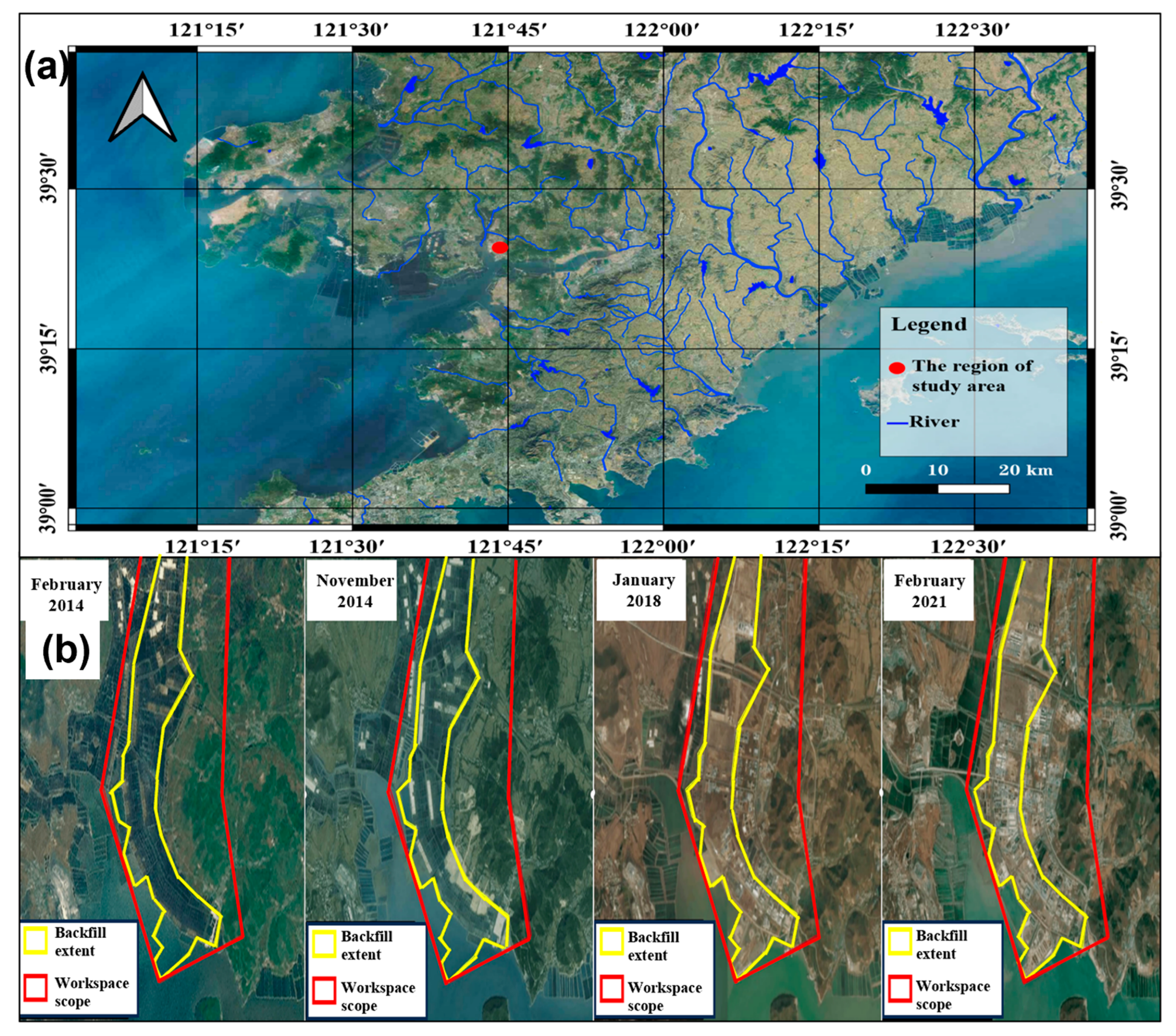
Figure 2.
(a) The distribution of hydrogeological map; (b) comprehensive lithology column chart of backfill area.
Figure 2.
(a) The distribution of hydrogeological map; (b) comprehensive lithology column chart of backfill area.
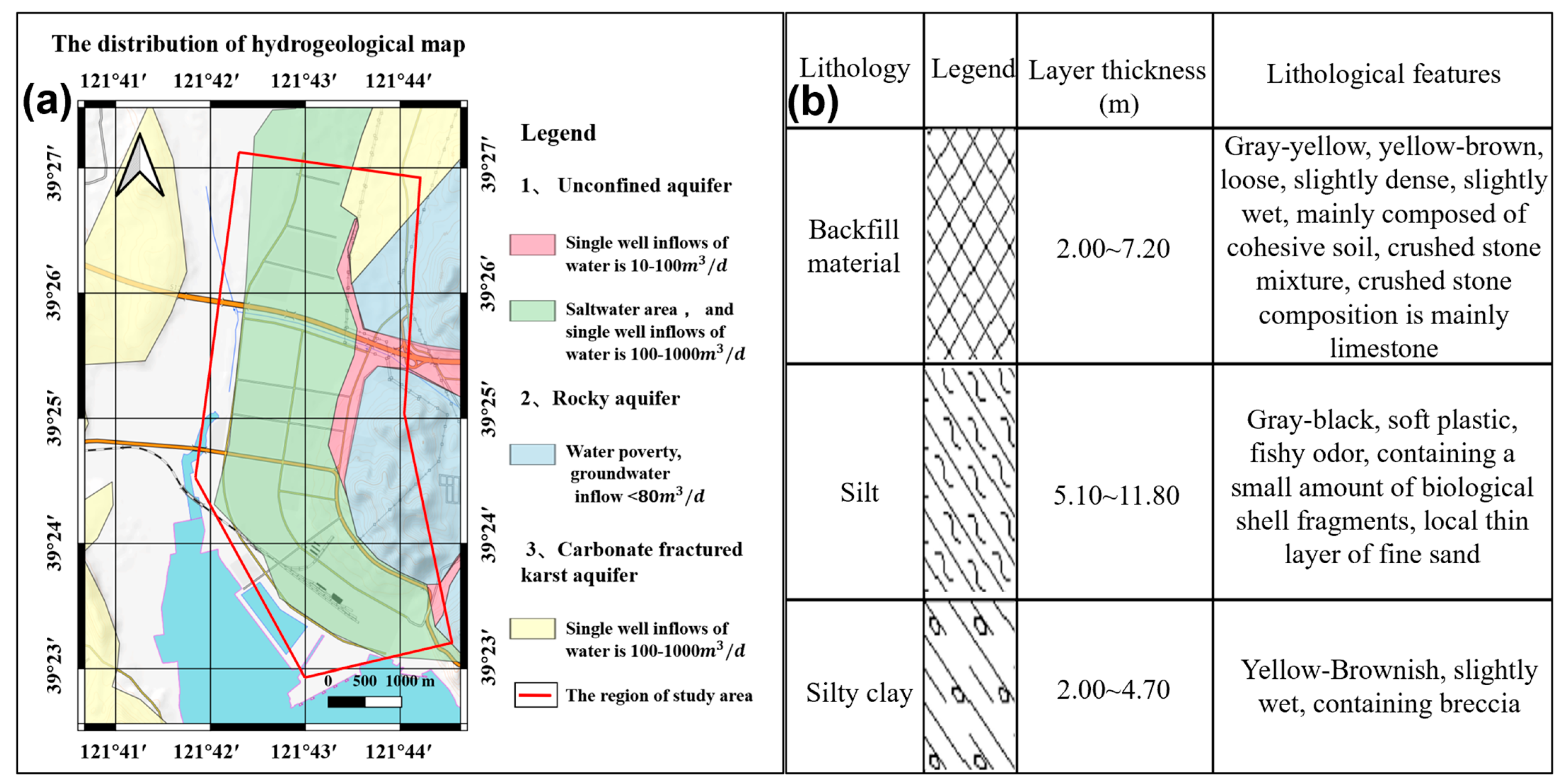
Figure 3.
The distribution of the groundwater monitoring wells.
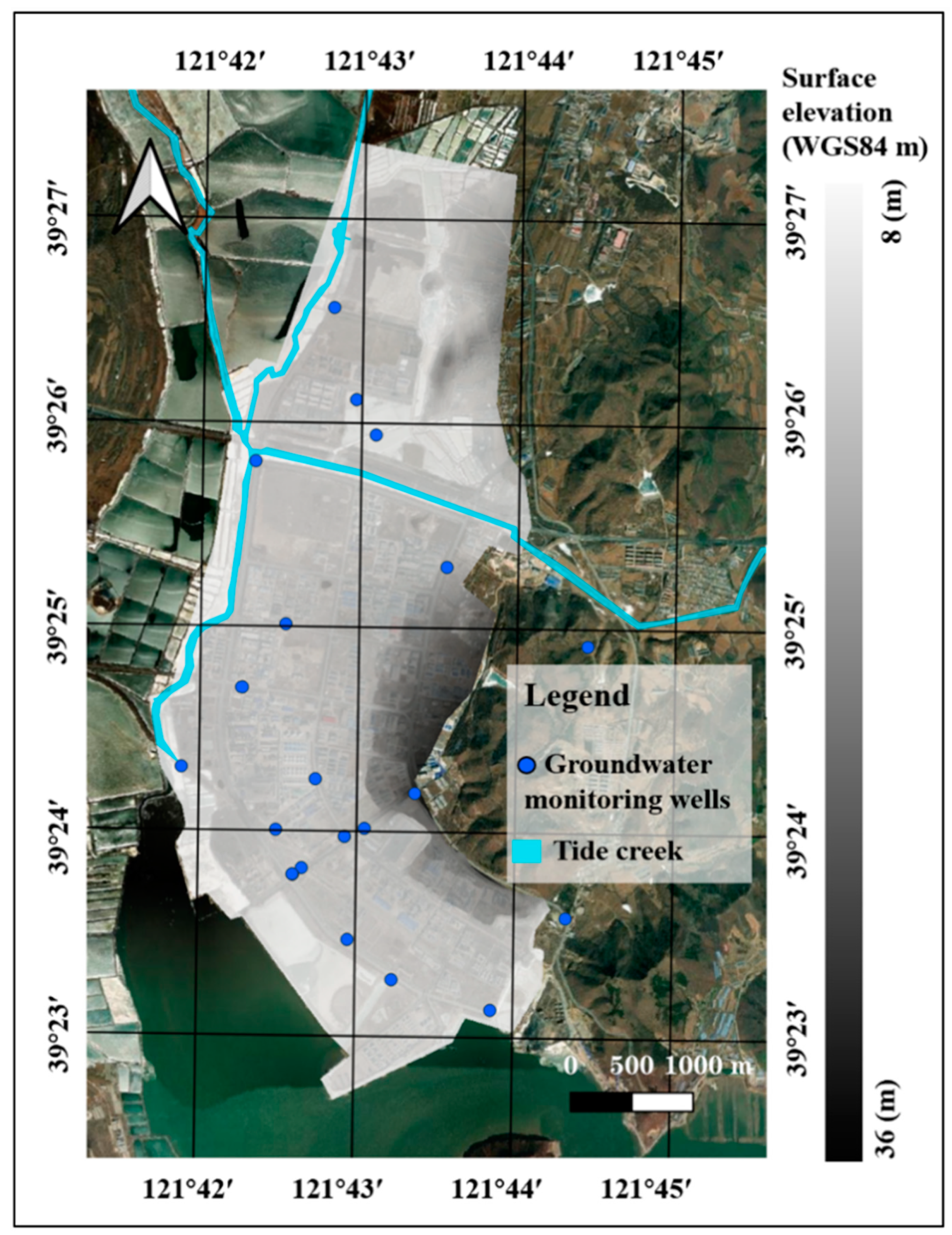
Figure 4.
(a) The configuration of the groundwater monitoring wells; (b) the image showing the drilling cores.
Figure 4.
(a) The configuration of the groundwater monitoring wells; (b) the image showing the drilling cores.

Figure 5.
(a) The data log for the pressure, salinity, and temperature measurement; (b) the YSI@ instrument measures the parameters of groundwater; (c) the image of the slug test; (d) slug test water level change data.
Figure 5.
(a) The data log for the pressure, salinity, and temperature measurement; (b) the YSI@ instrument measures the parameters of groundwater; (c) the image of the slug test; (d) slug test water level change data.

Figure 6.
(a) The distribution of the groundwater table in November 2022; (b) the distribution of the groundwater salinity in November 2022.
Figure 6.
(a) The distribution of the groundwater table in November 2022; (b) the distribution of the groundwater salinity in November 2022.
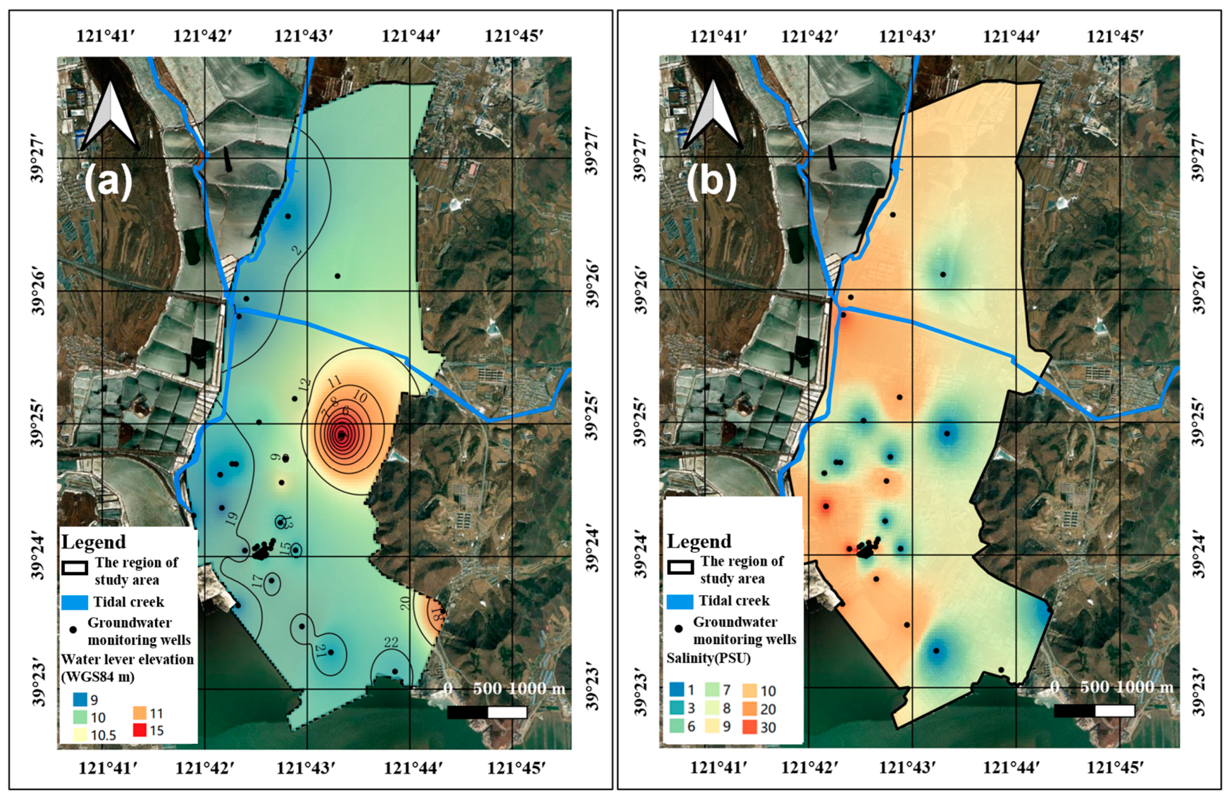
Figure 7.
The distribution of tide and corresponding groundwater oscillation at well with the distance of 100 m to the coastline; the elevation is in WGS84.
Figure 7.
The distribution of tide and corresponding groundwater oscillation at well with the distance of 100 m to the coastline; the elevation is in WGS84.
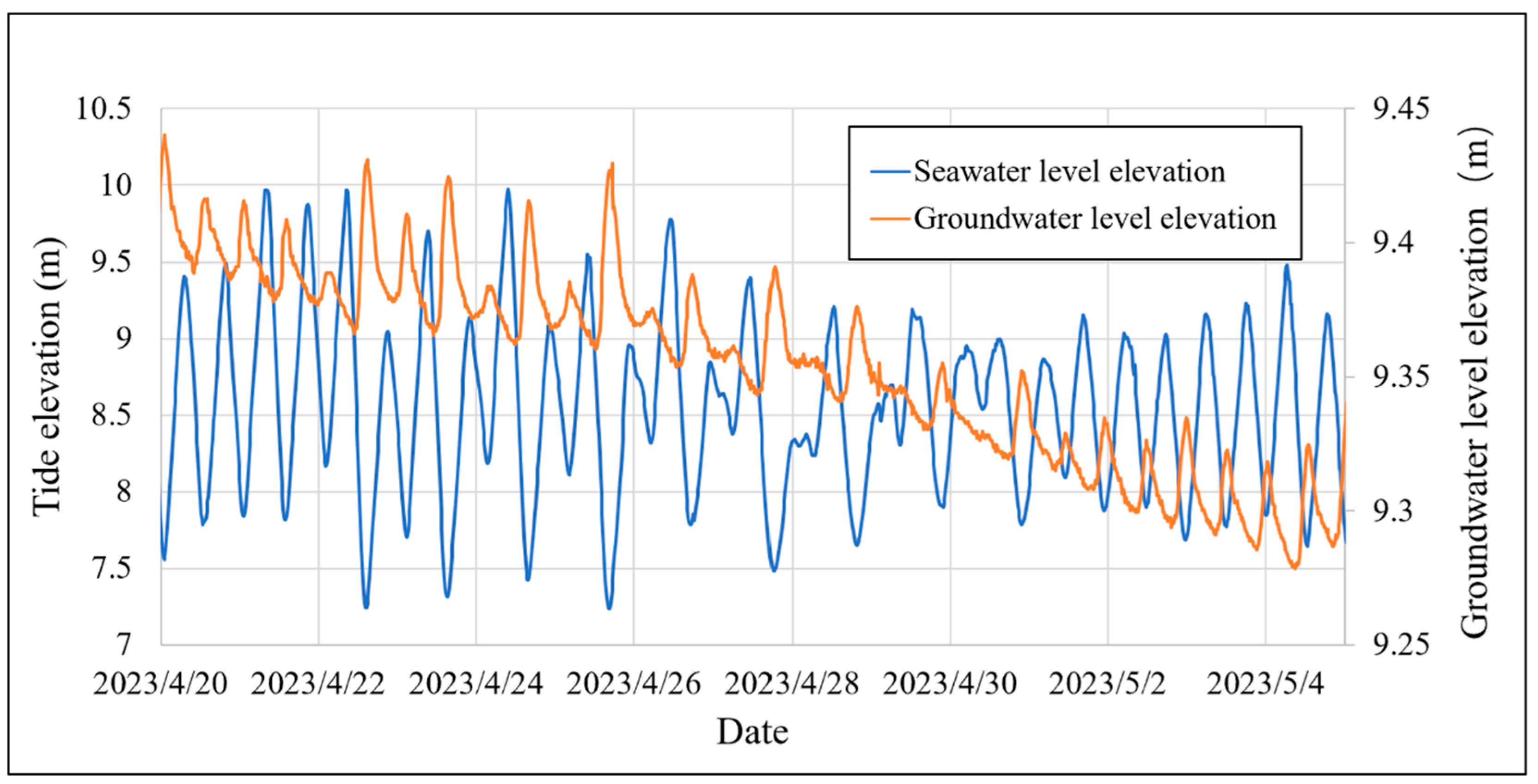
Figure 8.
(a) The distribution of tide and corresponding groundwater salinity at the well with the distance of 100 m to the coast; the elevation is in WGS84, (b) and the oscillation of the seawater salinity and corresponding groundwater salinity at the well with the distance of 100 m to the coast.
Figure 8.
(a) The distribution of tide and corresponding groundwater salinity at the well with the distance of 100 m to the coast; the elevation is in WGS84, (b) and the oscillation of the seawater salinity and corresponding groundwater salinity at the well with the distance of 100 m to the coast.
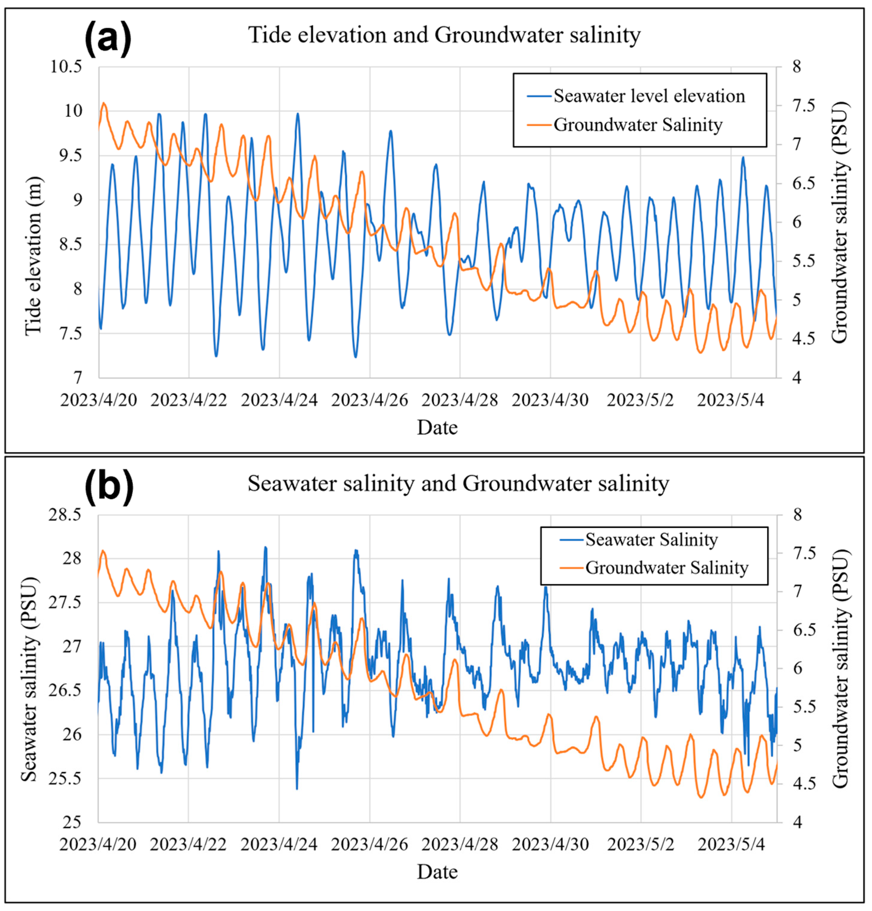
Figure 9.
Measured tide and mainly tides.
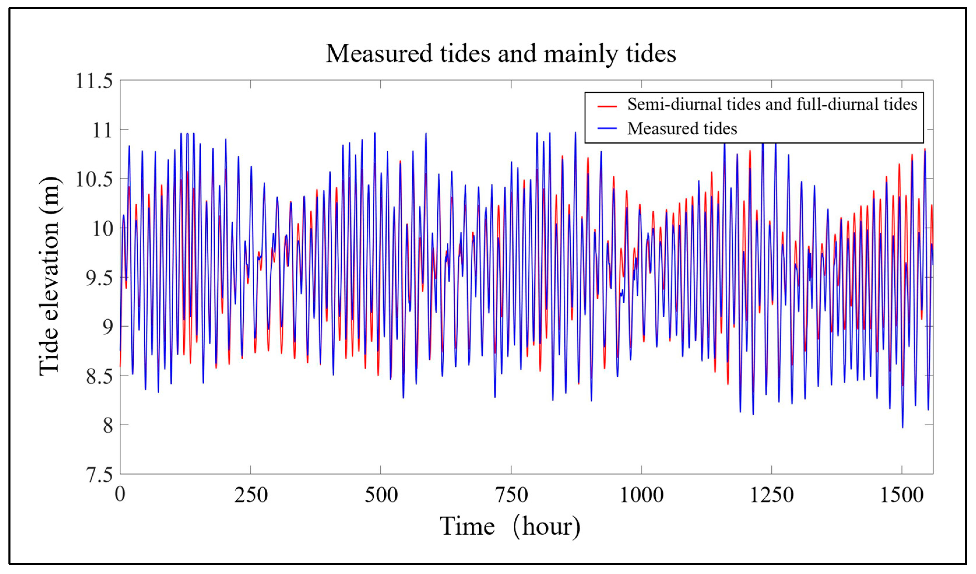
Figure 10.
The harmonic analysis at the well with a distance of 100 m to the coastline; (a) harmonic analysis for the groundwater level; (b) the harmonic analysis for the groundwater salinity.
Figure 10.
The harmonic analysis at the well with a distance of 100 m to the coastline; (a) harmonic analysis for the groundwater level; (b) the harmonic analysis for the groundwater salinity.
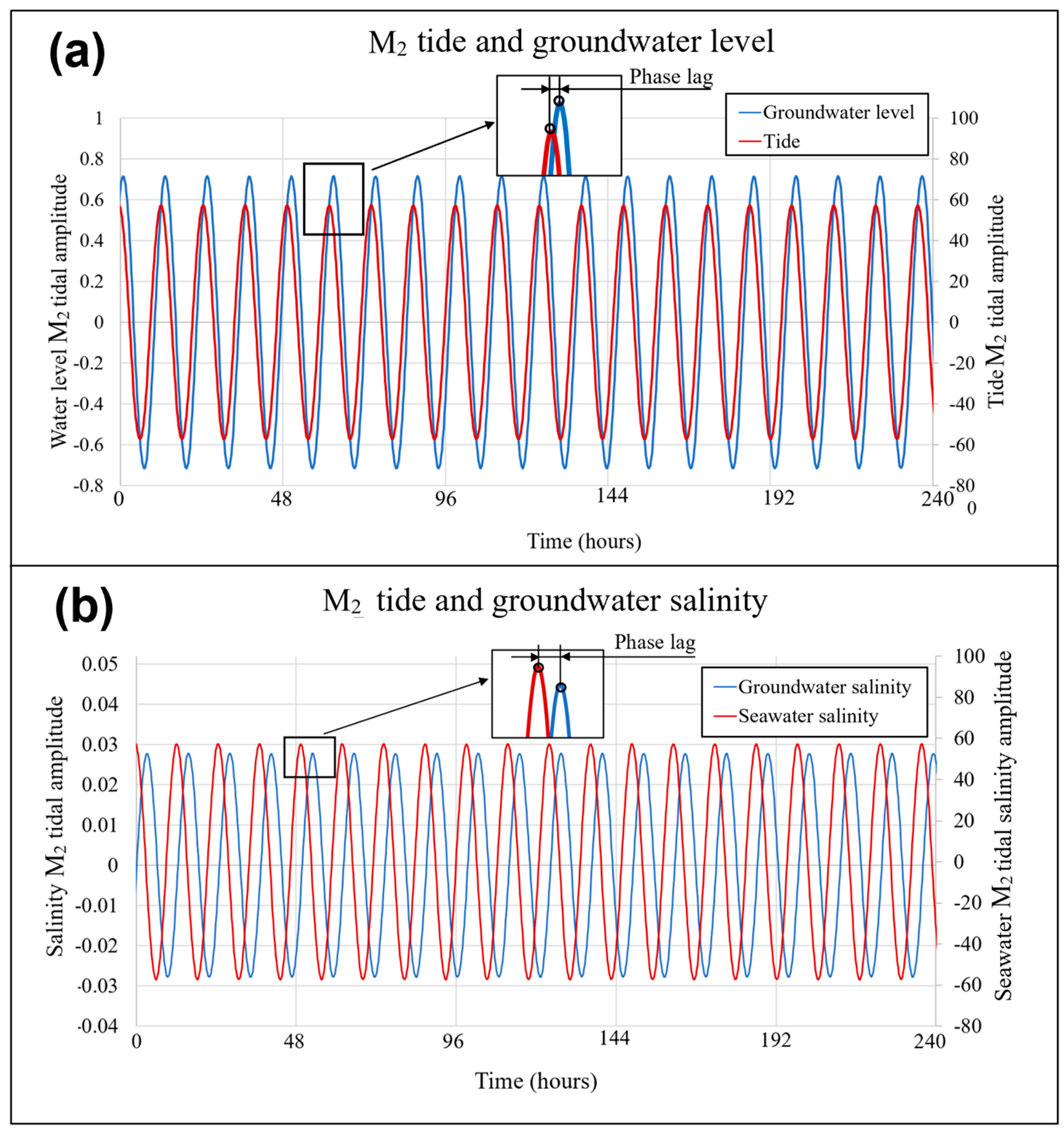
Figure 11.
(a) The harmonic analysis for the groundwater level at three monitoring wells with different distances to the coast; (b) the harmonic analysis for the groundwater salinity at three monitoring wells with different distances to the coast.
Figure 11.
(a) The harmonic analysis for the groundwater level at three monitoring wells with different distances to the coast; (b) the harmonic analysis for the groundwater salinity at three monitoring wells with different distances to the coast.


Table 1.
The result of the harmonic analysis for both groundwater level and salinity at different wells.
Table 1.
The result of the harmonic analysis for both groundwater level and salinity at different wells.
| Phase Lag: (h) | Constituents of Tide | Well (100 m to Coastline) | Well (550 m to Coastline) | Well (1070 m to Coastline) |
|---|---|---|---|---|
| Water level | M2 | 7.2 | 7.4 | 16.4 |
| S2 | 7.1 | 8.7 | 12.2 | |
| K1 | 11.9 | 12.0 | 12.9 | |
| O1 | 12.7 | 13.3 | 26.9 | |
| Salinity | M2 | 14.1 | 13.4 | 15.6 |
| S2 | 13.1 | 16.5 | 12.7 | |
| K1 | 25.2 | 47.7 | 39.1 | |
| O1 | 27.3 | 35.3 | 45.3 |
Disclaimer/Publisher’s Note: The statements, opinions and data contained in all publications are solely those of the individual author(s) and contributor(s) and not of MDPI and/or the editor(s). MDPI and/or the editor(s) disclaim responsibility for any injury to people or property resulting from any ideas, methods, instructions or products referred to in the content. |
© 2023 by the authors. Licensee MDPI, Basel, Switzerland. This article is an open access article distributed under the terms and conditions of the Creative Commons Attribution (CC BY) license (https://creativecommons.org/licenses/by/4.0/).
Share and Cite
MDPI and ACS Style
Guo, J.; Ma, Y.; Ding, C.; Zhao, H.; Cheng, Z.; Yan, G.; You, Z. Impacts of Tidal Oscillations on Coastal Groundwater System in Reclaimed Land. J. Mar. Sci. Eng. 2023, 11, 2019. https://doi.org/10.3390/jmse11102019
AMA Style
Guo J, Ma Y, Ding C, Zhao H, Cheng Z, Yan G, You Z. Impacts of Tidal Oscillations on Coastal Groundwater System in Reclaimed Land. Journal of Marine Science and Engineering. 2023; 11(10):2019. https://doi.org/10.3390/jmse11102019
Chicago/Turabian StyleGuo, Jing, Ye Ma, Chao Ding, Huawen Zhao, Zhixin Cheng, Guanxi Yan, and Zaijin You. 2023. "Impacts of Tidal Oscillations on Coastal Groundwater System in Reclaimed Land" Journal of Marine Science and Engineering 11, no. 10: 2019. https://doi.org/10.3390/jmse11102019
Note that from the first issue of 2016, this journal uses article numbers instead of page numbers. See further details here.