The Black Sea Zooplankton Mortality, Decomposition, and Sedimentation Measurements Using Vital Dye and Short-Term Sediment Traps

Abstract

The principal objectives of this research are to measure the non-consumptive mortality rate of marine copepod zooplankton and the sedimentation rate of copepod carcasses, using short-term sediment traps, and to reveal a correlation between the rates of the two competitive processes—sedimentation and degradation of the carcasses under turbulent mixing conditions. The traps were moored in Sevastopol Bay and adjacent coastal waters (the Black Sea) during summer and autumn seasons. A simulation model was developed to describe a wide range of processes in the trap and the water column above it and to interpret the results obtained with the sediment traps. Significant changes in the abundance of copepod carcasses (from 280 to 12,443 ind. m⁻³) and their fraction in the total zooplankton abundance (53 to 81%) were observed in the waters over short time periods, indicating a high variability of zooplankton mortality, sedimentation, and decomposition rates. Despite the high concentrations of copepod carcasses in the water column, the rates of their accumulation in the traps proved to be extremely low, which could be due to intense turbulent mixing of the waters. The carcass sedimentation rate and the flow of swimmers (motile copepods) into the traps were significantly higher in waters subjected to weaker turbulent mixing. The obtained estimates of the sedimentation rate of copepod carcasses (0.012 to 0.39 d⁻¹) were comparable in value with the rate of their microbial decomposition (0.13 and 0.05 d⁻¹ in the bay and adjacent waters, respectively). This confirmed the hypothesis on microbial decomposition as one of the key controls of the fraction of live zooplankton organisms in zooplankton.

1. Introduction

Zooplankton are essential components of the marine food web, mediating the flow of primary production upwards to higher trophic levels [1], and directly affecting pelagic fish populations and the biological pump of carbon into the deep ocean [2]. Marine ecosystems were shown to be quite sensitive to zooplankton mortality which can modify elemental fluxes into the ocean abyss and alter the balance of pelagic assemblages [2,3]. So, it is crucial to improve zooplankton viability assays, develop the methods for reliable measurement of mortality rate, and have a good understanding of the processes associated with zooplankton mortality and carcass decomposition in the water column.

Dead plankton organisms, including copepod carcasses, have long been the object of hydrobiological research. Various reasons for the plankton mortality, from starvation and disease to algal bloom and environmental pollution, were also of great interest [4,5,6,7,8]. Nevertheless, there are hardly any studies on the linkage of such important phenomenon as non-consumptive (non-predatory) mortality of zooplankton to pollution and trophic status of marine waters. The rate of this process is very difficult to measure in situ due to a number of methodological complications [9]. This is the reason why researchers focus mainly on indirect indicators which include the fraction of live organisms (FLO) in the community. They identify and enumerate dead (or live) organisms, using simple and, to a great extent, subjective methods (light microscopy and visual identification) for calculating the live/dead organisms ratio [6,9,10,11]. The main innovations are aimed at automated methods to study abundance and taxonomic composition of plankton, applying such instruments as Zooscan, ZooCAM, and FlowCAM [12,13]. But the potential of these technologies to assess FLO and study the plankton mortality has not been fulfilled yet. In our research, we used a novel fluorescent marker, diacetate fluorescein (FDA), and an original method of semi-automated (i.e., excepting any subjectivity) sorting of live organisms in zooplankton samples [14,15].

Our previous evaluations of the mortality of dominant crustacean plankton in Sevastopol Bay and adjacent waters [14] have revealed that the mean annual FLO was higher in more polluted waters of the bay corner. On the contrary, in more clean waters outside the bay, FLO was low. In order to explain the contradiction between these results and the already well-established (and seemingly obvious) idea that pollution leads to the death of organisms and, accordingly, to a decrease in FLO [16], we put forward and experimentally confirmed the hypothesis of a more intense bacterial decomposition of dead organisms in the polluted and eutrophicated waters of the bay and, as a possible consequence, an increase in FLO [15]. Indeed, a pool of dead organisms is formed as a result of natural (non-consumptive) mortality of zooplankton, while carcasses are removed from the water column due to the two main processes: bacterial degradation [6] and sedimentation [4,17].

The sedimentation rate of dead organisms is measured in situ based the rate of their accumulation in sediment traps installed near the bottom in different water areas [5,9,18,19]. However, the majority of such investigations were carried out in calm fresh waters where sedimentation is the main way of removal of the carcasses from the water column. Consequently, other contributing factors, such as carcass degradation, were neglected, supposing that their sedimentation occurs faster than their degradation [8,18,19]. But a series of other studies demonstrated that under turbulence and stratification, dead zooplankton may get suspended in the water column and act as an additional source of matter and energy for bacteria [20,21].

Turbulent mixing of water, utilization of carcasses by detritophages, and their decomposition by bacteria are among the processes which are commonly ignored by the researchers of zooplankton mortality making the methods they use unreliable. In this study, we just tried to overcome some of these difficulties by developing an appropriate simulation model describing the processes in the sediment trap more precise. The principal objectives of our research are to measure the non-consumptive mortality rate of the copepod zooplankton and the sedimentation rate of copepod carcasses, and to reveal a correlation between the rates of the two competitive processes—sedimentation and degradation of the carcasses, which determine the FLO dynamics under turbulent mixing conditions.

2. Materials and Methods

2.1. Study Sites and Experimental Design

A total of three series of experiments were carried out in the coastal waters of the SW Crimea (the Black Sea). The experiment BAY11 was run at Station B in Sevastopol Bay on 28–30 November 2017. The experiments SEA05 and SEA11 were conducted at Station S in the adjacent waters (a mile off the entrance to the bay, with the depth down to 40 m) on 30–31 May 2017 and 16–23 November 2017, respectively (Figure 1).

The areas chosen for the research differ considerably in pollution level and trophic status. Sevastopol Bay is located at the south-western part of the Crimean Peninsula (the Black Sea). It is a semi-enclosed estuary-type body of water with a reduced water renewal rate (because of a mole at the entrance) and exposure to chronic industrial and anthropogenic stress. From the mouth of the Chernaya river in the corner of the bay (St. B) to the open water outside the bay (St. S) there were observed a gradual increase in water salinity, and a decrease in the levels of pollution and trophicity. Waters of the bay are characterized by high concentrations of nutrients, several times exceeding their background readings in the open sea: up to 290 µmol L⁻¹ of nitrite nitrogen, up to 6.4 µmol L⁻¹ of nitrate nitrogen, up to 41 µmol L⁻¹ of ammonium nitrogen, up to 5.2 µmol L⁻¹ of phosphates, up to 98 µmol L⁻¹ of silicates [23]. The eutrophication E-TRIX index was shown to change on average from 5.05 in the bay at St. B to 4.70 in the open sea at St. S, characterizing the level of trophicity of Sevastopol Bay as a transition from medium to high [24]. Chronic oil pollution level increases from the open waters outside the bay to its central part. In particular, the total amount of chloroform extractable organic compounds ranges from 0.9 to 26.8 mg g⁻¹ of air-dried bottom sediments. The highest oil pollution levels are revealed in the central part of the bay, with a maximum concentration of 13.4 mg g⁻¹ [25].

Temperature and wind condition at the stations were also different during the trap deployment. At St.S, water surface temperature was 19.1 °C and remained unchanged through the exposition time of the trap during the experiment SEA05. Wind speed did not exceed 2.3 m s⁻¹, its direction changed from eastern to north-western. In November (SEA11 experiment), north-eastern winds prevailed with gusts up to 5–7 m s⁻¹, water surface temperature decreased from 13.4 °C to 11.9 °C during the 7-day trap exposition. At St. B in the bay (BAY11 experiment), average wind speed was 3 m s⁻¹, and temperature increased from 11.0 °C to 12.4 °C.

2.2. Design and Exposure Conditions of Sediment Traps

According to [22], the trap tube unit was custom-made of a 120-cm long plastic tube with entry-hole diameter of 110 mm (Figure 1A). The funnel was a 2-L plastic bottle, mounted on a pipe and by means of a screwed joint connector attached to a collection cup (0.5-L plastic bottle). The sediment trap in full assembly included four fastened tube units.

The traps were moored as close to the bottom as possible, anchoring the device with a 30-kg load at the depth of 8 m at St. B in the bay (BAY11 experiment) and 16–36 m at St. S in the open sea (SEA05 and SEA11 experiments). In order to keep the trap vertical, a submerged buoy was used. The trap location was marked with a signal buoy on the water surface.

Since few zooplankton carcasses were found in the traps after the 24-h experiment (SEA05), the trap exposition had to be prolonged from 2 (BAY11) to 7 (SEA11) days. Thus, the sediment traps were deployed for 1, 2, and 7 days during the experiments SEA05, BAY11, and SEA11, respectively.

In the experiments SEA11 and BAY11, the collection cups of two units (poisoned units) were filled with 40% formaldehyde (fin. conc. 2%). The other two units of the trap had no preservatives (non-poisoned units). First, the preservative prevented microbial decomposition of copepods in the trap and, second, it killed accidental “swimmers” getting in the trap, thus providing their accumulation in the collection cup. Consequently, a comparison of the data from the poisoned and non-poisoned units allowed us to estimate the two processes, the carcass decomposition rate and the swimming rate of alive copepods into the traps.

The contents of the sediment cups and the trap tubes in the poisoned and non-poisoned units were analyzed independently. Live organisms were identified in the non-poisoned units, using a vital stain (see below). The zooplankton found in the sediment cup of the poisoned unit were considered dead and, hence, were not stained for further viability assay. The contribution of the swimmers to the total abundance of copepods in the poisoned unit was estimated, using a simulation model.

2.3. Evaluation of Total Abundance of Zooplankton and Fraction of Live Organisms (FLO)

To study zooplankton species composition, abundance, and FLO, samples of zooplankton were taken at the trap location with a Juday net (entry-hole diameter 37 cm, 150-μm mesh, filtering cod end) at the beginning of the experiment, immediately after the trap deployment, and after its exposition.

Zooplankton samples from the water column above the trap and all the trap units were studied under a light microscope according to [26,27]. The abundance of live and dead organisms was evaluated after staining the samples with fluorescein diacetate (FDA), following the original protocol [14,28]. The FDA solution was prepared in dimethyl sulfoxide (DMSO) (5 mg mL⁻¹) and stored at +4 °C. For FDA staining, 1 μL of FDA solution was added to 1 mL of sample material according to the method widely used in marine phytoplankton research [29]. The sample was stained for 40 min in the dark. Earlier, this fluorescent stain was first used in field studies of marine zooplankton as viability marker in a series of our studies [14,28,30].

Organisms were microphotographed in a Bogorov’s glass chamber under an inverted microscope (Nikon Eclipse TS100-F) (×4, ×10) equipped with a photo- and video camera (Ikegami ICD-848P) in the fluorescent mode (blue excitation filter set). The obtained images were processed with ImageRegionColor (IRC) software for semi-automated estimation of the proportions of the live and dead zooplankton. The updated version IRC 2.0.2. developed specifically for our tasks includes discriminant analysis, and allows statistically significant differentiation between dead and live organisms, depending on intensity of their staining.

2.4. Estimation of Abundance and Physiological Activity of Bacteria

Flow cytometry was used for measuring the total abundance of bacteria in the water column and collection cups of the trap at the beginning and after the trap exposition. Bacterial cells were counted with a Beckman Coulter flow cytometer (Cytomics FC 500) equipped with blue laser (15 mW, 488 nm). Aliquots (1 mL) of water samples previously preserved in formaldehyde (fin. conc. 2%) were stained with SYBR Green I (Molecular Probes Inc.) following the procedures described in [31,32]. Fluorescence of SYBR-Green I in the FL1 green light (525 nm) was assumed to be proportional to the content of intracellular nucleic acids and was interpreted as a measure of specific metabolic activity of bacterial cells, according to [33]. The nonparametric Mann–Whitney test was used to compare seasons and locations in terms of zoo- and bacterioplankton abundances. The significance level for all tests was set at <0.05.

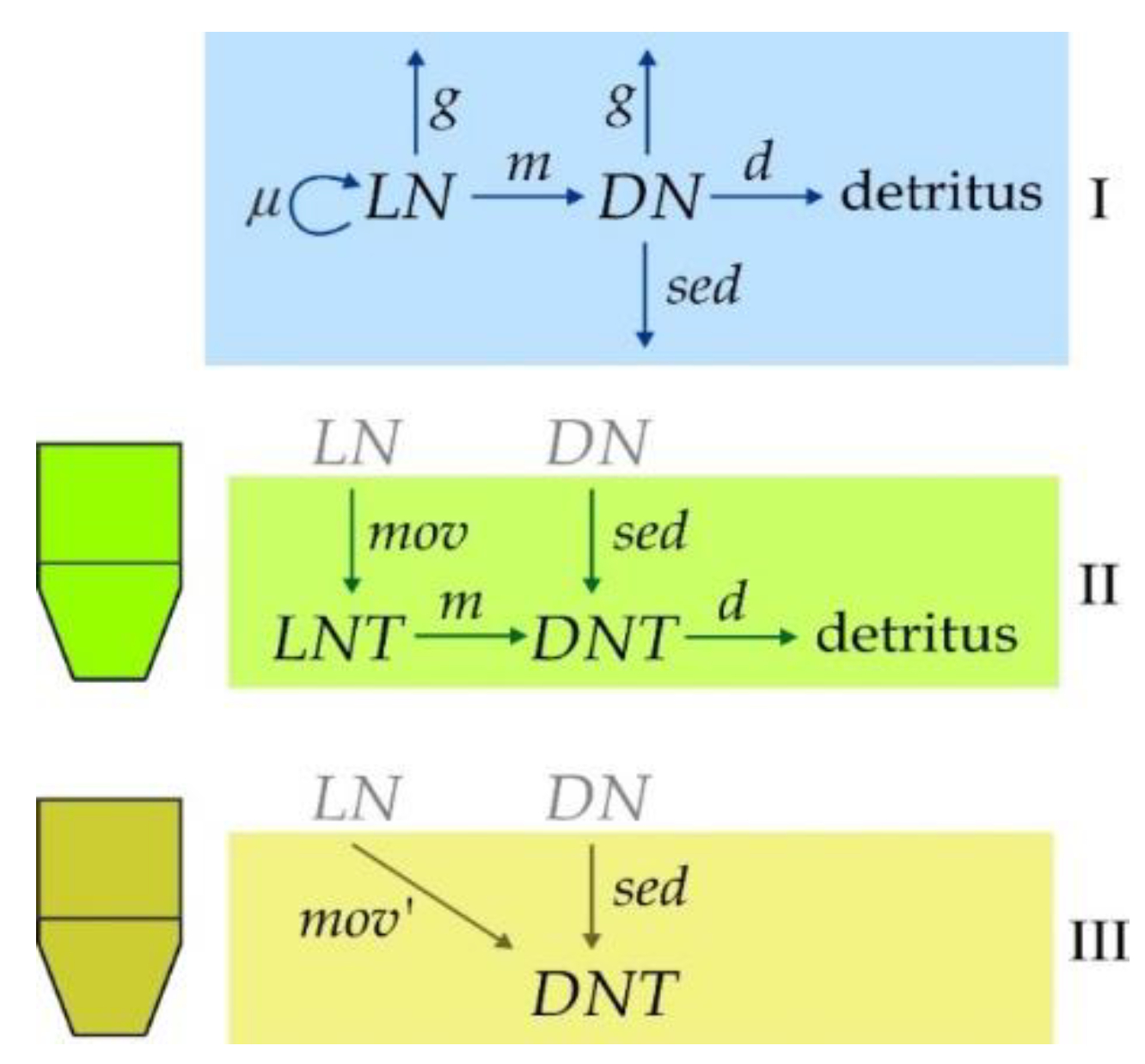
2.5. Simulation Model of Live and Dead Zooplankton Dynamics in Sediment Traps and Water Column above Them

A simulation model was developed to comprehend and interpret the results of the field experiments, and estimate the matter flows through the community, including consumptive and non-consumptive mortalities, sedimentation, and decomposition. The model included three spatially homogeneous sub-models for describing live and dead copepod zooplankton dynamics (i) in the water column above the trap (Figure 2, I), (ii) in the non-poisoned units (Figure 2, II), and (iii) in the poisoned units (Figure 2, III).

Table 1. List of the measurable variables (*) and the model parameters.

Symbol	Description	Units
N0	Initial zooplankton abundance in the water column *	ind. M−3
Nt	Final zooplankton abundance in the water column *	ind. M−3
FLO	Fraction of live organisms *	%
LN	Abundance of live organisms in the water column above the trap	ind. M−3
LN0	Initial abundance of live copepods in the water column above the trap *	ind. M−3
LNt	Final abundance oflivecopepodsin the watercolumnabovethetrap *	ind. M−3
rlive	Apparent specific rate of growth/loss of live copepods *	d−1
rdead	Apparent specific rate of production/loss of dead copepods *	d−1
DN	Abundance of dead copepods in the water column above the trap	ind. M−3
DN0	Initial abundance of dead copepods in the water column above the trap *	ind. M−3
DNt	Final abundance of dead copepods in the water column above the trap *	ind. M−3
LNT	Abundance of live organisms (swimmers) in the trap *	ind.
DNT	Abundance of carcasses in the trap *	ind.
M	Non–consumptive mortality rate	d−1
g	Consumptive mortality rate	d−1
d	Carcass decomposition rate	d−1
µ	Specific growth rate	d−1
sed	Sedimentation rate	d−1
mov	Net flow of swimmers into the non–poisoned trap unit	d−1
mov’	Net flow of swimmers into the poisoned trap unit	d−1
T	Duration of the experiment	d

provides description and units for all the variables measured in the field experiments, as well as the model parameters.

The first sub-model (Figure 2, I) described dynamics of live (LN) and dead (DN) copepods in the water column above the trap and included specific growth rate of their populations (µ), non-consumptive (m), and consumptive mortality (g), as well as sedimentation (sed) and decomposition (d) of dead organisms:

$$\frac{dLN}{dt}=\left(\mu -g-m\right) LN$$

(1)

$$\frac{dDN}{dt}=m LN-\left(d+g+sed\right) DN$$

(2)

To simplify the model, a few assumptions were made, including: non-selective consumption of dead and live organisms by predators; equality of the non-consumptive mortality rate (m) in the non-poisoned unit and the above water column; equality of the decomposition rate (d) in the non-poisoned unit and the above water column. The value of d was calculated from previously obtained data (0.13 and 0.05 d⁻¹ at the St. B and St. S, respectively, at 22.0 °C [15]), and the temperature coefficient Q₁₀ = 2.4 [34].

The in situ sedimentation experiments allowed measuring the initial and final abundances of live and dead copepods in the water column above the trap (LN₀, DN₀, LN_t, and DN_t), and consequently, calculating the apparent growth rate of live (r_live) and dead (r_dead) copepods over the duration of the experiment (T):

$$r_{live}=\frac{(ln\left(L{N}_t\right)-\mathit{ln}\left(L{N}_0\right))}{T}$$

(3)

$$r_{dead}=\frac{(ln\left(D{N}_t\right)-\mathit{ln}\left(D{N}_0\right))}{T}$$

(4)

The empirical coefficients r_live and r_dead reflected the entire set of processes occurring in the water column and controlling the population of zooplankton: growth, mortality, sedimentation, and decomposition of organisms. The abundance of dead and live copepods in the water column (LN and DN, respectively) were external parameters for the sub-models II and III, describing processes in the traps. So, it was convenient to describe their dynamics with the equations:

$$\frac{dLN}{dt}=r_{live }LN$$

(5)

$$\frac{dDN}{dt}=r_{dead }DN$$

(6)

The sub-model II simulated the processes in the non-poisoned units of the trap (Figure 2, II). Apart from the copepod carcasses (DNT) sinking into the trap from the water column (sed) and suffering from bacterial decomposition there (d), the model took into account the accumulation of the live swimmers in the trap (LNT), their non-consumptive mortality (m), and decomposition of the carcasses (d) in the trap:

$$\frac{dDN}{dt}=m LNT+sed DN-d DNT$$

(7)

$$\frac{dLNT}{dt}=mov LN-m LNT$$

(8)

As it was stated above, the “external” variables LN and DN were defined from the Equations (5) and (6), using the empirical coefficients r_live and r_dead (the Equations (3) and (4)). Since the model did not account for the swimmers getting from the trap back to the water column, the coefficient mov presented the balance between inflow and outflow of the swimmers in/out the trap. Consequently, it appeared to differ significantly in the poisoned and non-poisoned units, and depend on behavior of the zooplankton. For example, organisms might have been attracted into the trap by excess of food or avoided the toxic content of the trap. On the contrary, the rates of sedimentation and accumulation of carcasses in both the units were supposedly the same.

The third sub-model (Figure 2, III) described dynamics of dead organisms (DNT) in the poisoned unit as a function of live (LN) and dead (DN) copepods abundance in the water column above the trap, net flow of the swimmers in/out the trap (mov’) and sedimentation of copepod carcasses from the water column (sed):

$$\frac{dDNT}{dt}={mov}^{\prime }LN+sed DN$$

(9)

Live organisms were absent in the poisoned unit according to the assumption that all the swimmers were immediately killed by formaldehyde (mov’ × LN in the Equation (9)). For the same reason, copepod carcasses were not decomposed by bacteria whose activity was depressed by the fixator (d × DNT is absent in the Equation (9)). Same as in the sub-model II, the “external” variables LN and DN were defined from Equations (5) and (6).

Numerical experiments were carried out sequentially with each of the sub-model from III to I in such a way as to determine the ranges of the coefficients at which the dynamics of zooplankton in the water column and the traps would correspond well to the empirical data obtained during the experiments. For the same estimates of sed obtained in the sub-models II and III, the flow of the swimmers into the poisoned (mov’) and non-poisoned (mov) trap units were calculated and compared. Next, mortality (m) and sedimentation (sed) variability and interrelations were studied in the sub-model II. The values and nature of the relationship between these coefficients were used later in the sub-model I in order to calculate the specific growth rate (µ) and consumptive mortality (g) of zooplankton.

3. Results

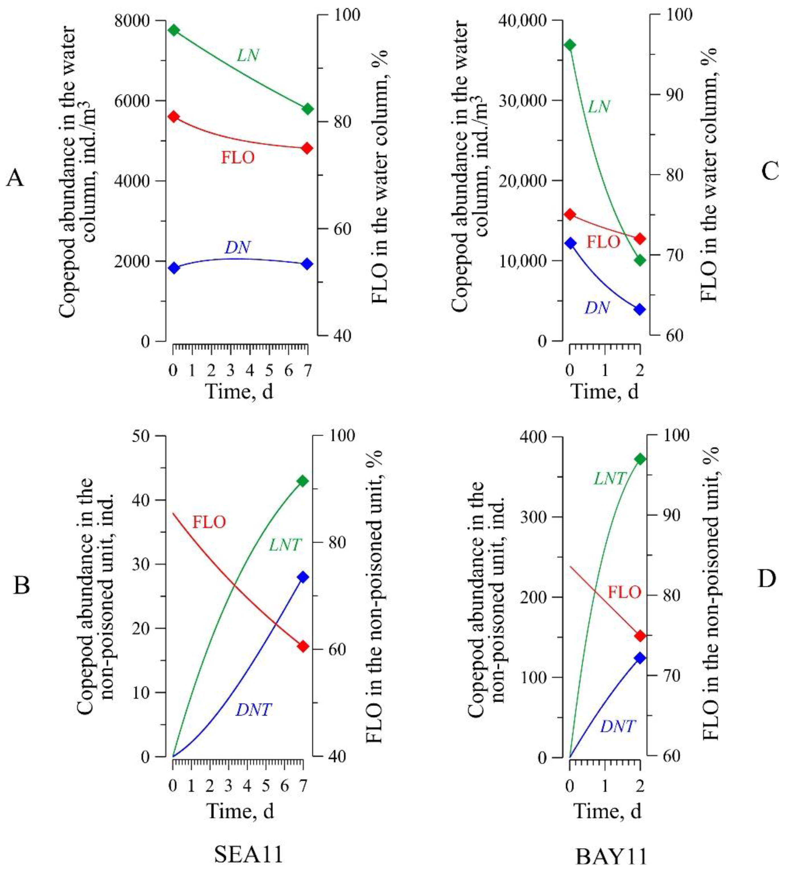
3.1. Species Composition and Dynamics of Zooplankton in the Water Column above the Sediment Trap

In the samples taken in May in the open sea (the experiment SEA05), the heterotrophic dinoflagellate Noctiluca scintillans dominated the community (

Table 2. Initial (N₀) and final (N_t) total abundances of zooplankton and the fraction of live organisms (FLO₀ and FLO_t, resapectively) in the water column, and the numbers of live (LNT) and dead (DNT) organisms found in the poisoned and non-poisoned trap units after their exposition.

Taxon	Water Column		Water Column		Non-Poisoned Unit		Poisoned Unit
	N0, ind. m−3	FLO0, %	Nt, ind. m−3	FLOt, %	LNT, ind.	DNT, ind.	LNT, ind.	DNT, ind.
Experiment SEA05 (St. S; depth: 36 m; time of exposition: 1 day)
Total Copepoda	Nd *	53	849	67	12	0	–	–
Acartia clausi	nd	58	554	65	2	0	–	–
Pseudocalanus elongatus	nd	52	36	71	4	0	–	–
Oithona similis	nd	49	177	60	5	0	–	–
Copepoda nauplii	nd	88	144	94	10	1	–	–
Pleopis polyphemoides	nd	nd	29	nd	1	0	–	–
Noctiluca scintillans	nd	nd	7806	nd	5	0	–	–
Cirripedia nauplii	nd	nd	188	nd	3	1	–	–
Bivalvia larvae	nd	nd	87	nd	2	0	–	–
Experiment SEA11 (St. S; depth: 16 m; time of exposition: 7 d)
Total Copepoda	9597	81	6181	75	43	28	0	178
Acartia clausi	801	87	1527	94	1	0	0	3
Paracalanus parvus	1858	67	1433	43	5	1	0	91
Oithona similis	445	88	203	47	0	0	0	7
Oithona davisae	2435	86	2859	86	10	11	0	32
Harpacticoida	0	nd	2	nd	27	4	0	19
Copepoda nauplii	861	100	797	95	10	7	0	21
Oikopleura dioica	0	85	0	nd	0	0	0	6
Bivalvia larvae	56	nd	135	nd	0	0	0	15
Experiment BAY11 (St. B; depth: 8 m; time of exposition: 11 d)
Total Copepoda	49,691	75	13,981	72	372	125	0	1054
Acartia clausi	237	87	309	64	2	1	0	3
Paracalanus parvus	1707	32	459	4	0	1	0	11
Pseudocalanus elongatus	926	71	60	0	0	3	0	54
Pseudodiaptomus marinus	0	0	0	0	64	2	0	30
Oithona similis	250	89	75	nd	0	0	0	3
Oithona davisae	46,312	84	13,012	91	285	93	0	854
Harpacticoida	1,25	nd	0	nd	21	3	0	25
Copepoda nauplii	40	nd	89	nd	13	0	0	43
Cirripedia nauplii	584	nd	350	nd	8	2	0	12
Oikopleura dioica	0	nd	112	nd	0	0	0	19
Bivalvia larvae	1229	nd	131	nd	0	0	0	22
Polychaeta larvae	40	nd	62	nd	1	0	0	39
Gastropoda larvae	90	nd	44	nd	0	0	0	5

* nd—no data.

). Copepods were rare and presented by the eurythermal species Acartia clausi, the cold-water Oithona similis, and Pseudocalanus elongatus. In November, all the water samples collected during both the experiments (BAY11 and SEA11) were dominated by copepods. In particular, the invasive cyclopoid copepod Oithona davisae was highly abundant, that is a common species in coastal waters of the Black Sea in autumn [35]. Additionally, Paracalanus parvus, P. elongatus, A. clausi, and nauplii were found at both the stations. Meroplankton were represented by Bivalvia, Polychaeta, Cirripedia, Gastropoda, and Decapoda. These taxa were more abundant in the bay samples (Table 2).

In November, the total abundance of copepods in the water column above the trap was significantly lower at St. S (below 10⁴ ind. m⁻³) than at St. B (about 5 × 10⁴ ind. m⁻³) (Table 2). Over the two-day experiment BAY11 at St. B, the total abundance of copepods (and some other zooplankton groups) was decreasing more than three-fold, from 5.0 to 1.4 × 10⁴ ind. m⁻³, mostly due to the dominant species O. davisae. Such great changes in the zooplankton numbers could have been related to their abnormally high mortality rates, which was supposed to be verified using the model. But a transfer of the plankton with water masses also could not be excluded as a reason for this phenomenon.

The FLO values obtained for particular groups of zooplankton varied within a wide range from 4 to 100%, and the minima being registered in a few species of copepods, including the abundant P. parvus (Table 2). This species was found in November at both the stations, while its live individuals made up only 4% in the samples from the bay. On the contrary, FLO reached as high as 84 to 91% in O. davisae predominant in autumn samples. No carcasses were found among Cirripedia and copepod nauplii.

3.2. Accumulation of Zooplankton in the Sediment Trap

Results from the May pilot project (SEA05) showed that very few zooplankton (including 12 copepods and 10 copepod nauplii) were in the sediment trap after a 24-h exposure. The majority of the organisms in the trap were live (excepting 1 Copepoda nauplius and 1 Cirripedia nauplius) (Table 2). Despite the presence of a significant number of dead copepods in the water column (about 400 ind. m⁻³ of copepods), their absence in the traps indicated an important role of the processes hindering sedimentation of dead zooplankton, such as water mass movement and turbulent mixing. The latter seemed to not affect the ability of actively moving zooplankton to swim in and out of the trap.

When the experiments were extended to 2–7 days in November, it permitted to increase considerably the abundance of carcasses in the traps, especially during mass development of O. davisae (experiment BAY11), up to tens of individuals in the non-poisoned units (Table 2). However, the prolonged time of the trap exposition complicated the processes going on inside it. In particular, the abundance of live swimmers getting in the traps by accident grew considerably. At the same time, the chances of their death inside the trap also increased, which, in its turn, could lead to false mortality and sinking estimates. Thus, both the factors—turbulence and active swimmers—could be the source of miscalculations.

In the November experiments, the abundance of dead copepods in the non-poisoned trap units increased significantly (28 ind. in SEA11, and 125 ind. in BAY11). However, the number of the swimmers remained two to three times higher (43 and 372 ind., respectively). In the poisoned traps, the number of copepods more than doubled (178 ind. in SEA11, and 1054 ind. in BAY11), indicating a considerable proportion of the swimmers and their ability not only to swim into the trap, but also to leave it easily.

Apart from numerous copepods, the non-poisoned units contained live copepod nauplii, as well as single individuals of Cirripedia, larvae of Bivalvia and Polychaeta, while their carcasses were hardly present. The abundance of these organisms (and other taxons like Gastropoda larvae, Decapoda larvae, Oikopleura dioica) in the poisoned units was significantly higher, which was associated with their ability to swim in the trap, same as copepods (Table 2).

An interesting finding was a new and still rare in the Black Sea invasive copepod Pseudodiaptomus marinus [36], a few individuals of which were found in the near-bottom traps in Sevastopol Bay (experiment BAY11). This species is capable of active vertical migrations, while staying in the near-bottom layer during the day, that might explain its occurrence in the traps. Moreover, dozens of harpacticoid copepods were found in the traps exposed close to the bottom as they prefer to live in the near-bottom layer and are associated with seaweeds.

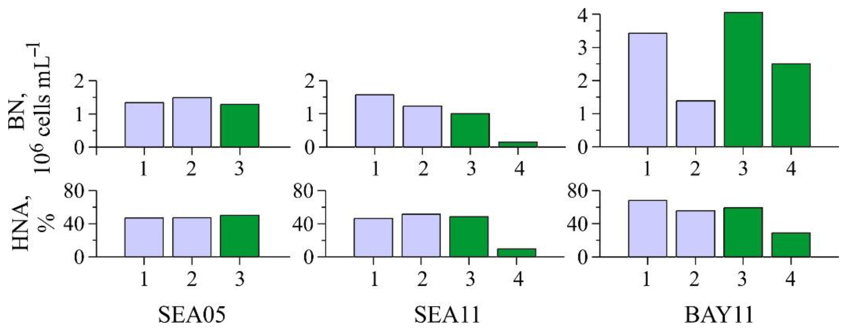
3.3. Dynamics of Bacterioplankton in the Water Column and the Traps

At St. S, bacterioplankton abundances differed insignificantly in May (1.34 × 10⁶ cells mL⁻¹) and November (1.57 × 10⁶ cells mL⁻¹). In the bay, bacteria were more abundant, up to 3.42 × 10⁶ cells mL⁻¹. During the two-day experiment BAY11, the abundance of bacterioplankton decreased down to 1.38 × 10⁶ cells mL⁻¹, thus, changing as considerably as the abundance of the copepod zooplankton (Table 2). This also indicated a complete change in plankton structure as a result of water mass movement over the experiment (Figure 3).

During the experiments SEA05 and SEA11, there was no significant bacterial growth in the non-poisoned units. On the contrary, in the bay (BAY11), where the abundances of bacteria and zooplankton were high, the bacterial numbers in the trap increased up to 4 × 10⁶ cells mL⁻¹. In the presence of the fixative, the total number of bacteria and the proportion of physiologically active bacteria dropped significantly, but the complete death of microorganisms did not occur, probably due to the constant dilution of the fixative during the exposure (Figure 3).

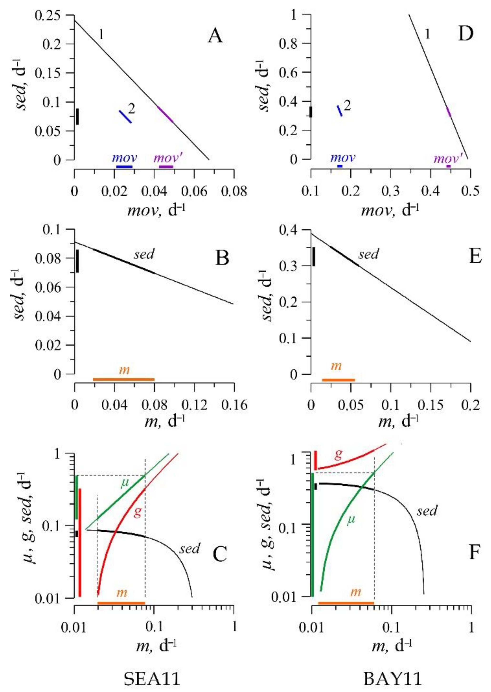
3.4. Results of Numerical Experiments

Application of the simulation model has allowed us to study dynamics and major functional characteristics of zooplankton community, including the predominant species—invasive copepod O. davisae. The results of simulation of the copepod dynamics in the traps and in the water column above them at stations in the bay (BAY11) and in the open sea (SEA11) are presented in Figure 4. In both the numerical experiments, the abundance of live copepods dropped significantly, especially in the bay, while FLO did not decrease much, in the range between 80% and 70% (Figure 4A,C). Inside the non-poisoned trap units, the decrease in FLO was more pronounced due to the high rate of accumulation of carcasses (Figure 4B,D).

Figure 5 represents the ranges of values of the model parameters at which the simulated dynamics of copepods in the water column and traps corresponded well to the empirical data obtained in the experiments SEA11 (Figure 5A–C) and BAY11 (Figure 5D–F). In the sub-model III, dependences were obtained (straight line 1 in Figure 5A,D) between the rates of sedimentation of carcasses (sed) and flow of swimmers (mov’), which determined the accumulation of dead copepods in the poisoned trap unit by the end of the experiments SEA11 (DNT_t = 178 ind.) and BAY11 (DNT_t = 1054 ind.) (Table 2).

The sub-model II (non-poisoned unit) included two additional coefficients—decomposition of carcasses (d) and non-consumptive mortality of the swimmers (m). The values of d were set taking into account the water temperature and the coefficient Q₁₀ and kept unchanged in each of the numerical experiments. For a wide range of values of non-consumptive mortality (m), we studied the dependences (straight line 2 in Figure 5A,D) between the rates of sedimentation of carcasses (sed) and swimming (mov), which determined the accumulation of carcasses and live copepods in the non-poisoned trap unit and ensured compliance model to the empirical data obtained by the end of the experiments SEA11 (LNT_t = 43 ind., DNT_t = 28 ind.) and BAY11 (LNT_t = 372 ind., DNT_t = 125 ind.). Such a correspondence was achievable at much lower values of the swimming rate (mov < mov’), because in the absence of the fixative, mov was the result of two opposite processes—the swimming of organisms into the trap and their swimming out of it. In addition, a relationship between sed and m was obtained in the sub-model II (Figure 5B,E), which was later used in the sub-model III, based on the assumption that the values of non-consumptive mortality of organisms in the non-poisoned unit and in the water column are the same.

In the sub-model I (water column), for the entire range of pairs of m and sed values (which were described in the sub-model II), the values of μ and g were determined, at which the model provided the best fit to the empirical data obtained in the experiment and presented in Table 2. The specific growth rate of copepods never exceeded 0.5 d⁻¹ in accordance with the maximum values reported by other authors [37,38,39]. The ranges of values of the main coefficients (μ, g, sed, m), which adequately describe the dynamics of dead and living copepods in the water column, are shown in Figure 5C,E, in the form of projections on the axes and are marked with a thick line on the graphs. Each value of m (abscissa axis in Figure 5C,E) can be correlated with a corresponding set of values of other coefficients, which together ensure that the model corresponds to the experimental results.

Similar calculations were also made for the invasive copepod O. davisae (Figure 6), whose abundance was exceptionally high during the autumn experiments, especially in the bay (BAY11): more than 4 × 10⁴ ind. m⁻³ (Table 2). Contribution of this species to the total abundance of the community exceeded 90%. The results obtained in both the experiments (SEA11 and BAY11) for two components of the zooplankton community, all Copepoda and the species O. davisae, are summarized in

Table 3. Ranges of the coefficients which describe dynamics of the copepod community and the invasive copepod Oithona davisae, and enable the simulation model to best fit the results of the experiments BAY11 (Sevastopol Bay) and SEA11 (adjacent waters). Description and units of the coefficients are in Table 1. The ranges of sed are descending as the sed maxima correspond to minima of the other constants, and vice versa.

	Experiment	d	mov	mov’	sed	m	g	µ
Copepoda	SEA11	0.02	0.02–0.04	0.08–0.10	0.05–0.01	0.03–0.13	0.00–0.40	0.00–0.50
	BAY11	0.05	0.24–0.29	0.59–0.64	0.16–0.06	0.08–0.19	0.60–0.97	0.00–0.50
O. davisae	SEA11	0.02	0.02–0.03	0.04–0.05	0.08–0.07	0.02–0.08	0.00–0.32	0.12–0.50
	BAY11	0.05	0.17–0.18	0.44–0.45	0.35–0.30	0.01–0.06	0.60–1.00	0.00–0.50

.

The estimates of mov and mov’ obtained in the numerical experiments (up to 0.64 d⁻¹, Table 3) indicated a significant contribution of the swimmers to the accumulation of organisms in the trap, which can be comparable to and even exceed the sedimentation of carcasses. In the bay (BAY11), the values of mov and mov’ were almost an order of magnitude higher than in the open sea (SEA11), which was difficult to explain by such a large difference in the motility of organisms. Since the ratio between the sedimentation rates sed at St. B and St. S was similar (Table 3) and could be due to turbulent mixing, a similar explanation may also be applicable to copepods swimming into the traps.

Model estimates were confirmed by the quite expected and explainable ratio between the values mov’ and mov (Table 3): the net flow of swimmers into the poisoned trap unit (mov’) was the highest, since the live organisms getting inside could no longer leave it; lower values of mov were due to outflow of the swimmers” from the trap. The difference between these values (mov’ minus mov) served as a measure of the outflow of the swimmers from the trap. Thus, the obtained results indicate that, first, live copepods did not avoid the poisoned trap units and actively swam in them, and second, in the absence of the poison, zooplankton left the trap freely.

As it was noted earlier, sedimentation had greater effect on zooplankton dynamics in the bay waters (0.16 d⁻¹ versus 0.05 d⁻¹ in open waters, Table 3), which was apparently associated with less intense water mixing in the semi-closed bay. For O. davisae, the same regularity was obtained, but higher estimates of sed (0.35 d⁻¹ at St. B versus 0.08 d⁻¹ at St. S, Table 3). The sedimentation rate (sed) was the only parameter that decreased with an increase in all other coefficients (Figure 5 and Figure 6).

Non-consumptive mortality (m) of copepods in the waters of the bay (0.08–0.19 d⁻¹) was generally higher than in the adjacent waters (0.03–0.13 d⁻¹) (Figure 5, Table 3). The ranges of m obtained for O. davisae were equally wide, and their upper limit, on the contrary, was somewhat higher in the sea (0.08 d⁻¹ at St. S vs. 0.06 d⁻¹ at St. B). The minimum non-consumptive mortality of the species was observed in the bay (0.01–0.06 d⁻¹, Table 3).

The numerical experiments have allowed an alternative explanation of the significant decrease in the total abundance of copepods and the dominant species O. davisae in the waters of the bay (BAY11 experiment)—exceptionally high rates of predation on zooplankton (g = 0.60–0.97 d⁻¹ for all copepods; 0.60–1.00 d⁻¹ for O. davisae) (Table 3). For comparison, the same values were noticeably lower in the SEA11 experiment: 0.00–0.40 d⁻¹ and 0.00–0.32 d⁻¹, respectively (Table 3).

4. Discussion

4.1. Rates of the Processes Controlling Copepod Carcasses Dynamics in the Water Column

The ranges of specific growth rate (µ) put into our model corresponded well to the estimates obtained by other authors for calanoid and cyclopoid copepods [40], as well as Oithona spp. [41]. However, it proved impossible to calculate this parameter precisely, since, in accordance with the simulation results, it could take values in the entire possible range from zero to the established maximum (Table 3). Only in the autumn experiment SEA11, µ was not lower than 0.12 d⁻¹ (Table 3), but this circumstance did not provide any useful information for understanding and interpreting the data obtained.

The results of the numerical experiments suggested that the sharp decrease in the abundance of copepods during the BAY11 experiment was associated, first of all, with their exceptionally high mortality due to predation (g), the specific rate of which reached 0.97 d⁻¹ in the copepod community and 1.0 d⁻¹ in O. davisae (Table 3). We had no information about the presence of predators that would be able to eat copepods so actively, since such a task was not set in this study. The same non-predatory mortality rates were earlier reported only for early developmental stages of planktonic copepods [20].

Another possible reason for such a sharp change in zooplankton abundance could be water mass movement. It is quite possible that at the end of the experiment we were dealing with a completely different community, which was brought to the exposition area of the trap with a stream of water. In such circumstances, none of the existing methods, including the one presented in our work, would make it possible to correctly estimate the mortality of zooplankton and the rates of other processes that characterize community dynamics. The possibility of water mass transfer in the BAY11 experiment could also be indicated by a significant decrease in the number of bacterioplankton in the water column above the trap (Figure 3); however, all the parameters involved in the model remained within acceptable limits, i.e., no negative or abnormally high values were obtained for them. This, in turn, gave no reason to doubt the results obtained using the simulation model.

The most important conclusion that can be drawn from the results of our study is the comparability of the rates of copepod mortality, sedimentation, and decomposition of carcasses in the water column. According to our results, bacteria were more abundant in the bay, that could serve an explanation of similar differences in the rate of bacterial decay of copepods carcasses in the bay and adjacent waters [12]. Thus, our earlier hypothesis about the significant effect of carcass decomposition on the dynamics of FLO in zooplankton of coastal waters [15] has received more confirmation.

It should also be noted that our estimates of sed proved to be significantly lower than the published values. It is known that the rate of sinking of carcasses depends on a number of internal (the degree of decomposition, the size and shape of the body) and external (salinity, temperature, water density) factors [42,43,44,45,46]. Crustacean zooplankton have well-developed organs for hovering—antennules, and some species have significant reserves of fat that prevent passive sinking even after the death of the organism [42]. The rate of sinking of a crustacean is also influenced by its position, whether it descends with its head or ventral side down. As the carcass decomposes, its buoyancy may remain negative and even become positive due, for example, to the release of gas bubbles and their accumulation under the carapace. In addition, with an increase in salinity and water temperature, the rate of sinking of dead organisms slows down, regardless of the stage of decomposition [43]. Water stratification and hydrology also contribute to a decrease in the velocity of sinking of crustacean carcasses [42].

The sinking velocity of copepod carcasses, measured by different authors, changed in a wide range, according to some estimates, from 36 m d⁻¹ (for small Paracalanus parvus) to 294 m d⁻¹ (for Calanus euxinus) [42], according to others, from 242 to 10,835 m d⁻¹, i.e., 0.3 to 12.5 cm s⁻¹ [43]). In fresh waters, the sedimentation rate of dead Cladocera and Copepoda ranged from 80 to 124 m d⁻¹, and from 55 to 112 m d⁻¹, respectively [21]. The average sinking velocity of the species Arctodiaptomus salinus, obtained in situ using sediment traps (Lake Shira, Russia), were about 8.5 m d⁻¹ [20]. It is interesting that the copepodite stages (C5) of A. salinus, which slightly differed from adults in size, had, however, lower sinking velocity (2.0 m d⁻¹), probably due to fat reserves characterizing the diapause state [20].

The mentioned above sinking velocities of dead zooplankton vary in an enormously wide range—from extremely high values obtained during laboratory experiments in vessels with still water to comparatively low values observed in natural bodies of water. Undoubtedly, intense turbulent mixing in the water column and peculiarities of the carcass decomposition (like gas accumulation under carapace) might eventually prevent dead zooplankton from sinking, thus, making it impossible to approximate sed from extensive laboratory data obtained in vessels with still water. We believe that the alternative approach applied in this study has provided more accurate estimates of sed and demonstrated that carcass sedimentation is not so significant in controlling the FLO dynamics in marine zooplankton.

The estimates of the non-consumptive mortality of copepods obtained in the present study (m = 0.03 to 0.19 d⁻¹), were generally similar to those obtained by other authors for different fresh and marine waters [9,15,20,45]. In the oligotrophic Bay of Calvi (the Mediterranean Sea), they were calculated from experiments with sediment traps and amounted to <0.01–0.05 d⁻¹ [45]. In coastal waters of the Mediterranean Sea, non-consumptive mortality of various species of calanoid copepods varied from 0.004 d⁻¹ (Acartia clausi) to 0.13 d⁻¹ (Paracalanus parvus) [9]. In Sevastopol Bay, the approximation of m from data on FLO in copepod zooplankton amounted to about 0.05 d⁻¹ [15]. In Lake Shira, mortality rate (0.0003 to 0.103 d⁻¹) of the dominant calanoid copepod A. salinus was calculated from the numbers of carcasses in sediment traps and water column [20]. Based on these data, the values of m in pelagic copepods do not usually exceed 0.20 d⁻¹.

4.2. Validity and Applicability of Existing Field Methods for Measuring Zooplankton Non-Consumptive Mortality

The main problem that we encountered in the course of the in situ experiments was that sedimentation was not the only process controlling the loss of copepod carcasses in the water column. Moreover, its contribution to the accumulation of carcasses in the trap was minimal even if they were abundant in the water column (SEA05).

At the same time, all currently existing experimental and model methods for studying zooplankton mortality ignore the factors preventing carcasses sinking, such as turbulent mixing, stratification of the water column, and decomposition of dead organisms in the water column. Moreover, the very concept of mortality is often replaced by sedimentation, while its assessment is reduced to a direct account of carcasses in the sediment trap [47,48] and to recalculation of the obtained values into the number of dead organisms that settled per 1 m² of the seabed in 24 h [43]. In a number of studies, the non-consumptive mortality of mesozooplankton was presented as “sedimentation losses” (% d⁻¹) and was calculated as the ratio of the sedimentation rate of carcasses into traps (ind. m⁻² d⁻¹) to the total abundance of zooplankton in the water column [19]. More complex and detailed models (for example, [49]) were also used to calculate mortality rate of zooplankton in many studies, based on the assumption that sedimentation is the main mechanism of carcasses loss, and the other processes such as decomposition and consumption by detritophages can be neglected, since carcasses sink faster than they get consumed or degraded [5,20,46,47].

In later research, more attention was given to factors hindering the sinking of dead zooplankton. In particular, special coefficients were introduced that reflect a combined effect of turbulent mixing, consumption, or microbial degradation [20]. Degradation was even considered as the main factor controlling dynamics of carcasses [9]. Finally, compelling evidence was found that a well-pronounced summer stratification in fresh waters may prevent dead zooplankton from sinking: carcasses turned out not to sink to the bottom for as long as 5 days, being the energy source for pelagic bacteria [21]. The present study is the first attempt to make a more inclusive picture of processes happening inside the sediment trap and the water column above it, while being aware of all the problems related to increased model complexity.

4.3. The Problem of Live Copepods-Swimmers in the Trap

Our experiments showed that the number of swimmers of O. davisae found in the trap after its exposure could significantly exceed the number of dead organisms (Table 2). Thus, the swimmers are a potential source of error in further calculations of zooplankton sedimentation rate and, finally, the estimates of vertical matter flow in the water column.

Despite attempts to develop a design of sediment traps preventing swimmers from getting inside [50,51], the problem still remains unresolved. The use of poisons and the joint exposure of poisoned and non-poisoned traps cannot always help, since little is known about the behavioral patterns of plankton swimmers in the trap. Death of the swimmers inside a non-poisoned trap makes them indistinguishable from the carcasses settled in the trap during the exposition, resulting in an overestimation of the sedimentation rate. According to our experience, the use of the poisoned trap units doubled the labor costs for the experiment, but did not provide any additional information about the most important processes—mortality and sedimentation, and did not increase the accuracy of their estimates. However, it allowed us to get information about other variables, such as the flows of the swimmers mov and mov’ (Figure 4).

4.4. Applicability of Other Models to Our Field Data

The dynamics of live and dead copepods, which we had observed during the experiments, seemed to be controlled by a wide range of factors: Weaker sedimentation of carcasses due to water turbulence; decomposition of carcasses in the trap and the above water column; swimming of live copepods into the traps. Consequently, we figured it useful to test the presently known models and methods of zooplankton mortality evaluation against our data in order to estimate and compare the obtained results.

According to Gris et al. [19], zooplankton mortality is evaluated as sedimentation losses (SL, %) over a certain period of time. The adaptation of their formula to our data for the non-poisoned (SL) and poisoned (SL_f) units looks as follows:

$$SL=\frac{\left(LNT+DNT\right)100\%}{S N_0 T h}$$

(10)

$$S{L}_f=\frac{DNT 100\%}{S N_0 T h}$$

(11)

where LNT and DNT are the numbers of live (swimmers) and dead copepods in the trap (ind.); S is the area of the trap mouth (S = 0.019 m² for the two units); N₀ is the total abundance of copepods in the water column at the start of the exposition (ind. m⁻³); T (day) and h (m) are the time and the depth of the trap deployment, respectively.

According to the results of the autumn experiments, the following estimations of the daily sedimentation losses were obtained: SL = 0.35%, SL_f = 0.87% in the open sea (SEA11) and SL = 3.29%, SL_f = 0.83% in the bay (BAY11). First, a strong discrepancy between SL and SL_f values may be a consequence of the swimming of live copepods into the traps. Second, these estimates are much lower than those obtained in our simulation model (up to 0.3 d⁻¹, Table 3), since the factors preventing carcass sedimentation (decomposition and turbulence) were neglected. In their work, the authors presented the daily sedimentation losses in the epilimnetic cladoceran Daphnia galeata, which amounted to 2.3% of the total abundance [19], and were likely underestimated. Moreover, SL cannot be regarded as a measure of zooplankton mortality, as these are different processes.

According to [5,20,46,47,49,52], the non-consumptive mortality of zooplankton (m, d⁻¹) is calculated as follows:

$$m=\frac{\Delta \overline{y }+G{N}_0\left(1-FL{O}_0\right)}{T N_0 FL{O}_0}$$

(12)

where N₀ is the initial abundance of copepods in the water column (ind. m⁻³); FLO₀ is the initial fraction of live organisms in the water column (%); ∆ȳ is a change in the abundance of carcasses during the trap exposition (ind. m⁻³); T is the duration of the trap exposition (day); G is the specific rate of carcass elimination which is calculated as:

$$G=\frac{v}{h}$$

(13)

where h is the depth of the sampling layer (m), v is the sinking velocity of carcasses (m d⁻¹), which we calculated differently for non-poisoned (v₁) and poisoned units (v₂):

$$v_1=\frac{LNT+DNT}{S N_0 \left(1-FL{O}_0\right)}$$

(14)

$$v_2=\frac{DNT}{S N_0 \left(1-FL{O}_0\right)}$$

(15)

The change in the abundance of carcasses in the water column during the trap exposition is defined as:

$$\Delta \overline{y }=N_{t }\left(1-FL{O}_t\right)-N_0\left(1-FL{O}_0\right)$$

(16)

where N_t is the final abundance of copepods in the water column (ind. m⁻³), FLO_t is the final fraction of live organisms in the water column (%).

Applying this model to our experimental data was impossible because of negative mortality (down to −0.09 d⁻¹ in the experiment BAY11) calculated from Equations (12) and (16). Only in SEA11, a positive value (0.005 d⁻¹) was obtained for the species O. davisae. The reason for the negative values was a sharp decrease in the carcass abundance in the water column during the experiments. Thus, Gladyshev’s model proved to be sensitive to the above mentioned factors, producing greatly underestimated (even negative) estimates of zooplankton non-consumptive mortality.

According to the simplified approach proposed by [9], zooplankton mortality (m) can be calculated based on field data on FLO and the rate of decomposition of carcasses in the water column (measured, for example, under experimental conditions):

$$m=\frac{\left(1-FL{O}_0\right)}{t_{d}FL{O}_0}$$

where t_d is the average time of carcass decomposition under given temperatures. At low water temperature in the autumn experiments (11 to 13 °C), t_d exceeded 10 days and could even reach 20 days (at Q₁₀ = 2.3). Accordingly, m calculated from Equation (17) was 0.035 d⁻¹ and 0.01–0.07 d⁻¹ in the bay (experiment BAY11) and outside it (SEA11), respectively, which is significantly lower than the estimates based on our model (Table 3). The reliability of the results obtained from the Capua’s model raises serious doubts because of its extreme simplification: the authors of the method completely excluded from their consideration the most important processes that affect the dynamics of copepod carcasses in the water column.

Thus, ignoring the most important factors controlling the dynamics of dead organisms in the water column (such as turbulent mixing and mobility of water masses, utilization of carcasses by detritophages, and their decomposition by bacteria) makes the methods unsuitable for reliable measurement of zooplankton mortality and carcass sedimentation rates using sedimentation traps. Nevertheless, experiments with short-term (2 to 7 days) exposure of the traps in coastal waters can provide fairly accurate and valuable information on the extent of non-consumptive mortality of zooplankton, if an adequate simulation model is used to interpret the data obtained, taking into account all factors.

5. Conclusions

• Significant changes in the abundance of copepod carcasses (from 280 to 12,443 ind. m⁻³) and FLO (53 to 81%) were observed in Sevastopol Bay and adjacent waters over short time periods, which indicated a high variability of zooplankton non-consumptive mortality (m), sedimentation (sed), and decomposition rates of dead organisms (d).
• Despite the high concentrations of copepod carcasses in the water column, the rates of their enrichment in the traps proved to be extremely low (no more than 20 specimens per day per trap unit), which could be due to intense turbulent mixing of the waters. The rates of non-consumptive mortality (m) and sedimentation (sed) of copepods were comparable with each other.
• The obtained estimates of the sedimentation rate of copepod carcasses (0.012 to 0.39 d⁻¹) were comparable in value with the rate of their microbial decomposition (0.13 and 0.05 d⁻¹ in the bay and adjacent waters, respectively), which confirmed the hypothesis on microbial decomposition as one of the key controls of FLO in zooplankton. The influence of sedimentation processes on the dynamics of carcasses in coastal waters seems to be greatly overestimated.
• The carcass sedimentation rate (sed) and the flows of swimmers into the traps (mov) were significantly higher in the bay than in the adjacent waters, which may be explained by a difference in hydrological regimes at the stations. Weaker turbulent mixing appeared to increase the contribution of the above processes to the control of FLO in zooplankton.
• The models used to process and interpret the results of the short-term sedimentation experiments should take into account the zooplankton swimmers and their death in the sedimentation trap. Otherwise, mortality and sedimentation rates may be estimated incorrectly.

References

1. Lomartire, S.; Marques, J.C.; Gonçalves, A.M. The key role of zooplankton in ecosystem services: A perspective of interaction between zooplankton and fish recruitment. Ecol. Indic. 2021, 129, 107867. [Google Scholar] [CrossRef]
2. Ohman, M.D.; Hirche, H.-J. Density-dependent mortality in an oceanic copepod population. Nature 2001, 412, 638–641. [Google Scholar] [CrossRef] [PubMed]
3. Fasham, M.J.R. (Ed.) Ocean Biogeochemistry: The Role of the Ocean Carbon Cycle in Global Change, Global Change; Springer: New York, NY, USA, 2003; Volume XVIII, p. 297. [Google Scholar]
4. Koval, L.G. Zoo- and Necrozooplankton of the Black Sea; Naukova: Kiev, Ukraine, 1984; p. 128. (In Russian) [Google Scholar]
5. Dubovskaya, O.P.; Tang, K.W.; Gladyshev, M.I.; Kirillin, G.; Buseva, Z.; Kasprzak, P.; Tolomeev, A.P.; Grossart, H.P. Estimating in situ zooplankton non-predation mortality in an oligo-mesotrophic lake from sediment trap data: Caveats and Reality Check. PLoS ONE 2015, 10, e0131431. [Google Scholar] [CrossRef] [PubMed] [Green Version]
6. Elliott, D.T.; Tang, K.W. Spatial and temporal distributions of live and dead Copepods in the lower Chesapeake Bay (Virginia, USA). Estuaries Coasts 2011, 34, 1039–1048. [Google Scholar] [CrossRef] [Green Version]
7. Farran, G.P. Biscayan plankton collected during a cruise of H.M.S. Research, 1900. Pt. 14: The Copepoda. Zool. J. Linn. Soc. 1926, 36, 219–310. [Google Scholar] [CrossRef]
8. Tang, K.W.; Gladyshev, M.I.; Dubovskaya, O.P.; Kirillin, G.; Grossart, H.P. Zooplankton carcasses and non-predatory mortality in freshwater and inland sea environments. J. Plankton Res. 2014, 36, 597–612. [Google Scholar] [CrossRef] [Green Version]
9. Di Capua, I.; Mazzocchi, M.G. Non-predatory mortality in Mediterranean coastal copepods. Mar. Biol. 2017, 164, 198. [Google Scholar] [CrossRef]
10. Tang, K.W.; Freund, C.S.; Schweitzer, C.L. Occurrence of copepod carcasses in the lower Chesapeake Bay and their decomposition by ambient microbes. Estuar. Coast. Shelf Sci. 2006, 68, 499–508. [Google Scholar] [CrossRef]
11. Tolomeev, A.P.; Dubovskaya, O.P.; Kirillin, G.; Buseva, Z.; Kolmakova, O.V.; Grossart, H.-P.; Tang, K.W.; Gladyshev, M.I. Degradation of dead cladoceran zooplankton and their contribution to organic carbon cycling in stratified lakes: Field observation and model prediction. J. Plankton Res. 2022, 44, 386–400. [Google Scholar] [CrossRef]
12. Kydd, J.; Rajakaruna, H.; Briski, E.; Bailey, S. Examination of a high resolution laser optical plankton counter and FlowCAM for measuring plankton concentration and size. J. Sea Res. 2018, 133, 2–10. [Google Scholar] [CrossRef] [Green Version]
13. Colas, F.; Tardivel, M.; Perchoc, J.; Lunven, M.; Forest, B.; Guyader, G.; Danielou, M.M.; Le Mestre, S.; Bourriau, P.; Antajan, E.; et al. The ZooCAM, a new in-flow imaging system for fast onboard counting, sizing and classification of fish eggs and metazooplankton. Prog. Oceanogr. 2018, 166, 54–65. [Google Scholar] [CrossRef] [Green Version]
14. Litvinyuk, D.A.; Altukhov, D.A.; Mukhanov, V.S.; Popova, E.V. Dynamics of live Copepoda in plankton of Sevastopol Bay and open coastal waters (the Black Sea) in 2010–2011. Mar. Ecol. J. 2011, 10, 56–65. (In Russian) [Google Scholar]
15. Mukhanov, V.; Litvinyuk, D. Microbial control of live/dead zooplankton ratio in Sevastopol Bay. Ecol. Montenegrina 2017, 11, 42–48. [Google Scholar] [CrossRef]
16. Pavlova, E.V.; Melnikova, E.B. Zooplankton in inshore waters of the south-western Crimea (1998–2006). Mar. Ecol. J. 2011, 10, 33–42. (In Russian) [Google Scholar]
17. Hirst, A.G.; Kiørboe, T. Mortality of marine planktonic copepods: Global rates and patterns. Mar. Ecol. Prog. Ser. 2002, 230, 195–209. [Google Scholar] [CrossRef] [Green Version]
18. Dubovskaya, O.P.; Gladyshev, M.I.; Gubanov, V.G.; Makhutova, O.N. Study of non-consumptive mortality of Crustacean zooplankton in a Siberian reservoir using staining for live/dead sorting and sediment traps. Hydrobiologia 2003, 504, 223–227. [Google Scholar] [CrossRef]
19. Gries, T.; Güde, H. Estimates of the nonconsumptive mortality of mesozooplankton by measurement of sedimentation losses. Limnol. Oceanogr. 1999, 44, 459–465. [Google Scholar] [CrossRef] [Green Version]
20. Dubovskaya, O.P.; Tolomeev, A.P.; Kirillin, G.; Buseva, Z.; Tang, K.W.; Gladyshev, M.I. Effects of water column processes on the use of sediment traps to measure zooplankton non-predatory mortality: A mathematical and empirical assessment. J. Plankton Res. 2018, 40, 91–106. [Google Scholar] [CrossRef]
21. Kirillin, G.; Grossart, H.-P.; Tang, K.W. Modeling sinking rate of zooplankton carcasses: Effects of stratification and mixing. Limnol. Oceanogr. 2012, 57, 881–894. [Google Scholar] [CrossRef] [Green Version]
22. Lukashin, V.N.; Klyuvitkin, A.A.; Lisitzin, A.P.; Novigatsky, A.N. The MSL-110 small sediment trap. Oceanology 2011, 51, 699–703. [Google Scholar] [CrossRef]
23. Orekhova, N.A.; Varenik, A.V. Carrent hydrochemical regime of the Sevastopol Bay. Morskoy Gidrofiz. Zhurnal 2018, 34, 134–146. [Google Scholar] [CrossRef] [Green Version]
24. Gubanov, V.I.; Gubanova, A.D.; Rodionova, N.Y. Diagnosis of water trophicity in the Sevastopol bay and its offshore. In Current Issues in Aquaculture, Proceedings of the International Scientific Conference, Rostov-on-Don, Russia,28 September–2 October 2015; FGBNU “AzNIIRKH”: Rostov-on-Don, Russia, 2015; pp. 64–67. [Google Scholar]
25. Tikhonova, E.A.; Burdiyan, N.V.; Soloveva, O.V.; Doroshenko, Y.V. The estimation of the sevastopol bays ecological state on basic chemical and microbiological criteria. Ecol. Environ. Conserv. 2018, 24, 1574–1584. [Google Scholar]
26. Aleksandrov, B.; Arashkevich, E.G.; Gubanova, A.D.; Korshenko, A. Black Sea monitoring guidelines: Mesozooplankton. Publ. EMBLAS Project 2014, BSC, 31. Available online: http://emblasproject.org/wp-content/uploads/2017/01/Mesozooplankton_Final-July2015-PA3-f.pdf (accessed on 29 April 2020).
27. Postel, L.; Fock, H.; Hagen, W. Biomass and abundance. In ICES Zooplankton Methodology Manual; Harris, R.P., Wiebe, P.H., Lenz, J., Skjoldal, H.R., Huntley, M., Eds.; Academic Press: London, UK, 2000; pp. 83–174. [Google Scholar]
28. Lytvynyuk, D.A.; Mukhanov, V.S. Advanced method for identifying alive organisms in marine zooplankton stained with neutral red and fluorescein diacetate. Mar. Ecol. J. 2012, 11, 45–54. (In Russian) [Google Scholar]
29. Brookes, J.D.; Geary, S.M.; Ganf, G.G.; Burch, M.D. Use of FDA and flow cytometry to assess metabolic activity as an indicator of nutrient status in phytoplankton. Mar. Freshw. Res. 2000, 51, 817–823. [Google Scholar] [CrossRef]
30. Litvinyuk, D.; Aganesova, L.; Mukhanov, V. Identifying alive versus dead Copepods in culture of Calanipeda aquae dulcis after staining them with neutral red and fluorescein diacetate. Ekologiyamorya 2009, 78, 65–69. (In Russian) [Google Scholar]
31. Marie, D.; Partensky, F.; Jacquet, S.; Vaulot, D. Enumeration and cell cycle analysis of natural populations of marine picoplankton by flow cytometry using the nucleic acid stain SYBR Green, I. Appl. Environ. Microbiol. 1997, 63, 186. [Google Scholar] [CrossRef] [PubMed] [Green Version]
32. Gasol, J.M.; Del Giorgio, P.A. Using flow cytometry for counting natural planktonic bacteria and understanding the structure of planktonic bacterial communities. Sci. Mar. 2000, 64, 197–224. [Google Scholar] [CrossRef] [Green Version]
33. Servais, P.; Casamayor, E.O.; Courties, C.; Catala, P.; Parthuisot, N.; Lebaron, P. Activity and diversity of bacterial cells with high and low nucleic acid content. Aquat. Microb. Ecol. 2003, 33, 41–51. [Google Scholar] [CrossRef]
34. Tang, K.W.; Bickel, S.L.; Dziallas, C.; Grossart, H.P. Microbial activities accompanying decomposition of cladoceran and copepod carcasses under different environmental conditions. Aquat. Microb. Ecol. 2009, 57, 89–100. [Google Scholar] [CrossRef] [Green Version]
35. Gubanova, A.D.; Garbazey, O.A.; Popova, E.V.; Altukhov, D.A.; Mukhanov, V.S. Oithona davisae: Naturalization in the Black Sea, interannual and seasonal dynamics, and effect on the structure of the planktonic copepod community. Oceanology 2019, 59, 912–919. [Google Scholar] [CrossRef]
36. Garbazey, O.A.; Popova, E.V.; Gubanova, A.D.; Altukhov, D.A. First report of the occurrence of Pseudodiaptomus marinus Sato, 1913 (Copepoda: Calanoida: Pseudodiaptomidae) in the Black Sea (Sevastopol Bay). Mar. Biol. J. 2016, 1, 78–80. [Google Scholar] [CrossRef]
37. Richardson, A.J.; Verheye, H.M. The relative importance of food and temperature to copepod egg production and somatic growth in the southern Benguela upwelling system. J. Plankton Res. 1998, 20, 2379–2399. [Google Scholar] [CrossRef]
38. Richardson, A.J.; Verheye, H.M. Growth rates of copepods in the southern Benguela upwelling system: The interplay between body size and food. Limnol. Oceanogr. 1999, 44, 382–392. [Google Scholar] [CrossRef]
39. Richardson, A.J.; Verheye, H.M.; Herbert, V.; Rogers, C.; Arendse, L.M. Egg production, somatic growth and productivity of copepods in the Benguela Current system and Angola-Benguela Front: BENEFIT Marine Science. S. Afr. J. Sci. 2001, 97, 251–257. Available online: https://hdl.handle.net/10520/EJC97315 (accessed on 19 June 2022).
40. Persad, G.; Webber, M. The use of Ecopath software to model trophic interactions within the zooplankton community of Discovery Bay, Jamaica. Open Mar. Biol. J. 2009, 3, 95–104. [Google Scholar] [CrossRef] [Green Version]
41. Chisholm, L.A.; Roff, J.C. Abundances, growth rates, and production of tropical neritic copepods off Kingston, Jamaica. Mar. Biol. 1990, 106, 79–89. [Google Scholar] [CrossRef]
42. Stepanov, V.N.; Svetlichnyyi, L.S. Research of Hydromechanical Characteristics of Plankton Copepods; Naukova Dumka: Kiev, Ukraine, 1981; p. 128. (In Russian) [Google Scholar]
43. Zelezinskaya, L.M. Natural Mortality of Some Forms of Ichthyo and Zooplankton of the Black Sea. Ph.D. Thesis, IBSS UAS, Odessa, Ukraine, 1966; p. 23. (In Russian). [Google Scholar]
44. Dubovskaya, O.P.; Gladyshev, M.I.; Esimbekova, E.N.; Morozova, I.I.; Gol’d, Z.G.; Makhutova, O.N. Study of possible relation between seasonal dynamics of zooplankton non-consumptive mortality and water toxicity in a pond. Inland Water Biol. 2002, 3, 39–43. (In Russian) [Google Scholar]
45. Frangoulis, C.; Skliris, N.; Lepoint, G.; Elkalay, K.; Goffart, A.; Pinnegar, J.K.; Hecq, J.-H. Importance of copepod carcasses versus fecal pellets in the upper water column of an oligotrophic area. Estuar. Coast. Shelf Sci. 2011, 92, 456–463. [Google Scholar] [CrossRef]
46. Dubovskaya, O.P. Non-predatory mortality of the crustacean zooplankton, and its possible causes (a review). Zhumal Obshch. Biol. 2009, 70, 168–192. (In Russian) [Google Scholar]
47. Dubovskaya, O.P.; Gladyshev, M.I.; Gubanov, V.G. Seasonal dynamics of number of alive and dead zooplankton in a small pond and some variants of mortality estimation. J. Gen. Biol. 1999, 60, 543–555, (Translated into English). [Google Scholar]
48. Ivory, J.A.; Tang, K.W.; Takahashi, K. Use of Neutral Red in short-term sediment traps to distinguish between zooplankton swimmers and carcasses. Mar. Ecol. Prog. Ser. 2014, 505, 107–117. [Google Scholar] [CrossRef] [Green Version]
49. Gladyshev, M.I.; Gubanov, V.G. Seasonal dynamics of specific mortality of Bosmina longirostris in forest pond determined on the basis of counting of dead individuals. Dokl. Akad. Nauk. 1996, 348, 127–128. [Google Scholar]
50. Coale, K.H. Labyrinth of doom: A device to minimize the “swimmer” component in sediment trap collections. Limnol. Oceanogr. 1990, 35, 1376–1381. [Google Scholar] [CrossRef]
51. Hansell, D.A.; Newton, J.A. Design and evaluation of a “swimmer”-segregating particle interceptor trap. Limnol. Oceanogr. 1994, 39, 1487–1495. [Google Scholar] [CrossRef] [Green Version]
52. Tolomeev, A.P.; Kirillin, G.; Dubovskay, O.P.; Buseva, Z.F.; Gladyshev, M.I. Numerical modeling of vertical distribution of living and dead copepods Arctodiaptomus salinus in Salt Lake Shira. Contemp. Probl. Ecol. 2018, 11, 543–550. [Google Scholar] [CrossRef]
Figure 1. (A)—Design of a unit of the sedimentation trap according to [22]: 1—plastic tube; 2—funnel; 3—screwed joint connector; 4—collection cup; 5—connecting clamp; (B)—sites of the trap deployment.
Jmse 10 01031 g001
Figure 2. Simulation model describing the live and dead zooplankton dynamics in the water column above the sediment trap (sub-model I), in the non-poisoned trap unit (sub-model II), and in the poisoned trap unit (sub-model III). Description of the parameters is in Table 1.
Jmse 10 01031 g002
Figure 3. The abundance of bacterioplankton (BN) and the proportion of physiologically active bacteria (HNA) in May (SEA05) and November experiments (SEA11, BAY11): 1—initial values in the water column, 2—final values in the water column, 3—final values in the non-poisoned units, 4—final values in the poisoned units.
Jmse 10 01031 g003
Figure 4. Simulation of dynamics of the copepod abundance and fraction of live organisms (FLO) in the water column (A,C) and the non-poisoned trap units (B,D) during the SEA11 (A,B) and BAY11 (C,D) experiments. LN and LNT are the abundances of live copepods in the water column and the trap, respectively; DN and DNT are the abundances of dead copepods in the water column and the trap, respectively. Symbols denote empirical data.
Jmse 10 01031 g004
Figure 5. Ranges of the coefficients (see their description in Table 1) which characterize dynamics of the copepod community, and provide the best fit of the simulation model to the results of the SEA11 (AC) and BAY11 (DF) experiments. The ranges are marked with a bold line on the graphs, and are also represented by projections on the axes.
Jmse 10 01031 g005
Figure 6. Ranges of the coefficients (see their description in Table 1) which characterize dynamics of the invasive copepod Oithona davisae, and provide the best fit of the simulation model to the results of the SEA11 (AC) and BAY11 (DF) experiments. The ranges are marked with a bold line on the graphs, and are also represented by projections on the axes.
Jmse 10 01031 g006