
Underwater Target Detection Algorithm Based on Improved YOLOv5

Faculty of Information Technology, Beijing University of Technology, Beijing 100124, China
*
Author to whom correspondence should be addressed.
J. Mar. Sci. Eng. 2022, 10(3), 310; https://doi.org/10.3390/jmse10030310
Submission received: 4 January 2022
/
Revised: 21 January 2022
/
Accepted: 25 January 2022
/
Published: 22 February 2022
(This article belongs to the Special Issue Advances in Autonomous Underwater Robotics Based on Machine Learning)
Abstract
:Underwater target detection plays an important role in ocean exploration, to which the improvement of relevant technology is of much practical significance. Although existing target detection algorithms have achieved excellent performance on land, they often fail to achieve satisfactory outcome of detection when in the underwater environment. In this paper, one of the most advanced target detection algorithms, YOLOv5 (You Only Look Once), was first applied in the underwater environment before being improved by combining it with some methods characteristic of the underwater environment. To be specific, the Swin Transformer was treated as the basic backbone network of YOLOv5, which makes the network suitable for those underwater images with blurred targets. It is possible for the network to focus on fusing the relatively important resolution features by improving the method of path aggregation network (PANet) for multi-scale feature fusion. The confidence loss function was improved on the basis of different detection layers, with the network biased to learn high-quality positive anchor boxes and make the network more capable of detecting the target. As suggested by the experimental results, the improved network model is effective in detecting underwater targets, with the mean average precision (mAP) reaching 87.2%, which makes it advantageous over general target detection models and fit for use in the complex underwater environment.
1. Introduction
Oceans account for a vast majority of the total surface area of the earth and contain abundant oil, gas, mineral, chemical, and aquatic resources [1,2]. In recent years, due to the constant expansion of human living space, land resources have been overly exploited. In this circumstance, most developed countries around the world have focused attention on maritime resources, thus making maritime exploration increasingly frequent. Therefore, the last decade has witnessed the rapid development of relevant underwater robots and detection technologies, such as autonomous submersibles fitted with intelligent underwater target detection systems [3,4] and remotely operated submersibles, which play a significant role in the development and preservation of maritime resources. Up to now, such advantages as high imaging resolution and abundant information have made the underwater optical imaging technology the most intuitive and common method of acquiring information. However, because of the complicated underwater environment and lighting conditions, it is inevitable that noise arises from the collection of visual information, which presents a significant challenge to the practice of vision-based underwater target detection. Therefore, it is essential to conduct research on underwater target detection technology.
With the rapid development of such underwater robots as ROVs (Remotely Operated Vehicle) and AUVs (Autonomous Underwater Vehicle), deep-sea exploration and exploitation have become made increasingly frequent, which draws more and more attention from scholars to research on underwater target detection. Depending on the exact theoretical background, the existing target detection algorithms can be classified into two categories, one of which is traditional target detection methods and the other of which is deep learning-based target detection methods. Traditional target detection algorithms start by selecting the interest region through sliding windows [5]. Then, various feature extraction algorithms, such as scale-invariant feature transform (SIFT) [6], histogram of oriented gradient (HOG) [7], etc. are applied to extract features for each interest region. Finally, machine learning algorithms as support vector machines (SVM) [8] are employed to classify the extracted features to determine whether the window contains objects. However, there are some limitations due to the traditional approaches requiring the design of windows of various sizes and relying on machine learning methods for classification. On the one hand, the region selection strategy is not targeted, thus leading to high time complexity and window redundancy. On the other hand, artificially designed approaches are not as robust in terms of feature diversity as is required. In recent years, there has been some significant progress made in the target detection task based on deep convolutional neural networks to address the above limitations, which show a massive potential to be applied in underwater target detection.
Currently, there have been plenty of studies demonstrating that the methods based on deep convolutional neural networks significantly outperform those traditional methods based on specific features. For example, they require no manual intervention, thus making them more convenient to deploy on underwater robots. As for object detection algorithms based on convolutional neural networks, they can be classified into two categories depending on whether it is necessary to extract the candidate areas: region proposal-based target detection algorithms and regression-based target detection algorithms [9]. Also known as the two-stage target detection algorithm, the former first extracts the proposed region from the images. Then, they are classified and regressed to obtain the detection result. On this basis, Girshick et al. [10] proposed the R-CNN (Region-CNN) algorithm in 2014, which combines region suggestion and convolutional neural network (CNN) to achieve a significant improvement of performance. In spite of this, the problem of computational load remains. In 2015, Girshick [11] put forward a fast region-based convolutional network method based on R-CNN, which is effective in improving the accuracy of detection and the speed of the network. Subsequently, Shaoqing Ren et al. [12] further incorporated the region proposal network (RPN) and Fast R-CNN into an integrated network, which not only reduced the consumption of resource as required for network training, but also improved accuracy and speed by sharing the features of full image convolution with the detection network. In addition, excellent performance can also be produced by the other two-stage networks that have been improved on the basis of the above algorithms, such as R-FCN (region-based fully convolutional networks) [13], Mask R-CNN [14], and Cascade R-CNN [15]. To obtain more accurate detection results, however, it is always inevitable that the speed of detection is compromised in a two-stage algorithm. Also referred to as one-stage target detection algorithms, the regression-based target detection algorithms are end-to-end target detection algorithms that removes the need for region extraction. These methods detect the targets consistently faster because the targets are detected and localized directly from the whole image. The representative algorithms include SSD (single shot multibox detector) [16] and the YOLO series (YOLO [17]: YOLO9000 [18], YOLOv3 [19], YOLOv4 [20], YOLOv5), etc. As the first conversion of a target detection task into a regression task, YOLO was proposed by Redmon et al. in 2015. Despite such problems as inaccurate positioning, low recall rate, and poor detection of small targets, there is no denying that it contributes a novel idea to the practice of target detection. With constant improvements and innovations, the current single-stage target detection algorithms are capable of taking into account accuracy of detection while ensuring speed.
In fact, object detection algorithms are developed against the backdrop of land target detection. With the increase of underwater exploration activities, more and more scholars are applying object detection techniques and classification technologies to the underwater environment. In 2016, Ravanbakhsh et al. [21] drew a comparison between the deep learning method with HOG and SVM for the purpose of coral reef fish detection. According to the experimental results, deep learning is advantageous in underwater target detection. In 2015, Li et al. [22] applied Fast R-CNN to detect and identify fish species before accelerating fish detection through Faster R-CNN [23]. In order to solve the problem of limited sample images, Lingcai Zeng et al. [1] proposed introducing an adversarial occlusion network (AON) into the standard Faster R-CNN detection algorithm, which is effective in increasing the number of training samples and improving the capability of detection of the network. In 2020, Long Chen et al. [24] proposed a new sample-weighted super-network (SWIPENET) to address the blurring of underwater images in the context of severe noise interference. By investigating simulated overlapping, occlusion, and blurring object enhancement strategies, Weihong Lin et al. [25] constructed an implementable generalization model to resolve the overlapping, occlusion, and blurring of underwater targets. In 2021, Weibiao Qiao et al. [26] put forward the design of a real-time and accurate underwater target classifier using local wavelet acoustic pattern (LWAP) and multi-layer perceptron (MLP) neural networks, so as to address the heterogeneity and difficulty of underwater passive target classification. Due to the poor underwater environment, however, there remain various challenges facing the current underwater target detection algorithms in practice, such as poor quality, the loss of visibility, weak contrast, texture distortion, and color variations in available underwater images, all of which may significantly hinder underwater target detection. Despite the success of various object detection methods, there is still a long way to go for research in such a poor environment. Furthermore, in practical applications, the models are usually equipped with mobile devices such as underwater robots, which require the models to be robust and portable. As the most advanced algorithm in the YOLO series, YOLOv5 is more suitable for industrial applications due to its high encapsulation and smaller size. Therefore, in this paper, a method based on the improved YOLOv5 was proposed and applied to underwater images. Our contributions are detailed as follows:
- (1)
- In order to obtain more useful features and highlight the foreground targets, Swin Transformer was introduced as the backbone network of YOLOv5, thus making the model suitable for those underwater images with blurred targets;
- (2)
- In order to improve the effectiveness of feature fusion at different resolutions, the PANet multi-scale feature fusion method was improved, with consideration given to the contribution of features at different resolutions, and the features of the previous level were fused;
- (3)
- The confidence loss function was improved based on the detection layers. In this way, the model can be biased to learn features of relatively important scales, thus mitigating the negative impact of low-quality anchor boxes on the network, with the network biased to learn high-quality positive anchor boxes;
- (4)
- More than 6000 valid images were labeled in order to demonstrate through experimentation that the accuracy of improved network detection can reach 87.2%(mAP), which exceeds its baseline and outperforms other general target detection models.
The rest of this paper is organized as follows. In Section 2, the architecture of the YOLOv5 model and the approach proposed in this paper are introduced. In Section 3, the dataset and experiments conducted are presented. A discussion is conducted in Section 4 on the experimental results and the limitations of the proposed method. Finally, Section 5 concluded this paper.
2. Improved YOLOv5 Network
2.1. Overview of YOLOv5
In this section, we described the model structure and fundamentals of YOLOv5, which is the baseline for our proposed new underwater target detection algorithm. Glenn Jocher released YOLOv5 in 2020. YOLOv5 extends the model structure of the previous YOLO series algorithms. As shown in Figure 1, it consists of four main parts, which are the input module, the backbone network for feature extraction, the neck network for achieving cross-scale feature fusion, and the prediction network for completing target detection.
Input module: Data is loaded at the input side. The YOLOv5 network pre-processes the input images at this stage. First, the input images are resized to the specified size. Mosaic data augmentation, random scaling, random cropping, and random scheduling are also adopted in this module. The above data enhancement methods enrich the dataset and enhance the robustness of the model. In addition, in the YOLO series of algorithms, the initial length and width of the anchor frames are set to match objects more precisely for different datasets. During network training, the network outputs prediction frames based on the initial anchor frames, which are then compared with ground truth. It can be seen that the initial anchor frame is also a relatively important step.
Backbone network: The backbone network of YOLOv5 is designed to extract generic features of the target, and is mainly composed of Focus, CBL, CSPDarknet53, and SPP structures. The key role of the Focus structure is to slice the image before it enters the backbone. The specific operation is shown in Figure 2. The output spaces are expanded four times by the Focus operation, and the original three channels become twelve channels, obtaining double downsampled feature maps with no information loss after the convolution operation. CBL is composed of three components: convolution, batch normalization, and the Leaky ReLU activation function. CSPNet [27] (cross stage partial network) solves the problem of large computational effort when inferencing from the perspective of network structure design. Compared with YOLOv4, two CSP structures (CSP1_X and CSP2_X) are used in YOLOv5; one is used in the backbone network and the other is used in the neck network. SPP adopts 1 × 1, 5 × 5, 9 × 9, and 13 × 13 maximum pooling for multi-scale feature fusion.
Neck network: Neck is located between backbone and prediction, adopting the structure of FPN connected PAN and aiming to further enhance the diversity of features for the purpose of improving the robustness of the model, which will be described in detail in Section 2.2.2. In addition, YOLOv5’s neck structure also adopts the CSP2, which was designed by borrowing from CSPNet to improve the capability of network feature fusion.
Prediction network: Prediction is the output side, which completes the output of object detection results.
2.2. Proposed Model
The underwater target detection method based on the improved YOLOv5 is introduced in this section. As shown in Figure 3, to begin with, we processed the dataset, including data cleaning and data labeling. Then, the improved YOLOv5 network was used to enhance the model detection accuracy. To be specific, we designed an innovative backbone network for YOLOv5 based on Swin transformer (Section 2.2.1), proposed a more efficient multi-scale feature fusion method (Section 2.2.2), and improved the confidence loss function based on different detection layers (Section 2.2.3).
2.2.1. Backbone Network Based on Swin Transformer
The fact that light cannot be fully transmitted in water affects underwater images captured during monitoring. This makes the detected targets inconspicuous and difficult for the monitor to discriminate. Therefore, the features of the detected targets should be prominent and the background features should be weakened in the detection process. Self-attention is an effective strategy. Transformer [28] is an effective strategy in the field of natural language processing, replacing the recurrent layers most commonly used in encoder-decoder architectures with multi-headed self-attention. Vision Transformer [29] first applied Transformer to the image domain. TPH-YOLOv5 [30] also introduces Transformer encoder blocks in the prediction header, which replace some convolution blocks and CSP bottleneck blocks in the original version of YOLOv5, and achieved satisfactory results in target detection in UAV capture scenes. However, applying Transformer directly to the field of computer vision has the following two issues. (1) The feature scales involved in the two fields are different. In natural language processing, the feature scale is standard and fixed, while in computer vision, the feature scale has a very large range of variation. (2) Computer vision requires a larger resolution than natural language processing and the computational complexity of using Transformer directly in computer vision is the square of the image resolution, which can lead to excessive computational effort. Moreover, the limited computational resources of underwater detectors make it impractical to use Transformer for underwater target detection.
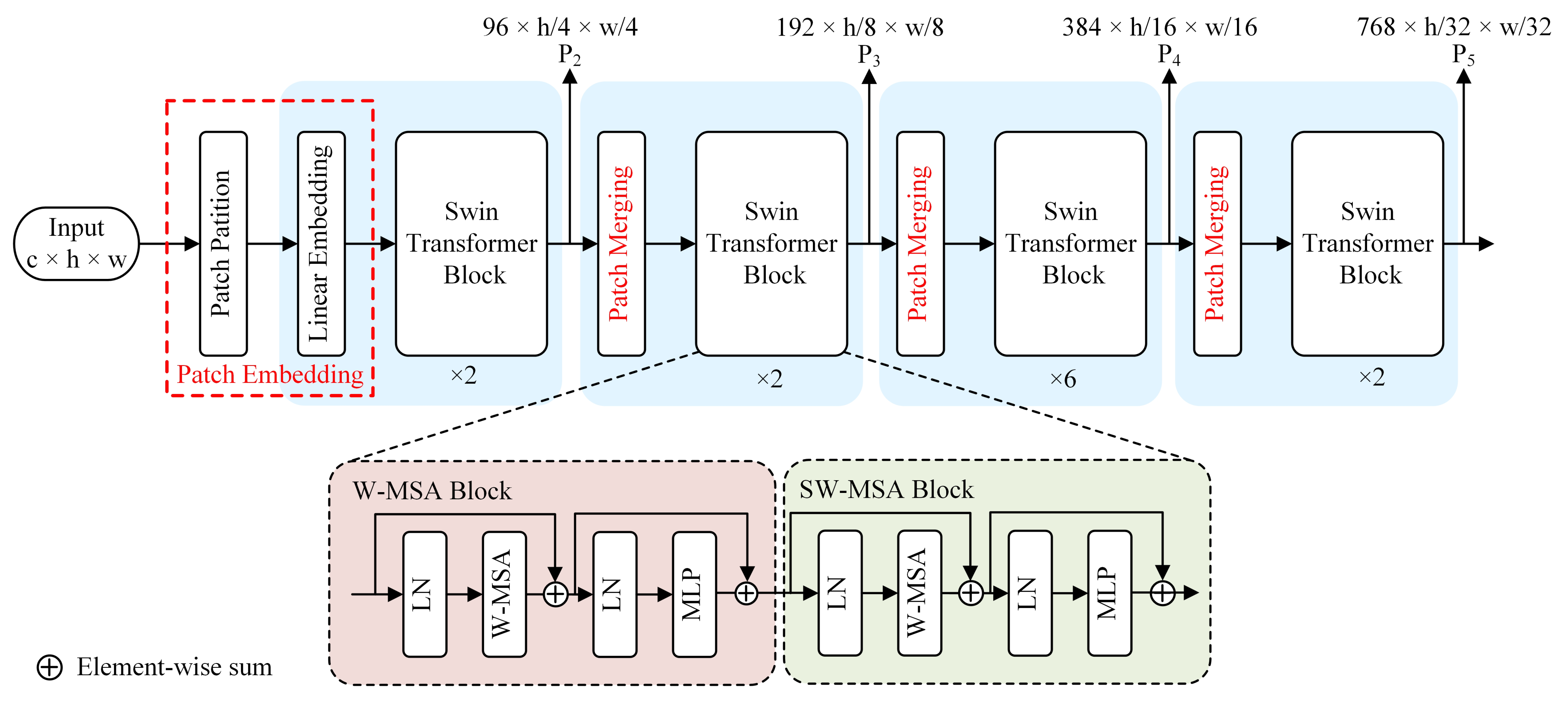
Swin Transformer [31] is an effective strategy for applying self-attention in computer vision, and has made the following improvements compared to previous work: (1) introducing the hierarchical construction method commonly used in CNN to build a hierarchical Transformer; (2) introducing the locality idea to perform self- attention calculation within the window region without overlap; (3) proposing a shifted window partitioning method to realize the window-based self-attention module connection. The computational complexity is linearly related to the input image size based on the above work. As depth increases, image blocks are gradually merged to construct a hierarchical Transformer, which can be used as a general-purpose visual backbone network.
The structure of the backbone network based on the Swin Transformer is shown in Figure 4. Patch embedding consists of patch partition and linear embedding layers; patch partition slices the feature-map module into small non-overlapping patches and linear embedding maps the input features into arbitrary dimensions. The Swin Transformer block consists of W-MSA (window multi-head self-attention) and SW-MSA (shifted-window multi-head self-attention). The W-MSA reduces the computational effort by dividing the feature map, and the SW-MSA enables information transfer between different windows. Patch merging downsamples the input feature map. Firstly, the original feature map of size c × h × w is input to the patch embedding module; the feature map is partitioned into small non-overlapping patches to build a 96 × (h/4) × (w/4) feature map, and then input to two successive stacked Swin Transformer block modules to obtain a 96 × (h/4) × (w/4) feature map. After that, through three patch merging layers and the Swin Transformer blocks, the feature maps , , and are obtained. , , are used as the input feature maps of the neck part of theFPN (feature pyramid networks) module. The structure of YOLOv5 using Swin Transformer as the backbone network is shown in Figure 5.
2.2.2. Improvement of Multi-Scale Feature Fusion
Compared with traditional handcrafted feature-based algorithms, the deep learning-based algorithms usually obtain low-level and high-level image features through convolutional neural networks and other feature extractors [32,33]. These features have different resolutions, so how to effectively process and fuse these multi-scale features has a critical impact on the networks that use them for inference. The feature pyramid network (FPN) [34] has performed pioneering work by using a top-down approach to combine multi-scale features. The path aggregation network (PANet) [35] further adds a bottom-up path to the FPN. The concrete approach is first to resize the feature maps to the same resolution and then add them up, in which features at different scales are treated equally. The neck of YOLOv5 also adopts the same approach to fuse features. Figure 6a shows the neck structure of YOLOv5 abstractly; assuming the input image size is 640 × 640, the PANet structure takes the features extracted by the backbone network with resolutions of 80 × 80, 40 × 40, and 20 × 20 at to levels, respectively, as input. As can be seen from the figure, FPN adopts a top-down approach, fusing the deep features with the underlying features by upsampling to obtain the predicted feature map. This operation conveys the strong semantic features from the upper layers downward, which enhances the learning ability of the model for image features, but some localization features might be lost. Therefore, PAN is added after FPN for its complementary effect with FPN by conveying strong localization features from the bottom up. Thus, the robustness and learning performance of the model is improved comprehensively. The process of aggregating multi-scale features can be expressed as:
where is the upsampling or downsampling operation and are the intermediate feature maps at level.
However, input features of different levels have different resolutions and they contribute variously to the output, so the network is required to take into account the importance of different feature layers by adding weights. To this end, we introduced learnable parameters as weights of different resolution features. The initial values were set to 1/m (m the number of different resolution features.) and optimized together with the model as parameters of the network. Furthermore, we also connected -level input features across layers, which can make the network more effective in aggregating multi-scale features without missing input features. The detailed structure of the network is shown in Figure 6b. The level output features are shown in Equation (4), which incorporates the weights of the different scale features and fuses the input features as well.
where is the upsampling operation, are the intermediate feature maps at level, and are weights.
2.2.3. Improvement of Confidence Loss Function Based on Detection Layers
The loss function, also called the cost function, maps the value of a random event or its associated random variable to a non-negative real number to represent the “risk” or “loss” of the random event. Neural networks generally use the method of minimizing the loss function to train the network so that it acquires excellent inference ability. The following three parts of the loss functions are utilized to optimize the YOLOv5 network. The first part is the loss that is caused by the prediction category , the second part is the loss that is due to the prediction frame positions x, y, h, w (upper left corner coordinates and aspect) , and the third part is the loss that comes from the confidence of the target , indicating the confidence rate with or without the target. The total loss function l was defined as:
Although YOLOv5 has excellent performance on the coco dataset, the accuracy of the network decreases when the materials change. Hence, the weights of the loss function should be adjusted according to the changes in the materials [36,37]. In our study, we found that despite YOLOv5 performing with high accuracy in our samples, the recall is not satisfactory, which implies that a large number of targets are not detected. Confidence represents the possibility of there being targets in the box or not. YOLOv5 calculates the confidence loss of different prediction heads respectively, then sums them in the same proportion as the total confidence loss, but different prediction heads are supposed to have different sensitivities to the targets. In this research, we adopt a new method based on IoU (Intersection over Union) to set the confidence loss of the detection layers.
IoU refers to the intersection-to-merge ratio, which calculates the ratio of intersection and merge between the predicted target frame and the true target frame, as shown in Equation (6).
where is the predicted frame and is the true frame. The network can be optimized by setting the weights of the confidence loss functions of different detection layers. The process of calculating the confidence loss function weights is shown in the flowchart in Figure 7. After each training epoch, the positive anchor box is calculated for each detection layer target. Among all the positive anchor boxes , the positive anchor box with IoU greater than the threshold (0.8× IoUmax) is obtained. Then, we calculate the change of compared to the previous epoch, denoted as △, and judge whether the percentage of the sum of △ relative to is less than the given threshold. When the value is less than the given threshold, the weights of the confidence loss function for each detection layer are calculated by Equation (7). Otherwise, the training is continued. Finally, the confidence loss function is set according to Equation (8).
where is the weight of the confidence loss function for detection layer i. is the balance factor. We found through experiments that there is a positive effect on the network when it is equal to 0.76. Through improving the confidence loss function, the sensitivity of different output layers to the targets is considered. The negative impact of low-quality anchor boxes on the model can be suppressed by this method, and the network will be biased to learn high-quality positive anchor boxes, which improves the capability of the network to capture the targets, thus increasing the recall.
3. Experiments
This section verifies the effectiveness and superiority of this paper’s improved algorithm in the underwater detection environment. The experimental results show that the improvement of the YOLOv5 target detection algorithm based on the methods in this paper can improve the accuracy of underwater target detection and make the algorithm more suitable for complex underwater environments.
3.1. Data Set
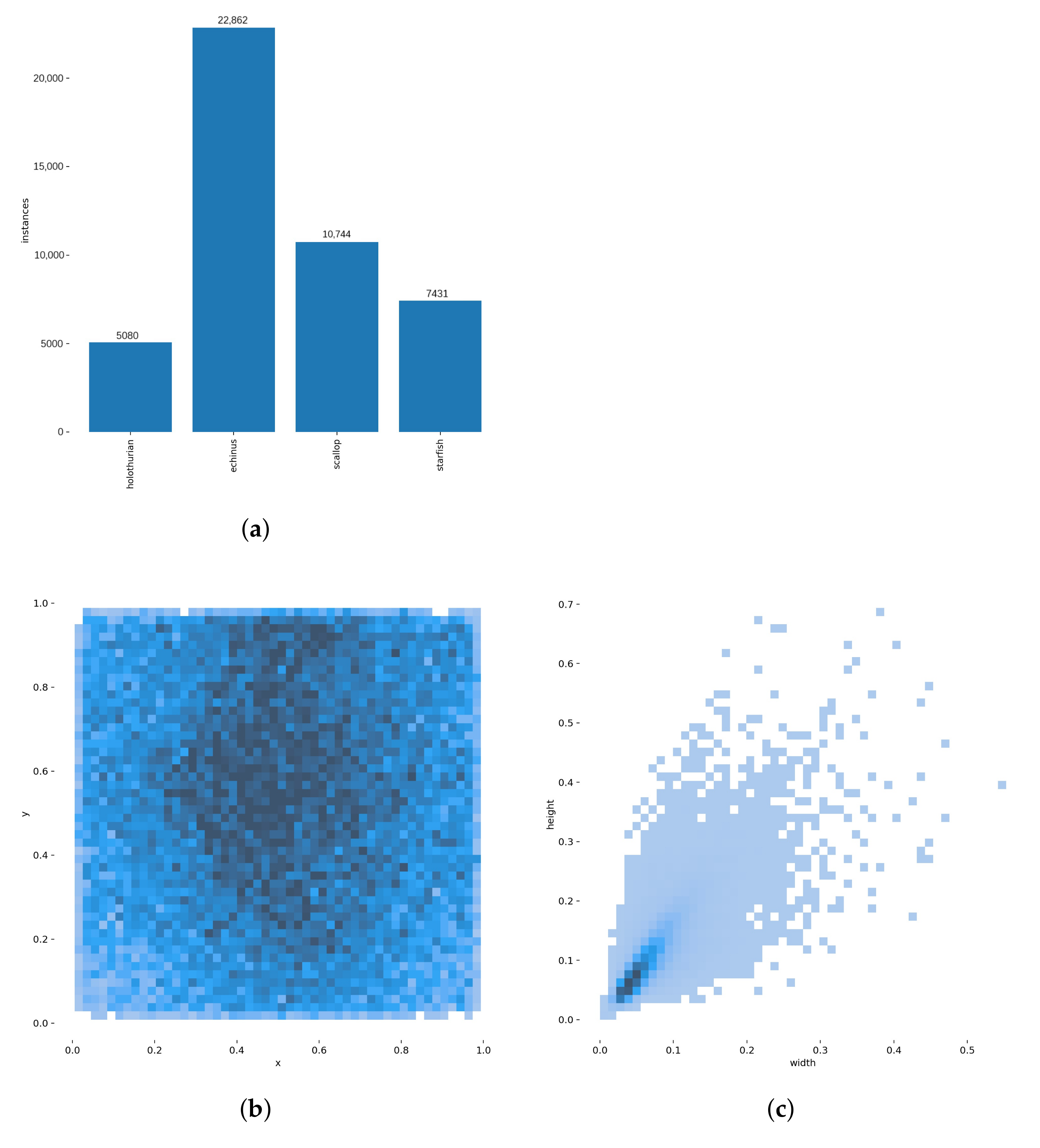
The experimental dataset is from the Target Recognition Group of China Underwater Robot Professional Competition (URPC), which contains underwater images of four different seafood species as shown in Figure 8, including “holothurian”, “echinus”, “scallop”, and “starfish”. We cleaned the data, removed the images that did not contain the detected targets, and retained 6034 valid images, then labeled the targets. All sample images were processed and stored according to the format of the PASAL VOC2007 sample set. Figure 9 shows the details of the dataset. Figure 9a shows the statistics of the number of targets in each class, in which echinus accounts for the majority, followed by scallop, starfish, and holothurian. Figure 9b is the normalized target location map, which is a right-angle coordinate system established by taking the lower left corner of the dataset image as the coordinate origin and using the relative coordinate values of the horizontal coordinate x and vertical coordinate y to evaluate the relative positions of the targets. The results show that the positions of the targets are spread throughout the coordinate system, are more concentrated in the horizontal direction, and are relatively dispersed in the vertical direction. Figure 9c is the normalized target size map. From the figure, we can see that the targets size distribution is relatively concentrated. The width is mainly distributed in 0∼0.1. The height is distributed in 0∼0.2. The targets are mostly small in size. To maintain the consistency of the data distribution, we randomly divided the dataset into a training set and a test set at a ratio of 7:3. The training set contains 4224 images and the test set contains 1810 images.
3.2. Model Evaluation Metrics
In target detection, representing these boxes as true targets or false targets can yield four potential predictions: true positive (TP), false positive (), true negative (), and false negative (). If the IoU between the detection box and the true box is greater than the threshold (it was set to 0.5 in our experiments), the detection box is marked as . Otherwise, it is marked as , and if there is no detection box matching the true box, it is marked as . represents the number of correctly identified targets, is the number of incorrectly identified targets, and is the number of targets that are not detected. The performance of the model can usually be evaluated by precision () and recall (), which are calculated by Equations (9) and (10).
Precision () and recall () are interactive. If the precision stays at a high value while the recall increases, it means that the model performs better. In contrast, a model with poorer performance may lose a significant amount of precision in exchange for improved recall. In order to combine the two metrics, average precision (AP) is introduced to measure the detection accuracy, as defined in Equation (11).
The value of AP is equal to the area under the precision-recall curve, and the higher the AP value, the higher the accuracy of the network. In the task of multi-class targets detection, the detection accuracy of the model is evaluated by calculating the average value of all types of AP (mAP), which is defined in Equation (12).
where C is the number of target categories.
3.3. Experimental Settings
We conducted experiments on an experimental platform equipped with an Intel(R) Xeon(R) Gold 5218 [email protected] GHz (192G RAM) and a NVIDIA GeForce RTX 3090 graphics processor (24 G RAM). The software environments were CUDA 10.1, CUDNN 7.6, and Python 3.7. The model was optimized by the SGD (stochastic gradient descent) method. The specific settings of hyperparameters of the network training are shown in Table 1. The training epochs were set to 500, the batch size was set to 16, the initial learning rate was set to 0.01, the weight decay was set to 0.0005, and the SGD momentum was set to 0.9. In addition, we also used the data enhancement technique in YOLOv5. The hyperparameters settings of data enhancement as shown in Table 2.
3.4. Experimental Results
YOLOv5 is divided into four different models based on the depth and width of the model: YOLOv5s, YOLOv5m, YOLOv5l, and YOLOv5x. The parameter settings are shown in Table 3, with an increasing Depth Multiple and Width Multiple, the number of model parameters and model size also increase linearly. YOLOv5s, as the lightest model, contains the least number of parameters and is convenient to deploy in realistic application scenarios. YOLOv5x contains the most parameters and the largest size, and is comparatively not easy to train. We conducted experiments based on different models. It can be seen from the table that the average AP (mAP) of the model improves as the depth and width of the model increase. There is 0.8% improvement between the largest model and the smallest model, but this also consumes a huge amount of computational resources. To reduce the consumption of computational resources, we selected YOLOv5s as a baseline for improvement and conducted further experiments.
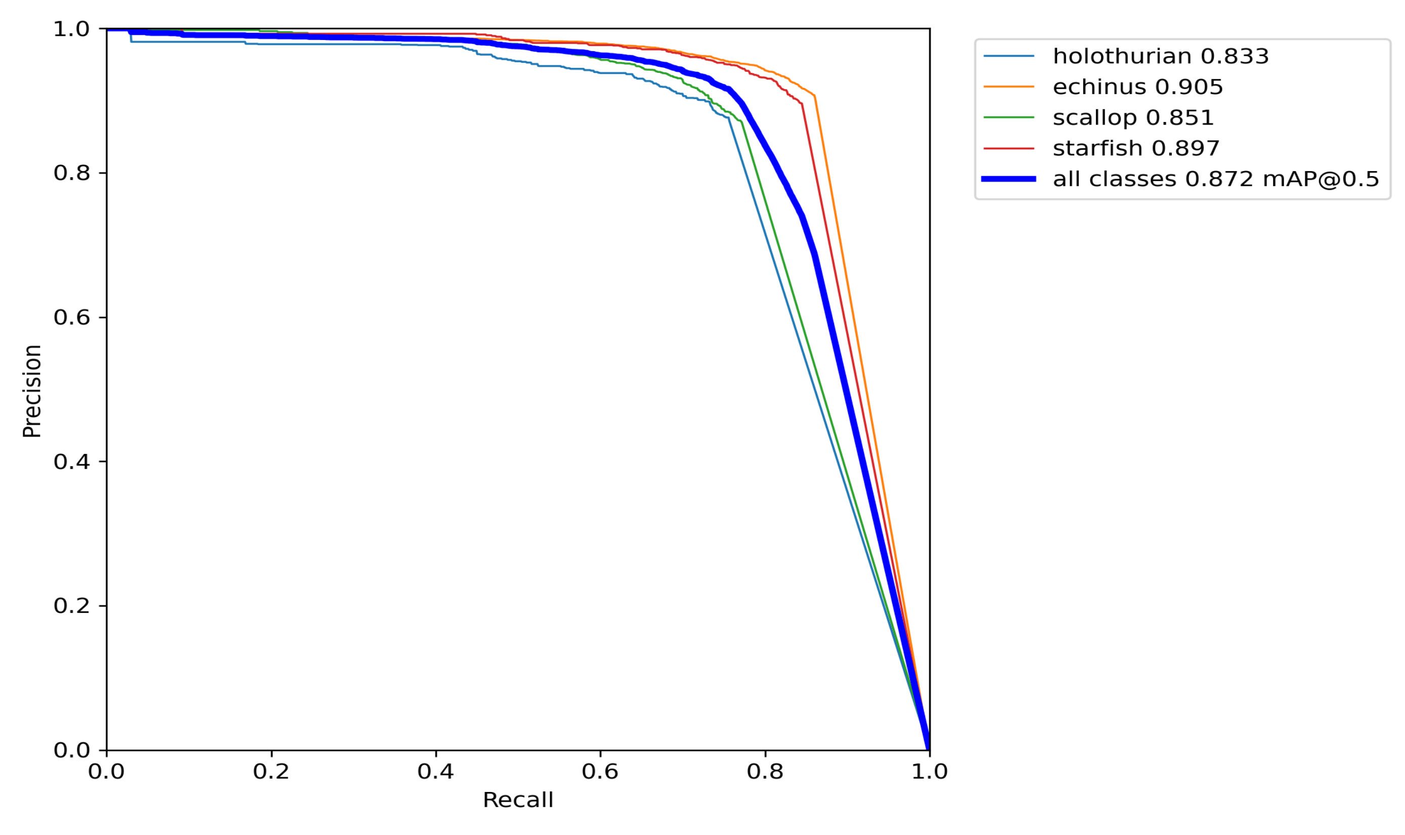
Figure 10 shows the precision-recall curve of the improved YOLOv5s model. It can be seen from the figure that the improved model achieves better detection results for all classes of targets; in particular, the AP value for echinus reaches 90.5%. The value of mAP is 87.2%
The confusion matrix is shown in Figure 11. The column indicates the predicted category and the row indicates the true category. The sum of the values in each column equals 1 and the value in each row indicates the proportion of predictions in the corresponding category. As can be seen from the figure, most of the targets were correctly predicted, which indicates that the model has good performance.
Figure 12 shows the variation curves of the loss values, including classification loss (Figure 12a), localization loss (Figure 12b), and confidence loss (Figure 12c). As can be seen from the figure, the different classes of losses steadily decrease as the number of iterations increases. The model converged after 100 iterations.
We conducted ablation experiments to intuitively observe the impact of different improvements on the model performance. As the anchor frame in the standard YOLOv5 algorithm is obtained based on the coco dataset, which is not suitable for our underwater dataset, we pre-set the anchor frame based on prior knowledge. Next, we used a redesigned backbone network based on Swin Transformer to extract features, then improved the PANet multi-scale fusion network, and finally improved the confidence loss function. The experimental results are shown in Table 4. Among them, using Swin Transformer as the backbone network of the model to obtain more useful features was the most critical improvement, as it improved the mAP of the model by 1.5%. The mAP of the network was improved by 0.3% by pre-setting the anchor frame in the initial stage of the experiment. Through the improvement of the multi-scale feature fusion method and the confidence loss function, the mAP was also improved by 0.2% and 0.3%, respectively.
To demonstrate the superiority of the improved method based on YOLOv5, YOLOv4 and SSD were used as other models for comparison experiments. The experimental results are shown in Table 5; compared with other models, the improved YOLOv5s model has the highest mAP. The mAP of the improved YOLOv5s model (87.2% mAP) exceeds SSD (60.9% mAP) by 26.3%, and is higher than YOLOv4 and standard YOLOv5s by 5.0% and 2.3%, respectively. It also significantly exceeded the largest model, YOLOv5x (85.7% mAP), by 1.5%. The experimental results indicate that the method is significantly superior for underwater target identification.
4. Discussion
Due to the shortcomings of convolutional neural (CNN) for target detection in harsh underwater scenes, we innovatively introduced Swin Transformer as the basic backbone network of YOLOv5 to highlight the target features, as well as improved the traditional PANet network and confidence loss function. Experimental results show that the improved model based on the method proposed in this study has excellent performance in harsh underwater scenes. As shown in Figure 13, the model works well for both single-class and multi-class targets in the case of blurred near and far images, and all targets in the images are detected accurately.
However, our model still suffers from false detections and missed detections when the environment is overly complex. Figure 14 shows examples of incorrect detection. In Figure 14a, the water weeds are incorrectly identified as holothurian. In Figure 14b, water weeds and stones are identified as echinus. We have put additional markers in the figures for incorrect recognitions. In Figure 14c,d, a large number of scallops were not detected.
Table 6 shows the training time, testing time, precision, and recall of the model. Our model was trained for 45 h and took 31 milliseconds to detect an image. The detection speed reached 32 FPS. The model size was 775 M. The precision and recall were 88.4% and 88.1%, respectively. We know from the above data that our model satisfies the real-time requirement with high precision and recall, but the model size is relatively large.
5. Conclusions
Underwater target detection algorithms have good performance on land at this phase, but are not suitable for complex underwater environments. In this paper, we proposed an underwater target detection algorithm based on the improved YOLOv5. The modified algorithm includes three key steps. Firstly, Swin Transformer was introduced as the basic backbone network of YOLOv5 to highlight the target features. Secondly, the multi-resolution feature fusion method was improved; the improved method can fuse images of different resolutions more effectively. Finally, the confidence loss function was improved to reduce the negative impact of low-quality anchor boxes on the network, so that the network can be biased to learn high-quality positive anchor boxes and improve its ability to detect targets. We compared the detection results of different models of YOLOv5 through experiments, conducted ablation experiments for the improved strategy, and conducted comparison experiments with other models. The experimental results show that the detection results of the YOLOv5 model in complex underwater environments were improved by the above improvements. The improved model outperforms the general target detection model and is more robust in complex underwater scenarios.
However, it is worth noting that our experiments were conducted only on one dataset, which may be limited in number and type because of the difficulty of collecting underwater datasets. It is also essential to use underwater image enhancement techniques for underwater datasets due to the poor quality of underwater images caused by the inability of light to completely transmit through water. In addition, the size of our model is relatively large. In our future research, we will collect datasets containing additional underwater target detection types and use image enhancement techniques in our models. Designing a lightweight network to speed up inference without losing accuracy will be another focus of future research.
Author Contributions
Data curation, F.T.; methodology, F.L.; project administration, F.L.; software, F.L.; supervision, S.L.; validation, F.T.; writing—original draft, F.L.; writing—review and editing, F.T. and S.L. All authors have read and agreed to the published version of the manuscript.
Funding
This research received no external funding.
Institutional Review Board Statement
Not applicable.
Informed Consent Statement
Not applicable.
Acknowledgments
We appreciate the comments from three anonymous reviewers which greatly improved the manuscript.
Conflicts of Interest
The authors declare no conflict of interest.
References
- Zeng, L.; Sun, B.; Zhu, D. Underwater target detection based on Faster R-CNN and adversarial occlusion network. Eng. Appl. Artif. Intell. 2021, 100, 104190. [Google Scholar] [CrossRef]
- Chen, L.; Zheng, M.; Duan, S.; Luo, W.; Yao, L. Underwater Target Recognition Based on Improved YOLOv4 Neural Network. Electronics 2021, 10, 1634. [Google Scholar] [CrossRef]
- Sahoo, A.; Dwivedy, S.K.; Robi, P. Advancements in the field of autonomous underwater vehicle. Ocean Eng. 2019, 181, 145–160. [Google Scholar] [CrossRef]
- Carlucho, I.; De Paula, M.; Wang, S.; Petillot, Y.; Acosta, G.G. Adaptive low-level control of autonomous underwater vehicles using deep reinforcement learning. Robot. Auton. Syst. 2018, 107, 71–86. [Google Scholar] [CrossRef] [Green Version]
- Forsyth, D. Object detection with discriminatively trained part-based models. Computer 2014, 47, 6–7. [Google Scholar] [CrossRef]
- Lowe, D.G. Distinctive image features from scale-invariant keypoints. Int. J. Comput. Vis. 2004, 60, 91–110. [Google Scholar] [CrossRef]
- Dalal, N.; Triggs, B. Histograms of oriented gradients for human detection. In Proceedings of the 2005 IEEE Computer Society Conference on Computer Vision and Pattern Recognition (CVPR’05), San Diego, CA, USA, 20–25 June 2005; Volume 1, pp. 886–893. [Google Scholar]
- Platt, J. Sequential minimal optimization: A fast algorithm for training support vector machines. Adv. Kernel Methods-Support Vector Learn. 1998, 208. Available online: https://www.microsoft.com/en-us/research/uploads/prod/1998/04/sequential-minimal-optimization.pdf (accessed on 1 January 2022).
- Shen, Z.; Liu, Z.; Li, J.; Jiang, Y.G.; Chen, Y.; Xue, X. Dsod: Learning deeply supervised object detectors from scratch. In Proceedings of the IEEE International Conference on Computer Vision, Venice, Italy, 22–29 October 2017; pp. 1919–1927. [Google Scholar] [CrossRef] [Green Version]
- Girshick, R.; Donahue, J.; Darrell, T.; Malik, J. Rich feature hierarchies for accurate object detection and semantic segmentation. In Proceedings of the IEEE Conference on Computer Vision and Pattern Recognition, Columbus, OH, USA, 23–28 June 2014; pp. 580–587. [Google Scholar] [CrossRef] [Green Version]
- Girshick, R. Fast r-cnn. In Proceedings of the IEEE International Conference on Computer Vision, Santiago, Chile, 7–13 December 2015; pp. 1440–1448. [Google Scholar]
- Ren, S.; He, K.; Girshick, R.; Sun, J. Faster R-CNN: Towards real-time object detection with region proposal networks. IEEE Trans. Pattern Anal. Mach. Intell. 2016, 39, 1137–1149. [Google Scholar] [CrossRef] [PubMed] [Green Version]
- Dai, J.; Li, Y.; He, K.; Sun, J. R-fcn: Object detection via region-based fully convolutional networks. In Proceedings of the Advances in Neural Information Processing Systems, Barcelona, Spain, 5–10 December 2016; pp. 379–387. [Google Scholar]
- He, K.; Gkioxari, G.; Dollár, P.; Girshick, R. Mask R-CNN. IEEE Trans. Pattern Anal. Mach. Intell. 2017, 42, 386–397. [Google Scholar] [CrossRef] [PubMed]
- Cai, Z.; Vasconcelos, N. Cascade r-cnn: Delving into high quality object detection. In Proceedings of the IEEE Conference on Computer Vision and Pattern Recognition, Salt Lake City, UT, USA, 18–23 June 2018; pp. 6154–6162. [Google Scholar]
- Liu, W.; Anguelov, D.; Erhan, D.; Szegedy, C.; Reed, S.; Fu, C.Y.; Berg, A.C. Ssd: Single shot multibox detector. In Proceedings of the European Conference on Computer Vision, Amsterdam, The Netherlands, 11–14 October 2016; pp. 21–37. [Google Scholar]
- Redmon, J.; Divvala, S.; Girshick, R.; Farhadi, A. You only look once: Unified, real-time object detection. In Proceedings of the IEEE Conference on Computer Vision and Pattern Recognition, Las Vegas, NV, USA, 27–30 June 2016; pp. 779–788. [Google Scholar]
- Redmon, J.; Farhadi, A. YOLO9000: Better, faster, stronger. In Proceedings of the IEEE Conference on Computer Vision and Pattern Recognition, Honolulu, HI, USA, 21–26 July 2017; pp. 7263–7271. [Google Scholar]
- Redmon, J.; Farhadi, A. Yolov3: An incremental improvement. arXiv 2018, arXiv:1804.02767. [Google Scholar]
- Bochkovskiy, A.; Wang, C.Y.; Liao, H.Y.M. Yolov4: Optimal speed and accuracy of object detection. arXiv 2020, arXiv:2004.10934. [Google Scholar]
- Villon, S.; Chaumont, M.; Subsol, G.; Villéger, S.; Claverie, T.; Mouillot, D. Coral reef fish detection and recognition in underwater videos by supervised machine learning: Comparison between Deep Learning and HOG+ SVM methods. In Proceedings of the International Conference on Advanced Concepts for Intelligent Vision Systems, Lecce, Italy, 24–27 October 2016; pp. 160–171. [Google Scholar]
- Li, X.; Shang, M.; Qin, H.; Chen, L. Fast accurate fish detection and recognition of underwater images with fast r-cnn. In Proceedings of the OCEANS 2015-MTS/IEEE Washington, Washington, DC, USA, 19–22 October 2015; pp. 1–5. [Google Scholar]
- Li, X.; Shang, M.; Hao, J.; Yang, Z. Accelerating fish detection and recognition by sharing CNNs with objectness learning. In Proceedings of the OCEANS 2016-Shanghai, Shanghai, China, 10–13 April 2016; pp. 1–5. [Google Scholar]
- Chen, L.; Zhou, F.; Wang, S.; Dong, J.; Li, N.; Ma, H.; Wang, X.; Zhou, H. SWIPENET: Object detection in noisy underwater images. arXiv 2020, arXiv:2010.10006. [Google Scholar]
- Lin, W.H.; Zhong, J.X.; Liu, S.; Li, T.; Li, G. Roimix: Proposal-fusion among multiple images for underwater object detection. In Proceedings of the ICASSP 2020-2020 IEEE International Conference on Acoustics, Speech and Signal Processing (ICASSP), Barcelona, Spain, 4–8 May 2020; pp. 2588–2592. [Google Scholar]
- Qiao, W.; Khishe, M.; Ravakhah, S. Underwater targets classification using local wavelet acoustic pattern and Multi-Layer Perceptron neural network optimized by modified Whale Optimization Algorithm. Ocean Eng. 2021, 219, 108415. [Google Scholar] [CrossRef]
- Wang, C.Y.; Liao, H.Y.M.; Wu, Y.H.; Chen, P.Y.; Hsieh, J.W.; Yeh, I.H. CSPNet: A new backbone that can enhance learning capability of CNN. In Proceedings of the IEEE/CVF Conference on Computer Vision and Pattern Recognition Workshops, Seattle, WA, USA, 14–19 June 2020; pp. 390–391. [Google Scholar]
- Vaswani, A.; Shazeer, N.; Parmar, N.; Uszkoreit, J.; Jones, L.; Gomez, A.N.; Kaiser, Ł.; Polosukhin, I. Attention is all you need. In Proceedings of the Advances in Neural Information Processing Systems, Long Beach, CA, USA, 4–9 December 2017; pp. 5998–6008. [Google Scholar]
- Dosovitskiy, A.; Beyer, L.; Kolesnikov, A.; Weissenborn, D.; Zhai, X.; Unterthiner, T.; Dehghani, M.; Minderer, M.; Heigold, G.; Gelly, S.; et al. An image is worth 16x16 words: Transformers for image recognition at scale. arXiv 2020, arXiv:2010.11929. [Google Scholar]
- Zhu, X.; Lyu, S.; Wang, X.; Zhao, Q. TPH-YOLOv5: Improved YOLOv5 Based on Transformer Prediction Head for Object Detection on Drone-captured Scenarios. In Proceedings of the IEEE/CVF International Conference on Computer Vision, Montreal, QC, Canada, 11–17 October 2021; pp. 2778–2788. [Google Scholar]
- Liu, Z.; Lin, Y.; Cao, Y.; Hu, H.; Wei, Y.; Zhang, Z.; Lin, S.; Guo, B. Swin transformer: Hierarchical vision transformer using shifted windows. arXiv 2021, arXiv:2103.14030. [Google Scholar]
- Ma, J.; Yuan, Y. Dimension reduction of image deep feature using PCA. J. Vis. Commun. Image Represent. 2019, 63, 102578. [Google Scholar] [CrossRef]
- Xiao, Y.; Tian, Z.; Yu, J.; Zhang, Y.; Liu, S.; Du, S.; Lan, X. A review of object detection based on deep learning. Multimed. Tools Appl. 2020, 79, 23729–23791. [Google Scholar] [CrossRef]
- Lin, T.Y.; Dollár, P.; Girshick, R.; He, K.; Hariharan, B.; Belongie, S. Feature pyramid networks for object detection. In Proceedings of the IEEE Conference on Computer Vision and Pattern Recognition, Honolulu, HI, USA, 21–26 July 2017; pp. 2117–2125. [Google Scholar]
- Liu, S.; Qi, L.; Qin, H.; Shi, J.; Jia, J. Path aggregation network for instance segmentation. In Proceedings of the IEEE Conference on Computer Vision and Pattern Recognition, Salt Lake City, UT, USA, 18–22 June 2018; pp. 8759–8768. [Google Scholar]
- Kendall, A.; Gal, Y.; Cipolla, R. Multi-task learning using uncertainty to weigh losses for scene geometry and semantics. In Proceedings of the IEEE Conference on Computer Vision and Pattern Recognition, Salt Lake City, UT, USA, 18–22 June 2018; pp. 7482–7491. [Google Scholar]
- Cai, Q.; Pan, Y.; Wang, Y.; Liu, J.; Yao, T.; Mei, T. Learning a unified sample weighting network for object detection. In Proceedings of the IEEE/CVF Conference on Computer Vision and Pattern Recognition, Seattle, WA, USA, 14–19 June 2020; pp. 14173–14182. [Google Scholar]
Figure 1.
The network structure of YOLOv5, which is composed of the input module, backbone network, neck network, and prediction network.
Figure 1.
The network structure of YOLOv5, which is composed of the input module, backbone network, neck network, and prediction network.

Figure 2.
Focus module slicing operation.

Figure 3.
The improved YOLOv5 is used for underwater target detection.

Figure 4.
The Swin Transformer architecture.

Figure 5.
The structure of YOLOv5 using Swin Transformer as the backbone network.

Figure 6.
(a) The structure of PANet; (b) the structure of the improved PANet.

Figure 7.
Flow chart of calculation of the confidence loss function weights.

Figure 8.
The dataset contains four biological categories, which are (a) holothurian, (b) echinus, (c) scallop, and (d) starfish.
Figure 8.
The dataset contains four biological categories, which are (a) holothurian, (b) echinus, (c) scallop, and (d) starfish.

Figure 9.
Statistical results of the dataset: (a) bar chart of the number of targets in each class; (b) normalized target location map; (c) normalized target size map.
Figure 9.
Statistical results of the dataset: (a) bar chart of the number of targets in each class; (b) normalized target location map; (c) normalized target size map.

Figure 10.
The precision-recall curve of the improved YOLOv5s.

Figure 11.
The confusion matrix of the improved YOLOv5s.

Figure 12.
The variation curves of the loss values: (a) classification loss; (b) localization loss; (c) confidence loss.
Figure 12.
The variation curves of the loss values: (a) classification loss; (b) localization loss; (c) confidence loss.

Figure 13.
Single-class and multi-class target detection results in the case of blurred images at close and far distances, where different color squares represent different targets, the red squares represent holothurian, the pink squares represent echinus, the yellow squares represent starfish: (a) single-class of targets at close range; (b) multi-class of targets at close range; (c) single-class of targets at far range; (d) multi-class of targets at far range.

Figure 14.
Examples of incorrect detection, where different color squares represent different targets, the red squares represent holothurian, the pink squares represent echinus, the yellow squares represent starfish, the orange squares represent scallop: (a,b) examples of incorrect detection; (c,d) examples of not detected.


Table 1.
Hyperparameter settings of network training.
| Training Epochs | Batch Size | Learning Rate | Weight Decay | Momentum |
|---|---|---|---|---|
| 500 | 16 | 0.01 | 0.0005 | 0.9 |
Table 2.
Hyperparameter settings of data enhancement.
| Translate (Image Translation) | Scale (Image Scale) | Fliplr (Image Flip Left-Right) | Flipud (Image Flip Up-Down) | Mosaic | Mixup |
|---|---|---|---|---|---|
| 0.1 | 0.5 | 0.1 | 0.5 | 1.0 | 0.1 |
Table 3.
Experimental results of different YOLOv5 models.
| Model | Depth Multiple | Width Multiple | Number of Parameters | Size of Model (MB) | mAP (%) |
|---|---|---|---|---|---|
| YOLOv5s | 0.33 | 0.50 | 14.1 | 84.9 | |
| YOLOv5m | 0.67 | 0.75 | 40.5 | 85.2 | |
| YOLOv5l | 1.0 | 1.0 | 89.4 | 85.6 | |
| YOLOv5x | 1.33 | 1.33 | 167.0 | 85.7 |
Table 4.
Ablation experiments.
| Pre-Set Anchor | Swin Transformer | Improved Multi-Scale Feature Fusion | Improved Confidence Loss Function | mAP (%) |
|---|---|---|---|---|
| 84.9 | ||||
| ✓ | 85.2 (+0.3) | |||
| ✓ | ✓ | 86.7 (+1.5) | ||
| ✓ | ✓ | ✓ | 86.9 (+0.2) | |
| ✓ | ✓ | ✓ | ✓ | 87.2 (+0.3) |
Table 5.
Experimental results of different algorithms.
| Method | Backbone Network | mAP (%) | AP (%, Holothurian) | AP (%, Echinus) | AP (%, Scallop) | AP (%, Starfish) |
|---|---|---|---|---|---|---|
| SSD | VGG-16 | 60.9 | 59.5 | 73.8 | 41.1 | 69.1 |
| YOLOv4 | Darknet-53 | 82.2 | 71.8 | 89.6 | 82.3 | 85.2 |
| YOLOv5s | CSPDarknet53 | 84.9 | 74.9 | 91.0 | 85.1 | 88.4 |
| YOLOv5x | CSPDarknet53 | 85.7 | 76.5 | 91.4 | 86.1 | 88.6 |
| Improved YOLOv5s | Swin Transformer | 87.2 | 83.3 | 90.5 | 85.1 | 89.7 |
Table 6.
Other indicators of improved YOLOv5s.
| Training Time (h) | Time Spent in Detection (ms) | Detection Speed (FPS) | Size of Model (MB) | Precision (%) | Recall (%) |
|---|---|---|---|---|---|
| 45 | 31 | 32 | 775 | 88.4 | 81.1 |
Publisher’s Note: MDPI stays neutral with regard to jurisdictional claims in published maps and institutional affiliations. |
© 2022 by the authors. Licensee MDPI, Basel, Switzerland. This article is an open access article distributed under the terms and conditions of the Creative Commons Attribution (CC BY) license (https://creativecommons.org/licenses/by/4.0/).
Share and Cite
MDPI and ACS Style
Lei, F.; Tang, F.; Li, S. Underwater Target Detection Algorithm Based on Improved YOLOv5. J. Mar. Sci. Eng. 2022, 10, 310. https://doi.org/10.3390/jmse10030310
AMA Style
Lei F, Tang F, Li S. Underwater Target Detection Algorithm Based on Improved YOLOv5. Journal of Marine Science and Engineering. 2022; 10(3):310. https://doi.org/10.3390/jmse10030310
Chicago/Turabian StyleLei, Fei, Feifei Tang, and Shuhan Li. 2022. "Underwater Target Detection Algorithm Based on Improved YOLOv5" Journal of Marine Science and Engineering 10, no. 3: 310. https://doi.org/10.3390/jmse10030310
Note that from the first issue of 2016, this journal uses article numbers instead of page numbers. See further details here.