1. Introduction
The classical genetic model states that humans have two copies of each gene, one on each chromosome. The sequencing of individual human genomes, however, has revealed that there is an unexpected amount of structural variation present in our genetic makeup. Sections of DNA can be deleted or duplicated, leaving individuals with fewer or more copies of portions of their genome (such individuals are said to have a
CNV, or copy-number variation, at that position). Understanding the contribution of CNVs to human variation is one of the most compelling current challenges in genetics [
1].
As the coverage of single nucleotide polymorphism (SNP) arrays has increased, it is increasingly possible to use this data to infer the CNV status of individuals. Indeed, recent generations of such chips include probes specifically designed to enable measurement of copy number [
2,
3]. Although other technologies for determining copy number exist, the use of genotyping chips has a clear advantage in that hundreds of genome-wide association studies have been performed [
4], and these studies may be mined for CNV data at no added cost. Many of these studies have been carried out with very large sample sizes, thereby enabling CNV studies on a scale that would otherwise be prohibitively expensive [
5,
6]. These factors have led to a number of studies using data from high-density genotyping arrays to investigate the nature of copy-number variation and its role in human variation and disease [
7,
8,
9,
10,
11].
Two general strategies have been proposed for conducting genetic association studies of copy-number variation. The majority of analytic techniques attempt to (1) identify or “call” CNVs for each individual, then (2) carry out association tests of whether individuals with a CNV differ from individuals without a CNV with regard to disease or some other phenotype. An alternative approach is to reverse the order of those two steps: (1) carry out association testing at the single marker level, then (2) aggregate information from neighboring markers to determine CNVs associated with disease/phenotype. The key idea of both approaches is that, because the data is noisy, it is virtually impossible to identify CNV associations from a single marker. Because copy number variants extend over multiple markers in a sufficiently high-density array, however, we are able to carry out inferences regarding CNVs by pooling information across neighboring markers.
We refer to these two approaches, respectively, as
variant-level testing and
marker-level testing. In Breheny
et al. [
12], the authors explored the relative strengths and weaknesses of the two approaches and reached the conclusion that marker-level approaches were better able to identify associations involving small, common CNVs, while variant-level approaches were better able to identify associations involving large, rare CNVs.
One serious complication with variant-level testing is that the estimated CNV boundaries from different individuals do not, in general, coincide. This presents a number of difficulties. Whether or not two individuals with partially overlapping CNVs should be in the same risk group for the purposes of association testing is ambiguous and complicates both the association test itself, as well as attempts to correct for multiple comparisons. With a large sample size, the complexity of partially overlapping CNV patterns quickly becomes daunting. Marker-level testing is an attractive alternative, as the aggregation is carried out on the test results, thereby avoiding the complications posed by partially overlapping CNV call boundaries during the analysis process.
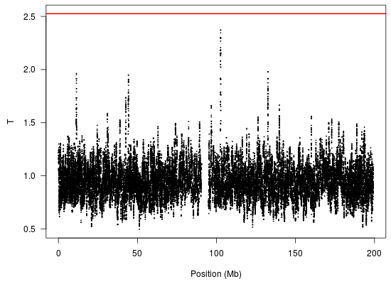
We illustrate the idea behind marker-level testing and aggregation in
Figure 1, which plots a negative log transformation of the
p-values of the marker-level tests
vs. position along the chromosome. The details of the hypothesis tests for this example are described in
Section 4, but the
p-values may arise from any test for association between copy number intensity [
13] and phenotype. The salient feature of the plot is the cluster of small
p-values between 102.5 and 102.7 Mb. The presence of so many low
p-values in close proximity to one another suggests an association between the phenotype and copy-number variation in that region.
Figure 1.
Illustration of marker-level testing. The values from the marker-level tests are plotted as a function of position along the chromosome.
Figure 1.
Illustration of marker-level testing. The values from the marker-level tests are plotted as a function of position along the chromosome.
To locate these clusters on a genome-wide scale, Breheny
et al. [
12] used a marker-level approach based on circular binary segmentation [
14,
15]. Here, we take a closer look at the problem of aggregating
p-values from marker-level tests. We present two main findings. First, we develop a computationally efficient kernel-based approach for
p-value aggregation. Second, we analyze the multiple comparison properties of this approach and of
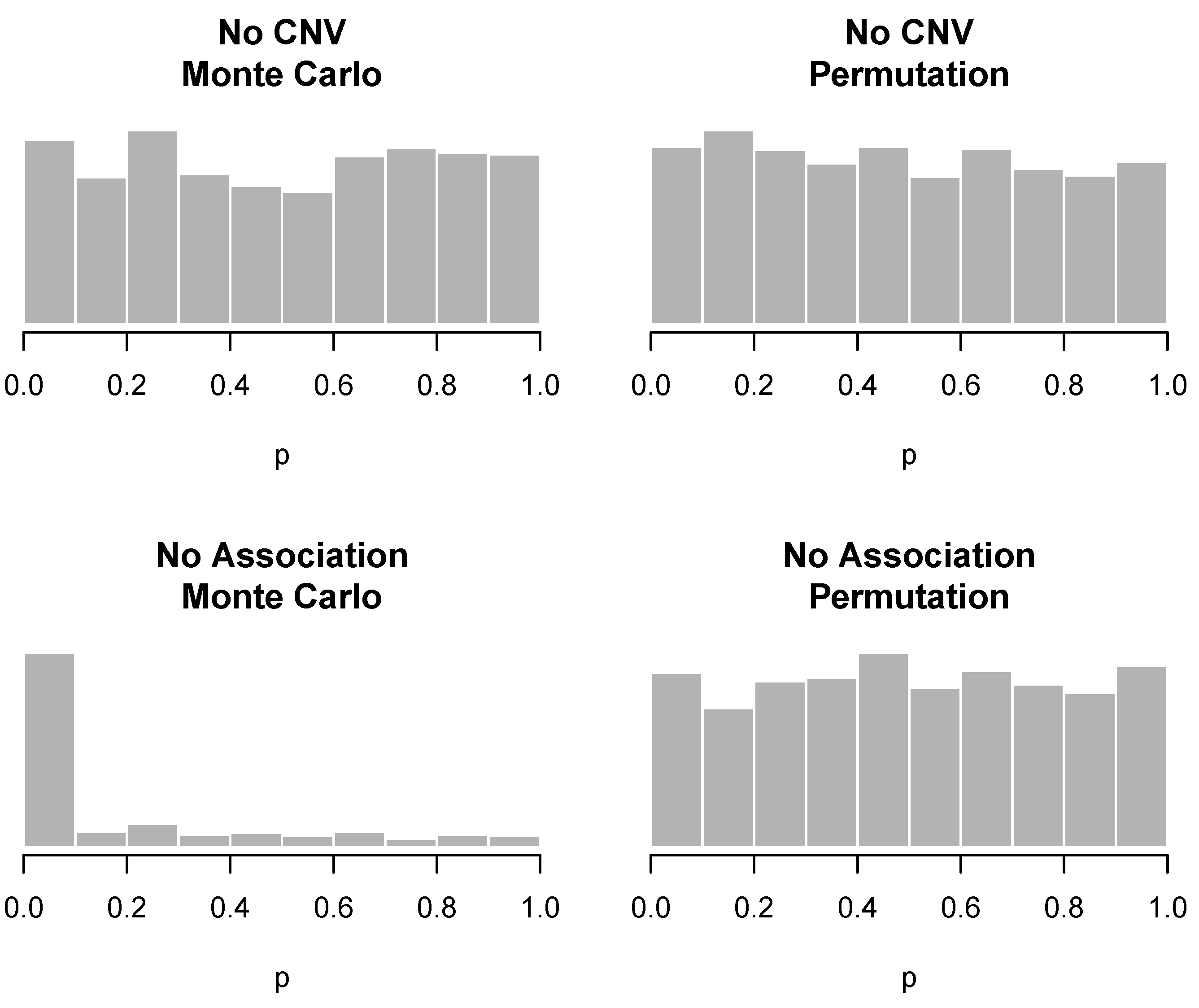
p-value aggregation in general. In particular, we demonstrate that naïve aggregation approaches assuming exchangeability of test statistics do not preserve the family-wise error rate (FWER). To solve this problem, we present a permutation-based approach and show that it preserves family-wise error rates while maintaining competitive power.
2. Kernel-Based Aggregation
Throughout, we will use i to index subjects and j to index markers. Let denote the intensity measurement for subject i at marker j, let denote the phenotype for subject i and let denote the p-value arising from a test of association between phenotype and intensity at marker j. Finally, let denote the location of marker j along the chromosome and J denote the total number of markers; in this article, we use physical distance, but genetic distance could be used instead.
Consider the aggregation
where
is a function of the test results for marker
j and
is a kernel that assigns a weight to
depending on how far away marker
j is along the chromosome from the target location,
. The parameter
h defines the bandwidth of the kernel and, thereby, controls the bias-variance tradeoff—a larger bandwidth pools test results over a larger region and, thereby decreases variance, but potentially introduces bias by mixing test results beyond the boundary of a CNV with those inside the boundary.
Although, in principle, one could apply Equation (
1) at any arbitrary location
, we restrict attention here to locations at which a marker is present and for which the bandwidth does not extend beyond the borders of the chromosome, thereby obtaining a finite set of aggregates
. We will consider transformations
such that low
p-values lead to large values of
, leading to significance testing at the aggregate level based on the statistic
.
In this section, we describe the choice of kernel and transformation , as well as the issue of incorporating the direction of association for signed tests.
2.1. Choice of Kernel
We consider two primary choices with regard to the kernel: shape and definition of bandwidth. First, we may consider varying the shape of the kernel. Two common choices are the flat (“boxcar”) kernel and the Epanechnikov kernel:
Intuitively, the Epanechnikov kernel would seem more attractive, as it gives higher weight to markers near the target location and diminished weight to distant markers where bias is a larger concern.
Besides varying the shape of the kernel, we consider two definitions of bandwidth, which we refer to as
constant width and
constant marker (these concepts are sometimes referred to as “metric” and “adaptive” bandwidths, respectively, in the kernel smoothing literature). In the constant width approach, as illustrated in Equations (
2) and (
3), the width,
h, of the kernel is constant.
In contrast, the constant marker approach expands and contracts the range of the kernel as needed, so that there are always
k markers in the positive support of the kernel. Specifically, the constant marker approach replaces the scalar
h in Equations (
2) and (
3) with the function
, where
is the location of the
kth closest marker to
x. For the constant width approach, the number of markers given positive weight by the kernel varies depending on
.
The general tradeoff between the two approaches is that as we vary the target location,
, constant width kernels suffer from fluctuating variance, because the effective sample size is not constant, whereas constant marker kernels suffer from fluctuating bias, because the size of the region over which test results are pooled is not constant. We investigate the benefits and drawbacks of these various kernels in
Section 5.
As a point of reference, the flat, constant marker kernel is similar to the simple moving average, although not exactly the same. For example, consider the following illustration.
Suppose . At , the three nearest neighbors are , while at , the three nearest neighbors are . Thus, combinations such as are not considered by the kernel approach. This prevents the method from aggregating test results over inappropriately disperse regions of the chromosome, such as across the centromere.
2.2. Transformations
Directly pooling
p-values is not necessarily optimal. Various transformations of
p may be able to better discriminate true associations from noise. Specifically, we consider the following transformations:
where the text to the left of the equation is the label with which we will refer to these transformations in later figures and tables. The transformations are constructed in such a way that low
p-values produce high values of
for all three transformations.
All three transformations have a long history in the field of combining
p-values. Forming a combination test statistic based on the sum of
values (or equivalently, the log of the product of the
p-values) was first proposed by Fisher [
16]—the so-called Fisher combination test. The transformation (
5) was proposed by Stouffer
et al. [
17], who also studied the properties of sums of these normal-transformed
p-values. Finally, Equation (
4) was proposed and studied by Edgington [
18]. The theoretical properties of these proposals have since been studied by several authors [
19,
20,
21,
22]. Throughout this literature, the majority of work has focused on these scales—uniform, Gaussian and logarithmic—each of which has been shown to have advantages and drawbacks. There is no uniformly most powerful method of combining
p-values [
23].
The present application differs from the classical work described above in that the borders of the CNVs are not known. Thus, we do not know the appropriate set of
p-values to combine. Consequently, we must calculate many combinations,
, which are partially overlapping and, therefore, not independent, thereby requiring further methodological extensions. The implications of these concerns are addressed in
Section 3.
2.3. Direction of Association
Some association tests (
z-tests,
t-tests) have a direction associated with them, while others (
-tests,
F-tests) do not. As we will see in
Section 5, it is advantageous to incorporate this direction into the analysis when it is available, as it diminishes noise and improves detection. We introduce here extensions of the transformations presented in
Section 2.2 that include the direction of association.
Let denote the direction of association for test j. For example, in a case control study, if intensities were higher for cases than controls at marker j, then . At markers where CNV intensities were higher for controls than cases, . The signs are arbitrary; their purpose is to reflect the fact that an underlying, latent CNV affects both phenotype and intensity measures; thus, switching directions of association are inconsistent with the biological mechanism being studied and likely to be noise.
When
is available, we adapt the three transformations from
Section 2.2 as follows:
All of these transformations have the same effect: when and , ; when and , ; and when , , regardless of the value of . In other words, the test results combine to give an aggregate value, , that is large in absolute value only if the test results have low p-values and are consistently in the same direction.
4. Gemcitabine Study
In this section, we describe a pharmacogenomic study of gemcitabine, a commonly used treatment for pancreatic cancer. We begin by describing the design of the study (this description is similar to that provided in [
12]), then analyze data from the study using the proposed kernel-based aggregation method. This data will also be used to simulate measurement errors for the simulation studies in
Section 5.
The gemcitabine study was carried out on the Human Variation Panel, a model system consisting of cell lines derived from Caucasian, African-American and Han Chinese-American subjects (Coriell Institute, Camden, NJ, USA). Gemcitabine cytotoxicity assays were performed at eight drug dosages (1,000, 100, 10, 1, 0.1, 0.01, 0.001 and 0.0001 uM) [
24]. Estimation of the phenotype IC
(the effective dose that kills 50% of the cells) was then completed using a four parameter logistic model [
25]. Marker intensity data for the cell lines was collected using the Illumina HumanHap 550K and HumanHap 510S at the Genotyping Shared Resources at the Mayo Clinic in Rochester, MN, which consists of a total of 1,055,048 markers [
26,
27]. Raw data were normalized according to the procedure outlined in Barnes
et al. [
5].
172 cell lines (60 Caucasian, 53 African-American and 59 Han Chinese-American) had both gemcitabine cytotoxicity measurements and genome-wide marker intensity data. To illustrate the application of the kernel-based aggregation approach, we selected one chromosome (chromosome 3) from the genome-wide data. To control for the possibility of population stratification, which can lead to spurious associations, we used the method developed by Price
et al. [
28], which uses a principal components analysis (PCA) to adjust for stratification. At each marker, a linear regression model was fit with PCA-adjusted IC
as the outcome and intensity at that marker as the explanatory variable; these models produce the marker-level tests.
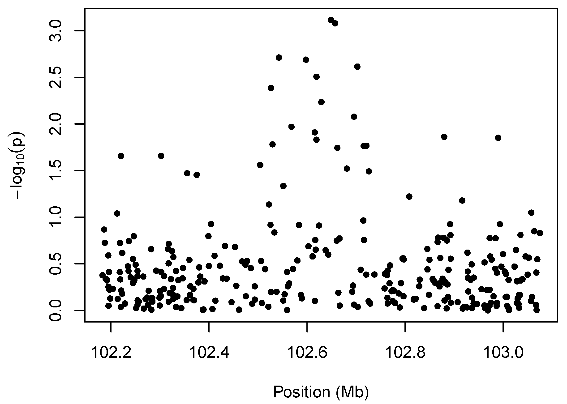
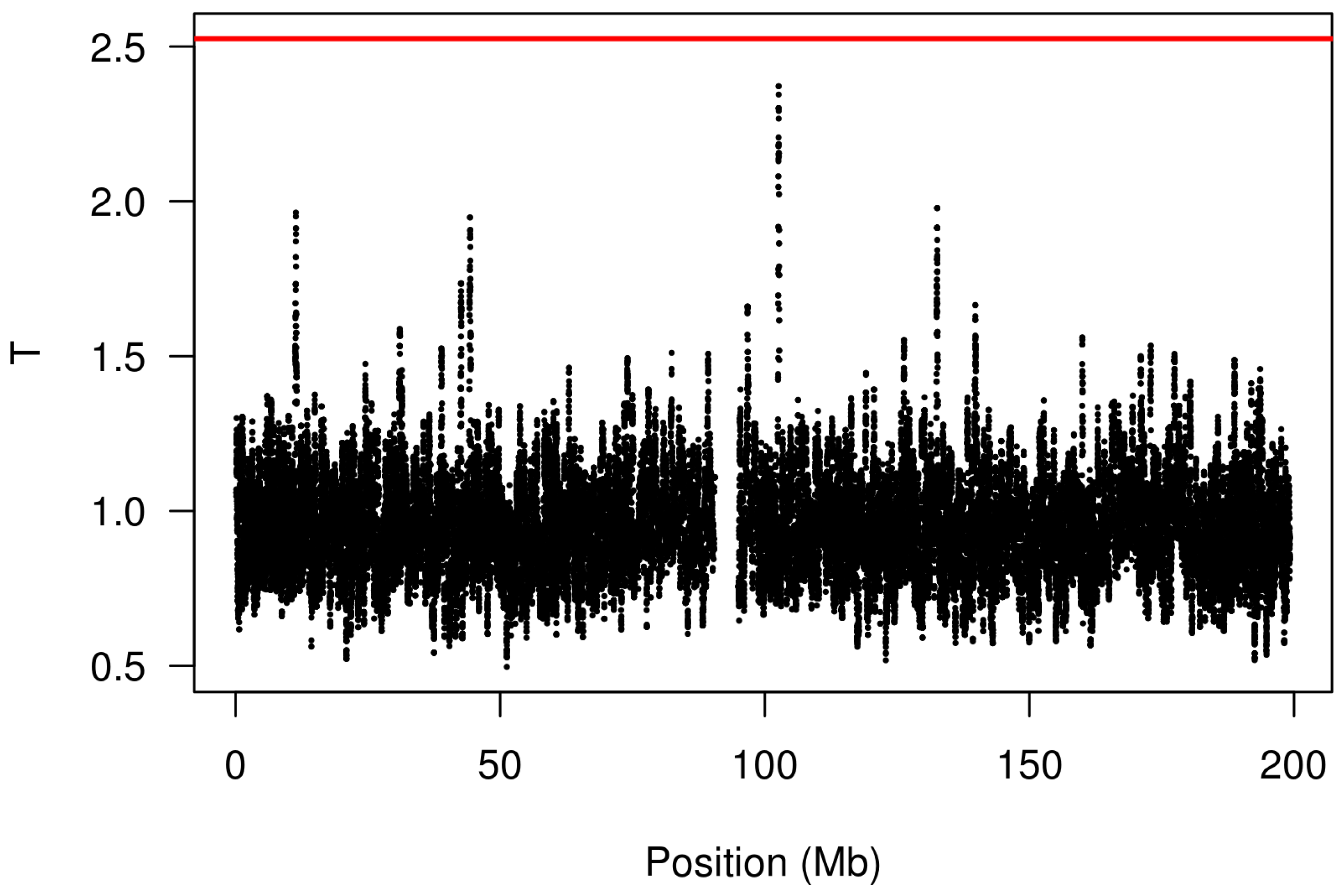
We analyzed these data using the kernel-based approach described in
Section 2 with a bandwidth of 50 markers and the log transformation. The results are shown in
Figure 3. Note the presence of a peak at 102.6 Mb; this genomic region was also illustrated in
Figure 1. The red line indicates the FWER-controlled, chromosome-wide significance threshold at the
level. As the figure indicates, there is insufficient evidence in this study to establish a CNV association involving response to gemcitabine (
p = 0.16) after controlling the chromosome-wide FWER. Other choices of bandwidth and transformation produce qualitatively similar, although somewhat less significant, results.
Copy number variation in the region of chromosome 3 at 102.6 Mb, which is in close proximity to the gene, ZPLD1, has been found by Glessner
et al. [
29] to be associated with childhood obesity. An earlier analysis of this data by Breheny
et al. [
12] indicated suggestive evidence that this region harbors a CNV association with gemcitabine response, but lacked a formal way to control the error rate at the chromosome-wide level. This example illustrates the need for the more rigorous approach we develop here. The lack of significance in this example is perhaps not surprising, in that 172 subjects is a relatively small sample size for a CNV association study.
Figure 3.
Analysis of the gemcitabine data (chromosome 3) using the proposed kernel aggregation method. The kernel aggregations, , are plotted against chromosomal position. The red line indicates the cutoff for chromosome-wide FWER significance at the level.
Figure 3.
Analysis of the gemcitabine data (chromosome 3) using the proposed kernel aggregation method. The kernel aggregations, , are plotted against chromosomal position. The red line indicates the cutoff for chromosome-wide FWER significance at the level.
5. Simulations
5.1. Design of Spike-in Simulations
In this section, we study the ability of the proposed approach to detect CNV-phenotype associations using simulated CNVs and corresponding intensity measurements. The validity of our conclusions depends on how realistic the simulated data is, so we have given careful thought to simulating this data in as realistic a manner as possible. The spike-in design that we describe here is also described in Breheny
et al. [
12].
The basic design of our simulations is to use real data from the gemcitabine study described in
Section 4, “spike” a signal into it, then observe the frequency with which we can recover that signal. We used circular binary segmentation [
14,
15] to estimate each sample’s underlying mean intensity at every position along the chromosome, then subtracted the actual intensity measurement from the estimated mean to obtain a matrix of residuals representing measurement error. This matrix, denoted
, has 172 rows (one for each subject) and 70,542 columns (one for each marker).
We then used these residuals to simulate noise over short genomic regions in which a single simulated CNV is either present or absent. Letting i denote subjects and j denote markers, the following variables are generated: , an indicator for the presence or absence of a CNV in individual i; , the intensity measurement at marker j for individual i; and , the phenotype. For the sake of clarity, we focus here on a random sampling design in which the outcome is continuous; similar results were obtained from a case-control sampling design in which the outcome is binary. In the random sampling design, the CNV indicator, , is generated from a Bernoulli distribution where is the frequency of the CNV in the population; subsequently, is generated from a normal distribution whose mean depends on .
For each simulated data set, 200 markers were independently selected at random from the columns of . The measurement error for simulated subject i was then drawn from the observed measurement errors at those markers for a randomly chosen row of . Thus, within a simulated data set, all subjects are studied with respect to the same genetic markers, but the markers vary from data set to data set. Simulating the data in this way preserves all the features of outliers, heavy-tailed distributions, skewness, unequal variability among markers and unequal variability among subjects that are present in real data.
The intensity measurements,
, derive from these randomly sampled residuals. To the noise, we add a signal that depends on the presence of the simulated CNV
. The added signal is equal to zero unless the simulated genome contains a CNV encompassing the
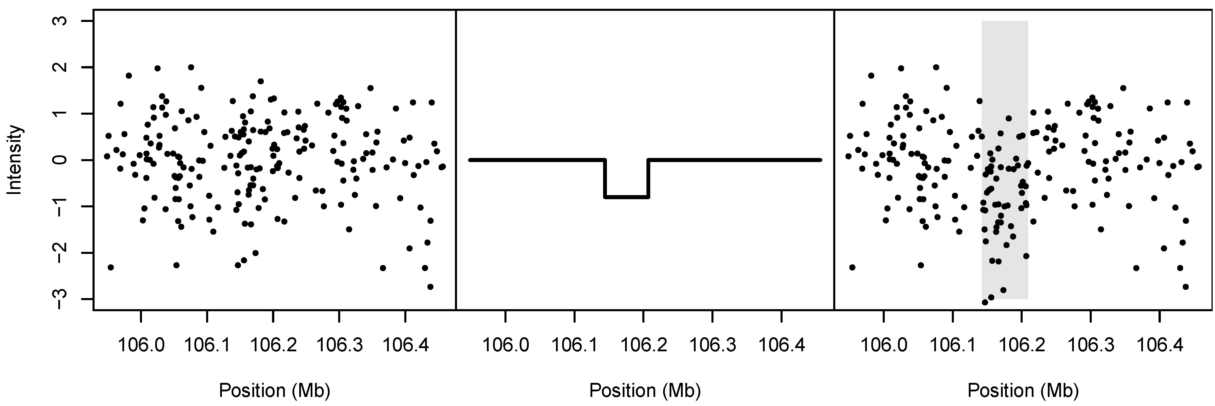
jth marker; otherwise, the added signal is equal to the standard deviation of the measurement error times the signal-to-noise ratio. Our simulations employed a signal-to-noise ratio of 0.8, which corresponded roughly to a medium-sized detectable signal based on our inspection of the gemcitabine data. Note that the phenotype and intensity measurement are conditionally independent given the latent copy-number status
. An illustration of the spike-in process is given in
Figure 4.
For the Illumina Human1M-Duo BeadChip, which has a median spacing of 1.5 kb between markers, 200 markers corresponds to simulating a 300 kb genomic region. We varied the length of the CNV from 10 to 50 markers, corresponding to a size range of 15 to 75 kb. For the simulations presented in the remainder of the article, we used a sample size of and an effect size (change in mean divided by standard deviation) for the continuous outcome of 0.4.
Figure 4.
Illustration of spike-in simulation design. Left: The noise, randomly drawn from among the estimated measurement errors for a single cell line. Middle: The spiked-in signal. Right: The resulting simulated data; the gray shaded region denotes the boundary of the spiked-in CNV.
Figure 4.
Illustration of spike-in simulation design. Left: The noise, randomly drawn from among the estimated measurement errors for a single cell line. Middle: The spiked-in signal. Right: The resulting simulated data; the gray shaded region denotes the boundary of the spiked-in CNV.
5.2. Transformations
We begin by examining the impact on power of the various transformations proposed in
Section 2.2 and
Section 2.3. In order to isolate the effect of transformation, we focus here on the “optimal bandwidth” results: the bandwidth of the kernel was chosen to match the number of markers in the underlying CNV. This will lead to the maximum power to detect a CNV-phenotype association, although this approach is clearly not feasible in practice, as the size of an underlying CNV is unknown.
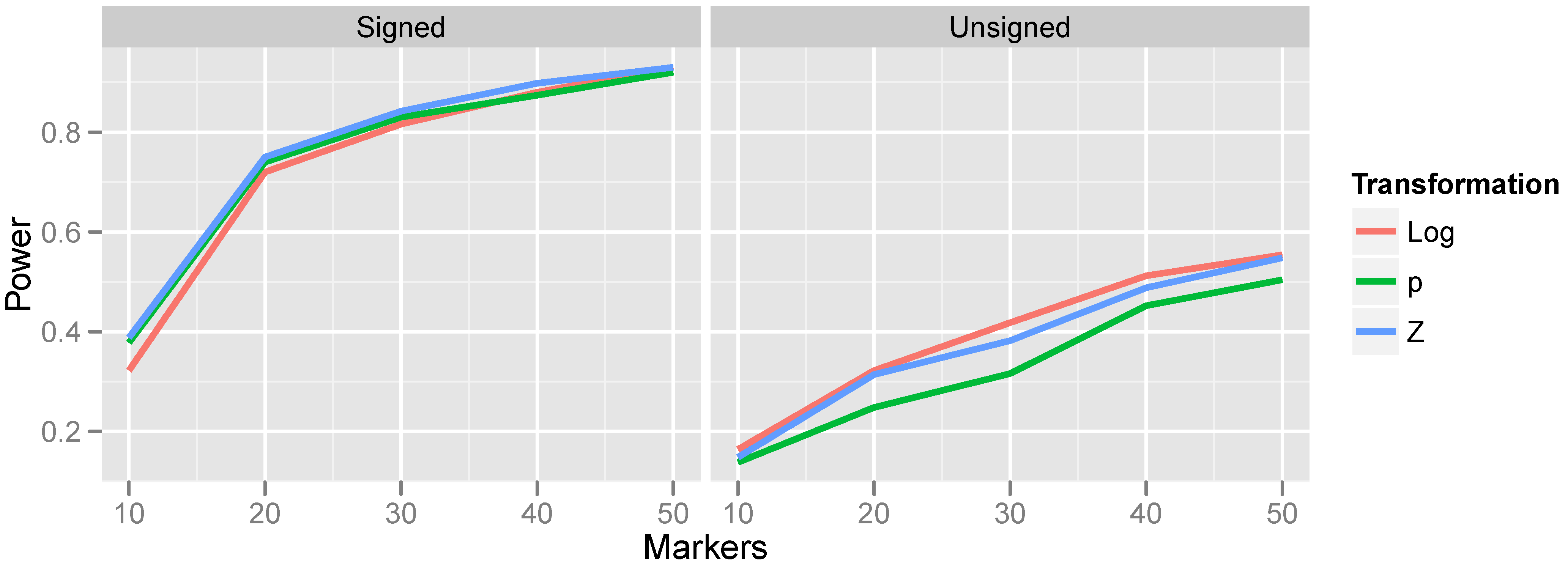
Figure 5.
Effect of transformation choice on power. Population CNV frequency was set to 10%; optimal bandwidths were used. Lines are colored according to the transformations, which were defined in Equations (
4)–(
9).
Figure 5.
Effect of transformation choice on power. Population CNV frequency was set to 10%; optimal bandwidths were used. Lines are colored according to the transformations, which were defined in Equations (
4)–(
9).
The relationship between power and transformation choice is illustrated in
Figure 5. The figure illustrates a basic trend that held consistently over many CNV frequencies and bandwidth choices: although the various transformations do not dramatically alter power, the normalizing transformation (Z) is most powerful for signed test results, while the log transformation is most powerful for unsigned test results. In the results that follow, unless otherwise specified, we employ the normalizing transformation for signed test results and the log transformation for unsigned tests. The substantial gain in power attained by incorporating the direction of association is also apparent from
Figure 5 by comparing the left and right halves of the figure.
5.3. Choice of Kernel
In this section, we examine two aspects of kernel choice: bandwidth implementation (constant-width
vs. constant-marker) and kernel shape (flat
vs. Epanechnikov), defined in
Section 2.1. When all markers are equally spaced, the constant-width and constant-marker kernels are equivalent. To examine the impact on power when markers are unequally spaced, we selected at random a 200-marker sequence from chromosome 3 of the combined set of markers Illumina HumanHap 550K and 510S genotyping chips and spiked in CNVs of various sizes. The optimal bandwidth (either in terms of the number of markers or base pairs spanned by the underlying CNV) was chosen for each method.
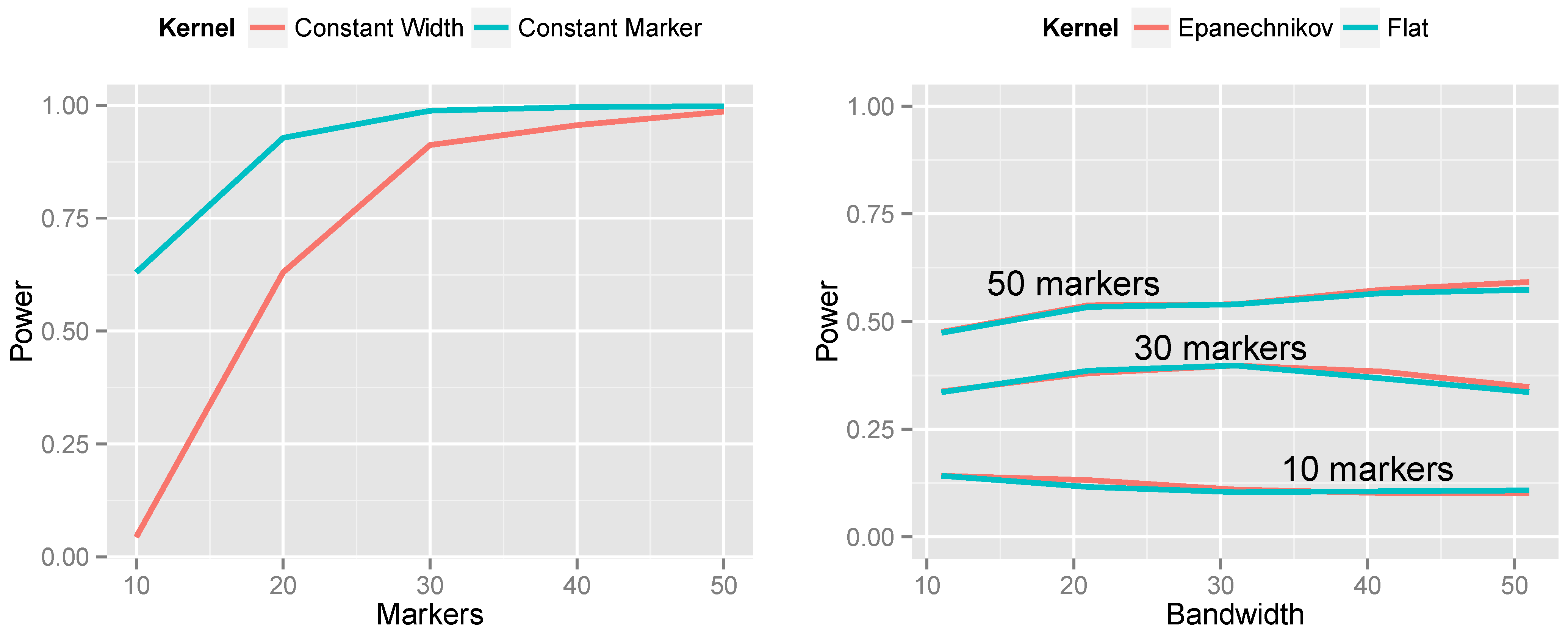
The left side of
Figure 6 presents the results of this simulation. The constant-marker approach is substantially more powerful. When the number of markers is not held constant, the aggregation measure
is more highly variable for some values of
j than others. This causes the null distribution of
to have thicker tails, which, in turn, increases the
p-value for the observed
, thus lowering power. This phenomenon manifests itself most dramatically for small bandwidths. Consequently, throughout the rest of this article, we employ constant-marker kernels for all analyses.
Figure 6.
Effect of kernel choice on power. Left: Constant-width kernel vs. constant-marker kernel. Right: Flat vs. Epanechnikov kernel. In both plots, population CNV frequency was 10%, test results were unsigned and the log transformation was used.
Figure 6.
Effect of kernel choice on power. Left: Constant-width kernel vs. constant-marker kernel. Right: Flat vs. Epanechnikov kernel. In both plots, population CNV frequency was 10%, test results were unsigned and the log transformation was used.
The right side of
Figure 6 presents the results of changing the kernel shape from the flat kernel described in Equation (
2) to the Epanechnikov kernel described in Equation (
3). We make several observations: (1) the shape of the kernel has little impact on power; the two lines are nearly superimposed. (2) The kernel approach is relatively robust to choice of bandwidth; even five-fold differences between the bandwidth and optimal bandwidth do not dramatically decrease power. (3) Nevertheless, the optimal bandwidth does indeed occur when the number of markers included in the kernel matches the true number of markers spanned by the CNV. And (4), the Epanechnikov kernel is slightly more robust to choosing a bandwidth that is too large than the flat kernel is. This makes sense, as the Epanechnikov kernel gives less weight to the periphery of the kernel.
5.4. Kernel-Based Aggregation vs. Variant-Level Testing
Lastly, we compare the kernel-based aggregation approach with variant-level testing. To implement variant-level testing, each sample was assigned a group (“variant present” or “variant absent”) on the basis of whether a CNV was detected by CBS. A two-sample
t-test was then carried out to test for association of the CNV with the phenotype. This variant-level approach was compared with kernel-based aggregation of marker-level testing for a variety of bandwidths. The results are presented in
Figure 7.
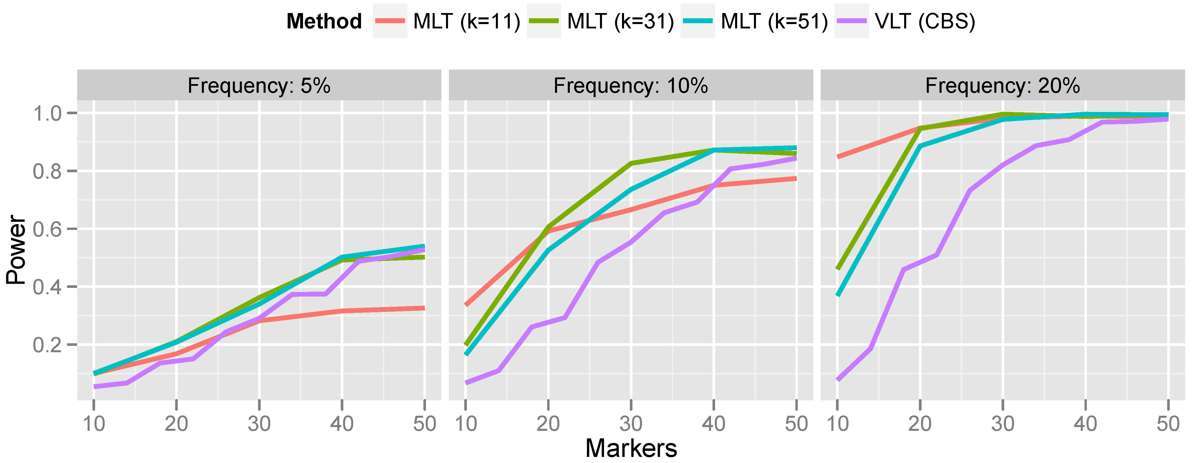
For rare CNVs (5% population frequency), the power of the variant-level approach and the aggregated marker-level approach are comparable. However, for more common CNVs, the marker-level approach offers a substantial increase in power. For the most part, this increase in power persists even when the bandwidth is misspecified. Only when the bandwidth was much too small (selecting a 10-marker bandwidth for a 50-marker CNV) did the variant-level approach surpass marker-level aggregation.
Generally speaking, these results are consistent with the findings reported in Breheny
et al. [
12], who found that variant-level tests have optimal power relative to marker-level tests when CNVs are large and rare; conversely, marker-level tests have optimal power relative to variant-level tests when CNVs are small and common. This is understandable, given the limited accuracy of calling algorithms for small CNVs.
Comparing the results in
Figure 7 with the results of Breheny
et al. [
12], who aggregated marker-level tests by applying CBS to the
p-values, as described in
Section 3.1, we find that the kernel approach is a substantially more powerful method for aggregating marker-level tests than the change-point testing carried out by CBS. Specifically, Breheny
et al. found that the change-point approach had very low power at 5% frequency—much lower than the variant-level approach. On the other hand, in the same setting, we find that the kernel approach is comparable to, and even slightly more powerful than, the variant-level approach. Furthermore, as discussed in
Section 3.1, a change-point analysis of marker-level tests also relies on exchangeability, which does not always hold. Thus, the methods developed in this article are both more powerful and achieve better control over the FWER than the CBS change-point analysis described in Breheny
et al. [
12].
Figure 7.
Power comparison of variant-level testing (using CBS for CNV calling) with marker-level testing (using kernel-based aggregation). For the marker aggregation, k is the bandwidth (number of markers included in the kernel).
Figure 7.
Power comparison of variant-level testing (using CBS for CNV calling) with marker-level testing (using kernel-based aggregation). For the marker aggregation, k is the bandwidth (number of markers included in the kernel).
A potential drawback of the kernel approach is the need to specify a bandwidth. This makes the robustness of the method to bandwidth misspecification, as illustrated in
Figure 7, particularly important, because in practice, it is difficult to correctly specify the bandwidth
a priori. Indeed, it is possible that multiple CNVs associated with the outcome are present on the same chromosome and have different lengths. A method that is not robust to bandwidth will be incapable of detecting both CNVs. Generally speaking, a bandwidth of roughly 30 markers seems to provide good power over the range of CNV sizes that we investigate here.
6. Discussion
We have explored the use of a kernel-based method for aggregating tests that possess a spatial aspect, whereby underlying latent features cause nearby tests to be correlated, demonstrated some of the analytical challenges and developed an approach that properly accounts for multiple comparisons in a challenging setting. Our motivation for this work is the problem of association testing involving copy-number variants, but our findings may also be applied to other problems in genome-wide association studies, such as testing for haplotype associations.
The computational burden of the method is worth further discussion, due to the permutation testing requirement. For simple tests, such as the linear regression tests we used in the gemcitabine study, the burden is quite manageable. On our machine (using an Intel Xeon 3.6 GHz processor), it took under a second to perform the 70,542 marker-level tests on chromosome 3 and under 0.1 s to perform the kernel aggregation. Carrying out 1,000 permutation tests took 1,000 times longer: 15 min to carry out all the permutation tests and 21 s to perform all the kernel aggregation. Extrapolating, a genome-wide analysis would take 3.5 h.
These calculations, however, are for simple marker-level tests and a fairly small sample size (
). Larger studies will increase the computation burden linearly (
i.e., doubling the subjects should double the computing time), but more complicated marker-level tests based on nonlinear, mixed-effects or mixture models would require substantially more time. Fortunately, the procedure is easy to run in parallel on multiple cores or machines, with each processor carrying out a fraction of the permutation tests. It is also worth pointing out that kernel aggregation may be used as an exploratory tool without the need for permutation testing (the black dots of
Figure 3 may be calculated rapidly; the red line is what requires the permutation testing). Nevertheless, ongoing research in our group is focusing on ways to speed up the approach described here with a model-based formulation that avoids the need for permutation testing.
The simulation studies of
Section 5 address a limited-scale version of a larger question: how do marker-level test aggregation and variant-level testing compare for chromosome-wide and genome-wide analysis? This is an important question and deserves further study. In general, multiplicity is a thorny issue for CNV analyses, as the true locations of CNVs are unknown and can overlap in a number of complicated ways. The issue of how many tests to carry out and adjust for is a challenging question for variant-level testing and a considerable practical difficulty in analysis. In contrast, aggregation of marker-level results avoids this issue altogether. We have shown that the proposed approach is both powerful at detecting CNV associations and rigorously controls the FWER at a genome-wide level—two appealing properties. However, future work analyzing additional studies using kernel aggregation and studying its properties in larger, more complex settings is necessary.


