Automated Classification of the Tympanic Membrane Using a Convolutional Neural Network


Department of Otorhinolaryngology-Head and Neck Surgery, Asan Medical Center, University of Ulsan College of Medicine, 88, Olympic-ro 43-gil, Songpa-gu, Seoul 05505, Korea
*
Authors to whom correspondence should be addressed.
Appl. Sci. 2019, 9(9), 1827; https://doi.org/10.3390/app9091827
Submission received: 1 March 2019
/
Revised: 24 March 2019
/
Accepted: 28 April 2019
/
Published: 2 May 2019
(This article belongs to the Section Applied Biosciences and Bioengineering)
Abstract
:Precise evaluation of the tympanic membrane (TM) is required for accurate diagnosis of middle ear diseases. However, making an accurate assessment is sometimes difficult. Artificial intelligence is often employed for image processing, especially for performing high level analysis such as image classification, segmentation and matching. In particular, convolutional neural networks (CNNs) are increasingly used in medical image recognition. This study demonstrates the usefulness and reliability of CNNs in recognizing the side and perforation of TMs in medical images. CNN was constructed with typically six layers. After random assignment of the available images to the training, validation and test sets, training was performed. The accuracy of the CNN model was consequently evaluated using a new dataset. A class activation map (CAM) was used to evaluate feature extraction. The CNN model accuracy of detecting the TM side in the test dataset was 97.9%, whereas that of detecting the presence of perforation was 91.0%. The side of the TM and the presence of a perforation affect the activation sites. The results show that CNNs can be a useful tool for classifying TM lesions and identifying TM sides. Further research is required to consider real-time analysis and to improve classification accuracy.
1. Introduction
Middle ear diseases are diagnosed using patient’s history and otoscopic findings in the tympanic membrane (TM). Guidelines on otitis media highlight the usefulness of TM findings in diagnosing various types of otitis media [1]. The development of video endoscopes has enabled more accurate detection of diagnostic lesions. However, clinical diagnosis of otitis media is mainly subjective. In addition, it shows limited reproducibility due to the high reliance on the clinician experience and cooperation of the patients [2].
Artificial intelligence is often employed to perform high-level image analysis such as image classification, segmentation and matching. The success of such an analysis highly depends on feature extraction, for which deep learning is widely used [3]. In particular, convolutional neural networks (CNNs) have demonstrated good performance in automatic classification of medical images (e.g., skin lesions [4,5], eye lesions [6,7,8], radiologic and MRI images [9,10,11]). Several studies have applied deep learning for making diagnoses based on otoscopic images. Accuracies from 73.11% to 91.41% have been reported when applying deep learning to distinguish acute otitis media (AOM) and otitis media with effusion (OME) [12,13,14]. At the same time, chronic otitis media (COM) is challenging due to variability of the images and difficulty of locating lesions. Shie et al. proposed a machine-learning algorithm to classify normal middle ear, AOM, OME and COM with an accuracy of 88.06% [15].
In this study, we propose a machine-learning method to detect the TM findings accurately. The aim of the study is to build and evaluate a CNN model for TM classification (i.e., detecting TM side and presence or absence of perforation). The usefulness and reliability of the CNN in classifying TMs is also investigated.
2. Materials and Methods
2.1. Datasets
Following the approval of the Institutional Review Board (2018-0655) of the Asian Medical Center (AMC), we retrospectively reviewed images of TMs captured via an endoscopic system. TM images were collected at the Department of Otorhinolaryngology-Head & Neck Surgery in AMC between April 2016 and April 2018. All images were evaluated and categorized by two otologists (JYL and JWC). In this study, postoperative, retraction, attic lesion and inadequate images were excluded. A total of 1338 images were used for training; 714 (right: 347; left: 367) normal TMs and 624 (right: 305; left: 319) TMs with perforation. After the training phase, the model was applied to a new image set (right normal: 663; left normal: 773; right TM with perforation: 181; left TM with perforation: 201).
2.2. Deep Neural Network Model
The CNN model for detecting the TM side and presence of perforation was built using Python programming language. The model comprises six layers (Figure 1). The convolutional layers contain 32 masks. The kernel size is 3 × 3 in all convolutional layers and 2 × 2 in all max-pooling layers. The fully connected layer includes 128 nodes, whereas the last layer has only two nodes presented as output probabilities. The available images were randomly assigned to training, validation and testing sets in the ratio of 60%:20%:20%, respectively. Regarding the detailed hyperparameters used in this study, we tried a lot of combinations of hyperparameters to optimize CNN training and finally used hyperparameters are as follows: batch size 32, number of epochs 400, SGD as an optimizer, learning rate 0.0001, momentum 0.9, Nesterov momentum. Training dataset was augmented with sheer range 0.2, rotation range 5, horizontal flip for normal vs. perforation training.
The CNN was trained in the following two stages: first, to distinguish the TM side regardless of the lesion presence; second, to detect the presence of perforations (Figure 2). In the test phase, a class activation map (CAM) was applied to evaluate feature extraction. This process can effectively visualize feature variations in illumination, normal structures and lesions, which are commonly observed in images. The activation site was divided into eight parts as follows: external auditory canal, TM, tympanic annulus, malleolar short process, malleolar handle, umbo, cone of light, perforation margin and middle ear (Figure 3). The TM and external auditory canal (EAC) were divided into four subparts (anterior-posterior and superior-inferior). The CAM results were analyzed statistically using the Statistical Package for the Social Sciences (SPSS) software, version 22.0 (SPSS Inc., Chicago, IL, USA). Logistic regression was used to evaluate the statistical significance and odds ratio (OR).
3. Results
3.1. Accuracy
The classification accuracy was calculated as the number of correctly classified instances divided by the total number of considered instances and multiplied by 100. In the training phase, the accuracy of the CNN model was 98.7% for the TM side classification and 87.20% for the detection of perforation presence or absence. In the test phase, the accuracy of detecting the side of the normal TM was 99.2% for the right side and 96.5% for the left side. The accuracy of detecting the side of the TM with perforation was 99.5% for the right side and 95.6% for the left side. The accuracy of detecting presence or absence of perforation was 94.5% for the right side and 91.2% for the left side. The accuracy of finding no perforation was 91.7% for the right normal TM and 89.1% for the left normal TM. The accuracy of detecting perforation was 94.5% for the right TM with perforation and 91.2% for the left TM with perforation. The overall accuracy of the model was 98.7% for detecting the side and 91% for detecting the presence or absence of perforation (Table 1). Table 2 show the performance of the CNN model. The sensitivity and specificity of the model were 97.9% and 96.3% in the detection of side. In the detection of perforation, the sensitivity and specificity were 91.0% and 90.5%. The positive predictive value (PPV) and negative predictive value (NPV) were 96.9% and 99.1% for the detection of side and 98.0% and 72.3% for the detection of perforation.
3.2. Class Activation Map
The presence or absence of the heat map of the CAM image was calculated using a new dataset (right TM: 844; left TM: 974) of the test phase. The overall activation rate of the CAM was 8.7% for the left normal TM and 52.5% for the right normal TM. The overall analysis results are summarized in Table 3. The top three activation sites were the EAC anterior-inferior portion (52.2%), cone of light (46.1%) and malleolar short process (45.2%) in the left normal TM. For the side detection of the left normal TM, TM posterior-superior (OR: 17.56) and TM posterior-inferior (OR: 37.87) were statistically significant. However, there is no statistically significant subsite for the presence or absence of perforation. For the right normal TM, malleolar short process (89.9%), EAC posterior-superior (87.4%) and EAC anterior-inferior (86.8%) were frequent activation sites. There is no statistically significant site for the side detection and the detection of presence or absence of perforation. The overall activation rate for the TMs with perforation was 94.8% for the left and 60.3% for the right. EAC posterior-superior (74.3%), EAC posterior-inferior (63.3%) and middle ear (61.8%) were the top three activation sites for the left TM with perforation. Perforation margin (OR: 9.03) and middle ear (OR: 3.55) were statistically significant only in the detection of presence or absence of perforation for the left TM with perforation. For the right TM with perforation, middle ear (75.9%) was first, EAC anterior-inferior (59.8%) was second and perforation margin (53.9%) was third. For the right TM with perforation, middle ear (OR: 37.88) was statistically significant in the detection of the presence or absence of perforation. There was no statistically significant site in the detection of the side for the TM with perforation.
4. Discussion
Accurate diagnosis of the ear diseases requires mastery of the otoscopic examination [1]. Interpretation of the TM requires extensive training and experience with an associated learning curve [16]. It has been reported that pediatricians and otolaryngologists provide an accurate diagnosis of middle ear pathology in only 50% and 73% cases, respectively [17]. Some studies reported a diagnostic accuracy among otologists of 72–82% [18,19].
In some studies, diagnostic systems for AOM and OME rely on selected features used for image processing of otoscopic images. A diagnosis support system analyzing the color of the TM has been reported to achieve an accuracy of 73.11% [13]. Another diagnostic system using features that mimic an otologist’s decision-making process for otitis media has been reported to achieve an accuracy of 89.9% [14], while an automated feature extraction and classification system for AOM and OME has achieved an accuracy of 91.41% [12].
While many studies on AOM and OME have demonstrated excellent results, image classification studies on COM are rare since COM can show variable lesions and anatomical distortion, making feature selection more complicated. Shie et al. reported a computer-aided diagnostic system for otitis media [15]. They classified otitis media into four categories (normal, AOM, OME and COM) and the accuracy was 88.06%. The authors used different types of filters to extract features. In contrast, we extracted features using a deep neural network to characterize the TM in this study. These features were automatically applied for classification. We found that the proposed CNN model can improve diagnostic accuracy. Our model achieved the overall accuracy of 98.7% for the TM side and 91% for the presence or absence of perforation. These results are comparable with other diagnostic accuracies achieved by physicians, algorithms and machine-learning models. However, our CNN model was trained to perform binary classification only; its ability to distinguish various lesions is yet to be verified.
To interpret the process, a CAM visualizing the extracted characteristics was used. In this study, we were able to obtain a CAM that can be analyzed in 8.7–94.8% of the test set. For TMs with perforation, the decision process of detecting perforation may be made by observing the perforation margin or middle ear, and the results were statistically significant. However, for the left normal TM, it is difficult to interpret whether the CNN shows such an accuracy even though the activation rate is very low. In particular, when the side is misjudged, the activation rate is relatively high (69.6%). Despite the fact that the normal structures usually used for the decision-making process by otologists were activated, some structures (TM anterior-superior, annuls anterior-superior, umbo) demonstrated negative correlation. Negative correlation was also observed for some subsites (EAC anterior-inferior, EAC posterior-superior, TM anterior-inferior) in the right normal TM; however, the other subsites were not significant. By employing deep learning in this study, we sacrificed the interpretability to achieve high accuracy and end-to-end training. CAM is one of the popular methods for interpreting CNN results. To overcome the limitations of CAM, several variations of the pooling method were reported, including global average pooling, gradient-based localization method and gradient-weighted CAMs [20]. Also, the bounding box generation has been proposed, which is a segmentation and covering method for connecting components to CAM values [21]. However, interpretability still remained a problem.
The EAC was angled even in normal subjects. In general, the pinna should be manipulated in otoscopic examination to attempt aligning the cartilaginous portion of the ear canal with the bony portion. For better visualization of the TM, holding an otoscope in the left hand for examining the left ear and the right hand for the right ear is recommended [22]. However, in an otoendoscopic examination, the examiner holds an endoscopic camera with the right hand regardless of the ear side. By pulling the patient’s auricle outward, the external ear canal would be straightened and the endoscope could be advanced in the external ear canal [23]. Due to this practice, the approach angle and captured images would be taken less consistently for the left side compared to the right side. Therefore, this practice is considered to be one of the factors affecting the accuracy of classifying the left side TM images.
Several factors, including sufficiently large volumes of data, improvement of graphic processing and development of a deep learning method, have contributed to the success of deep learning models [24,25,26]. For classifying otitis media, Kasher et al. proposed deep learning models built on two CNN architectures, namely InceptionV3 and Mo-bileNet. The accuracy of Inception V3 was 82.2% and that of MobileNets was 80% [27]. The number of layers in InceptionV3 was 42 and that in MobileNet was 28 layers. Usually, deeper neural network models perform better than thin neural network models. However, the gradient may vanish with the depth of the layers. ResNet by Microsoft was one of the famous deep neural network architectures that overcame gradient vanishing. At the planning step of this study, we compared the performance of ResNet and our CNN model (data not shown). The accuracy of our CNN model was comparable with that of the ResNet model. However, since our model was trained to perform only binary classification, it can be considered to be no different from a deep model such as ResNet. Hence, we plan to develop a real-time decision model as our next step.
To improve this model in the next study, an increase of the data volume, understanding the symmetry and use of different kinds of diseases will be needed. To expand the dataset volume, image transform technics can be useful. The transform techniques, such as mirroring, rotation, flip and even generative adversarial networks (GANs), can be used [28,29,30]. Also, understanding the symmetric feature can improve the exact diagnosis [29]. Additionally, using different and more problematic cases will be required. Tympanic membranes with retraction, perforation with discharge and cholesteatoma are more difficult to detect than clear perforation. Taken together, further research will be needed to create models that could analyze the whole spectrum of otoscopic pictures in clinical practice.
The limitation of this study is that only two classes are considered, while the postoperative condition and attic lesions that may be more difficult to interpret are excluded. In addition, real-time diagnosis of otitis media is desirable. Therefore, further research and development of the proposed deep learning model is required.
5. Conclusions
In the test dataset, the CNN model accuracy of detecting the TM side was 97.9%, whereas detecting the presence of perforation was 91.0%. With the CAM, we could imagine the site of interest the CNN model relies on. The CAM activation rate for the left TMs with perforation was 94.8%, whereas that for the right TMs with perforation was 60.3%. CNNs can be a useful tool for classifying TM lesions and identifying TM sides. Further research is required to consider real-time analysis and to improve classification accuracy.
Author Contributions
J.Y.L. collected and analyzed images and wrote the manuscript; J.W.C. designed this study, collected and analyzed images, wrote the manuscript with critical comments; S.-H.C. developed the program and retrieved the data from the images, wrote the manuscript with critical comment.
Funding
This study was supported by a grant (2018-7044) from the Asan Institute for Life Sciences, Asan Medical Center, Seoul, Korea.
Acknowledgments
The authors would like to thank Enago (http://www.enago.co.kr) for the English language review.
Conflicts of Interest
The authors declare no conflict of interest. The funders had no role in the design of the study; in the collection, analyses, or interpretation of data; in the writing of the manuscript, or in the decision to publish the results.
References
- Lieberthal, A.S.; Carroll, A.E.; Chonmaitree, T.; Ganiats, T.G.; Hoberman, A.; Jackson, M.A.; Joffe, M.D.; Miller, D.T.; Rosenfeld, R.M.; Sevilla, X.D. The diagnosis and management of acute otitis media. Pediatrics 2013, 131, e964–e999. [Google Scholar] [CrossRef] [PubMed]
- Block, S.L.; Mandel, E.; Mclinn, S.; Pichichero, M.E.; Bernstein, S.; Kimball, S.; Kozikowski, J. Spectral gradient acoustic reflectometry for the detection of middle ear effusion by pediatricians and parents. Pediatr. Infect. Dis. J. 1998, 17, 560–564. [Google Scholar] [CrossRef] [PubMed]
- Meyer-Baese, A.; Schmid, V.J. Pattern Recognition and Signal Analysis in Medical Imaging; Elsevier: Amsterdam, The Netherlands, 2014. [Google Scholar]
- Esteva, A.; Kuprel, B.; Novoa, R.A.; Ko, J.; Swetter, S.M.; Blau, H.M.; Thrun, S. Dermatologist-level classification of skin cancer with deep neural networks. Nature 2017, 542, 115. [Google Scholar] [CrossRef] [PubMed]
- Han, S.S.; Kim, M.S.; Lim, W.; Park, G.H.; Park, I.; Chang, S.E. Classification of the Clinical Images for Benign and Malignant Cutaneous Tumors Using a Deep Learning Algorithm. J. Investig. Dermatol. 2018, 138, 1529–1538. [Google Scholar] [CrossRef] [PubMed]
- Gulshan, V.; Peng, L.; Coram, M.; Stumpe, M.C.; Wu, D.; Narayanaswamy, A.; Venugopalan, S.; Widner, K.; Madams, T.; Cuadros, J. Development and validation of a deep learning algorithm for detection of diabetic retinopathy in retinal fundus photographs. Jama 2016, 316, 2402–2410. [Google Scholar] [CrossRef] [PubMed]
- Burlina, P.M.; Joshi, N.; Pekala, M.; Pacheco, K.D.; Freund, D.E.; Bressler, N.M. Automated grading of age-related macular degeneration from color fundus images using deep convolutional neural networks. JAMA Ophthalmol. 2017, 135, 1170–1176. [Google Scholar] [CrossRef] [PubMed]
- Brown, J.M.; Campbell, J.P.; Beers, A.; Chang, K.; Ostmo, S.; Chan, R.P.; Dy, J.; Erdogmus, D.; Ioannidis, S.; Kalpathy-Cramer, J. Automated diagnosis of plus disease in retinopathy of prematurity using deep convolutional neural networks. JAMA Ophthalmol. 2018, 136, 803–810. [Google Scholar] [CrossRef] [PubMed]
- Kim, S.; Bae, W.; Masuda, K.; Chung, C.; Hwang, D. Fine-Grain Segmentation of the Intervertebral Discs from MR Spine Images Using Deep Convolutional Neural Networks: BSU-Net. Appl. Sci. 2018, 8, 1656. [Google Scholar] [CrossRef] [PubMed]
- Dormer, J.D.; Halicek, M.; Ma, L.; Reilly, C.M.; Schreibmann, E.; Fei, B. Convolutional neural networks for the detection of diseased hearts using CT images and left atrium patches. In Proceedings of the Medical Imaging 2018, Houston, TX, USA, 10–15 February 2018; p. 1057530. [Google Scholar]
- Awate, G.; Bangare, S.; Pradeepini, G.; Patil, S. Detection of Alzheimers Disease from MRI using Convolutional Neural Network with Tensorflow. arXiv 2018, arXiv:1806.10170. [Google Scholar]
- Tran, T.-T.; Fang, T.-Y.; Pham, V.-T.; Lin, C.; Wang, P.-C.; Lo, M.-T. Development of an Automatic Diagnostic Algorithm for Pediatric Otitis Media. Otol. Neurotol. 2018, 39, 1060–1065. [Google Scholar] [CrossRef] [PubMed]
- Mironică, I.; Vertan, C.; Gheorghe, D.C. Automatic pediatric otitis detection by classification of global image features. In Proceedings of the E-Health and Bioengineering Conference (EHB), Iasi, Romania, 24–26 November 2011; pp. 1–4. [Google Scholar]
- Kuruvilla, A.; Shaikh, N.; Hoberman, A.; Kovačević, J. Automated diagnosis of otitis media: Vocabulary and grammar. J. Biomed. Imaging 2013, 2013, 27. [Google Scholar] [CrossRef] [PubMed]
- Shie, C.-K.; Chang, H.-T.; Fan, F.-C.; Chen, C.-J.; Fang, T.-Y.; Wang, P.-C. A hybrid feature-based segmentation and classification system for the computer aided self-diagnosis of otitis media. In Proceedings of the 2014 36th Annual International Conference of the IEEE Engineering in Medicine and Biology Society, Chicago, IL, USA, 26–30 August 2014; pp. 4655–4658. [Google Scholar]
- Davies, J.; Djelic, L.; Campisi, P.; Forte, V.; Chiodo, A. Otoscopy simulation training in a classroom setting: A novel approach to teaching otoscopy to medical students. Laryngoscope 2014, 124, 2594–2597. [Google Scholar] [CrossRef] [PubMed]
- Pichichero, M.E.; Poole, M.D. Assessing diagnostic accuracy and tympanocentesis skills in the management of otitis media. Arch. Pediatr. Adolesc. Med. 2001, 155, 1137–1142. [Google Scholar] [CrossRef] [PubMed]
- Moshtaghi, O.; Sahyouni, R.; Haidar, Y.M.; Huang, M.; Moshtaghi, A.; Ghavami, Y.; Lin, H.W.; Djalilian, H.R. Smartphone-enabled otoscopy in neurotology/otology. Otolaryngol. Head Neck Surg. 2017, 156, 554–558. [Google Scholar] [CrossRef] [PubMed]
- Moberly, A.C.; Zhang, M.; Yu, L.; Gurcan, M.; Senaras, C.; Teknos, T.N.; Elmaraghy, C.A.; Taj-Schaal, N.; Essig, G.F. Digital otoscopy versus microscopy: How correct and confident are ear experts in their diagnoses? J. Telemed. Telecare 2018, 24, 453–459. [Google Scholar] [CrossRef] [PubMed]
- Selvaraju, R.R.; Cogswell, M.; Das, A.; Vedantam, R.; Parikh, D.; Batra, D. Grad-cam: Visual explanations from deep networks via gradient-based localization. In Proceedings of the 2017 IEEE International Conference on Computer Vision (ICCV), Venice, Italy, 22–29 October 2017; pp. 618–626. [Google Scholar]
- Zhou, B.; Khosla, A.; Lapedriza, A.; Oliva, A.; Torralba, A. Learning deep features for discriminative localization. In Proceedings of the IEEE Conference on Computer Vision and Pattern Recognition, Las Vegas, NV, USA, 27–30 June 2016; pp. 2921–2929. [Google Scholar]
- Bickley, L.; Szilagyi, P.G. Bates’ Guide to Physical Examination and History-Taking; Lippincott Williams & Wilkins: Philadelphia, PA, USA, 2012. [Google Scholar]
- Sanna, M.; Russo, A.; De Donato, G. Color Atlas of Otoscopy; Thieme: New York, NY, USA, 1999. [Google Scholar]
- Szegedy, C.; Liu, W.; Jia, Y.; Sermanet, P.; Reed, S.; Anguelov, D.; Erhan, D.; Vanhoucke, V.; Rabinovich, A. Going deeper with convolutions. In Proceedings of the IEEE Conference on Computer Vision and Pattern Recognition, Boston, MA, USA, 7–12 June 2015; pp. 1–9. [Google Scholar]
- Srivastava, N.; Hinton, G.; Krizhevsky, A.; Sutskever, I.; Salakhutdinov, R. Dropout: A simple way to prevent neural networks from overfitting. J. Mach. Learn. Res. 2014, 15, 1929–1958. [Google Scholar]
- Glorot, X.; Bordes, A.; Bengio, Y. Deep sparse rectifier neural networks. In Proceedings of the Fourteenth International Conference on Artificial Intelligence and Statistics, Ft. Lauderdale, FL, USA, 11–13 April 2011; pp. 315–323. [Google Scholar]
- Kasher, M.S. Otitis Media Analysis-An Automated Feature Extraction and Image Classification System. Bachelor’s Thesis, Helsinki Metropolia University of Applied Sciences, Helsinki, Finland, 2018. [Google Scholar]
- Cireşan, D.C.; Giusti, A.; Gambardella, L.M.; Schmidhuber, J. Mitosis detection in breast cancer histology images with deep neural networks. In Proceedings of the International Conference on Medical Image Computing and Computer-assisted Intervention, Shenzhen, China, 13–17 October 2019; pp. 411–418. [Google Scholar]
- Alaskar, H.; Hussain, A.; Al-Aseem, N.; Liatsis, P.; Al-Jumeily, D. Application of Convolutional Neural Networks for Automated Ulcer Detection in Wireless Capsule Endoscopy Images. Sensors 2019, 19, 1265. [Google Scholar] [CrossRef] [PubMed]
- Frid-Adar, M.; Diamant, I.; Klang, E.; Amitai, M.; Goldberger, J.; Greenspan, H. GAN-based synthetic medical image augmentation for increased CNN performance in liver lesion classification. Neurocomputing 2018, 321, 321–331. [Google Scholar] [CrossRef]
Figure 1.
Composition of the CNN model. This model consists of two convolutional layers, two max pooling layers and two connected layers.
Figure 1.
Composition of the CNN model. This model consists of two convolutional layers, two max pooling layers and two connected layers.

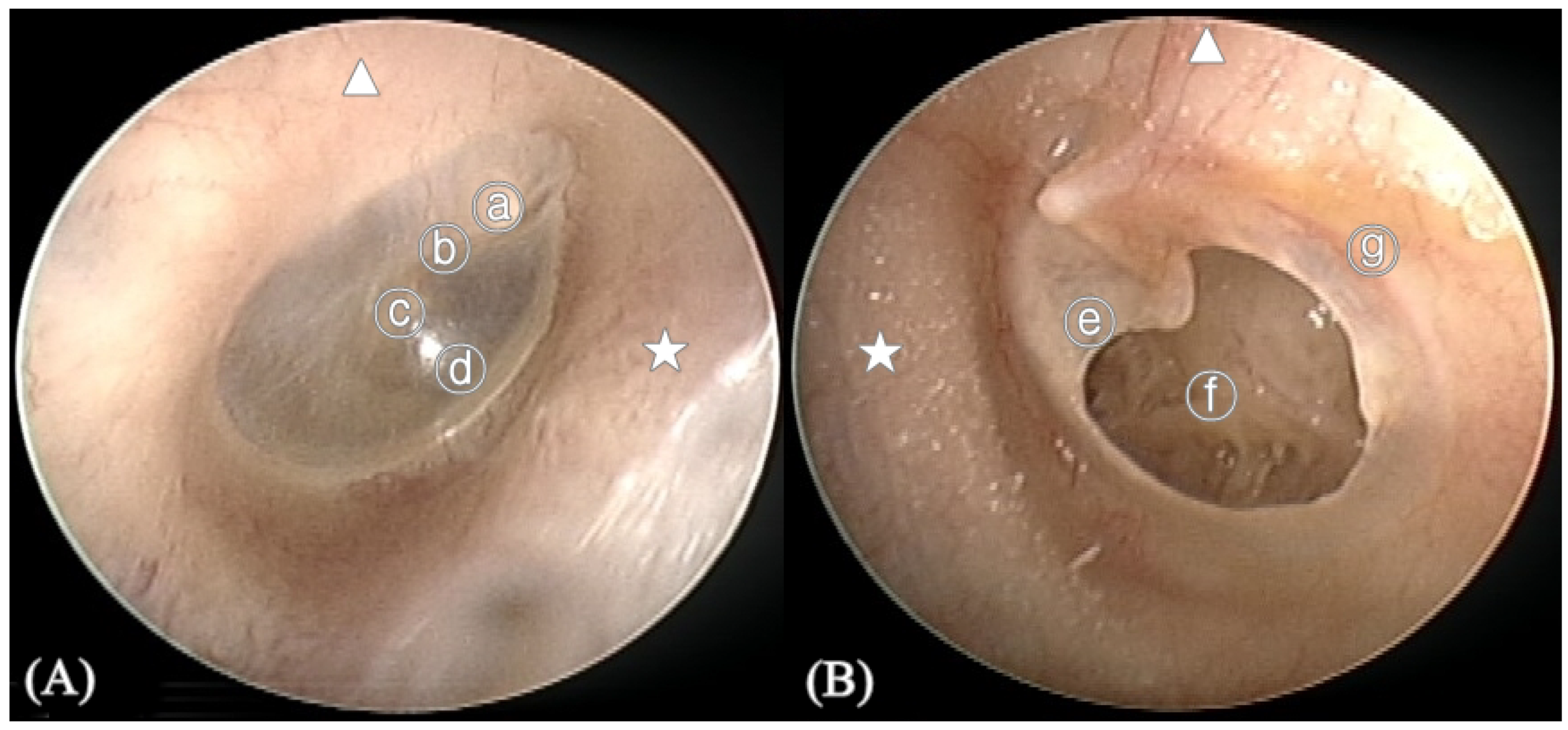
Figure 2.
Anatomy of the tympanic membrane (TM). (A) Right normal TM (B) Left TM with perforation. ⓐ Malleus short process, ⓑ Handle of malleus, ⓒ Umbo, ⓓ Cone of light, ⓔ Perforation margin, ⓕ Middle ear, ⓖ Annulus of TM, ★ Anterior of external auditory canal, ▲ Superior of external auditory canal.

Figure 3.
Class activation maps (CAM). CAM is a colored representation of data where different values are represented as different colors with values ranging from blue to red (blue, cyan, green, yellow, red). The red regions in the overlay image represent the most specific discriminative parts of the image by the deep neural network. The blue regions represent the non-specific part. (A) Right side tympanic membrane (TM) image with perforation. (B) Left side TM image without perforation.


Table 1.
Test phase accuracy.
| Label | Side | Perforation |
|---|---|---|
| Left normal (663) | 96.5% | 89.1% |
| Right normal (773) | 99.2% | 91.7% |
| Left perforated TM (181) | 95.6% | 91.1% |
| Right perforated TM (201) | 99.5% | 94.5% |
| Overall (1818) | 97.9% | 91.0% |
TM: tympanic membrane.
Table 2.
Diagnostic performance of the CNN.
| AUROC | Accuracy | Sensitivity | Specificity | PPV | NPV | |
|---|---|---|---|---|---|---|
| Side | 0.98 | 97.9% | 99.3% | 96.3% | 96.9% | 99.1% |
| Perforation | 0.92 | 91.0% | 90.5% | 92.9% | 98.0% | 72.3% |
AUROC = area under the receiver operating characteristic curve; PPV = positive predictive value; NPV = negative predictive value.
Table 3.
Activation rate of subsite in class activation map.
| Left Normal TM | Left TM with Perforation | Right Normal TM | Right TM with Perforation | ||||||||||
|---|---|---|---|---|---|---|---|---|---|---|---|---|---|
| Overall | Side | TM Finding | Overall | Side | TM Finding | Overall | Side | TM Finding | Overall | Side | TM Finding | ||
| Activation rate | 8.7% | 8.7% | 8.6% | 94.8% | 90.6% | 99.4% | 52.5% | 94.3% | 10.6% | 60.3% | 21.6% | 98.5% | |
| External auditory canal | AS | 19.1% | 1.5% | 1.8% | 42.3% | 30.4% | 50.3% | 46.5% | 47.3% | 1.4% | 41.9% | 8.0% | 42.3% |
| AI | 52.2% | 5.6% | 3.5% | 51.6% | 58.0% | 40.3% | 86.8% | 87.8% | 3.2% | 59.8% | 15.6% | 56.2% | |
| PS | 44.3% | 6.8% | 0.9% | 74.3% | 75.1% | 66.3% | 87.4% | 90.8% | 0.9% | 53.5% | 8.0% | 56.2% | |
| PI | 36.5% | 4.4% | 2.0% | 63.3% | 64.6% | 55.8% | 56.8% | 57.6% | 2.1% | 48.5% | 6.5% | 51.7% | |
| Tympanic membrane | AS | 20.9% | 1.1% | 2.6% | 31.2% | 44.2% | 15.5% | 22.7% | 22.5% | 1.3% | 17.4% | 3.5% | 17.4% |
| AI | 16.5% | 1.2% | 1.7% | 17.5% | 22.1% | 11.6% | 23.6% | 21.5% | 3.2% | 13.3% | 2.5% | 13.4% | |
| PS | 33.0% | * 5.3% (17.56) | 0.5% | 42.6% | 56.9% | 240.3% | 74.2% | 77.1% | 0.8% | 36.1% | 7.5% | 35.8% | |
| PI | 24.3% | * 2.3% (37.87) | 2.0% | 29.4% | 43.6% | 12.7% | 34.5% | 34.3% | 1.9% | 16.2% | 3.5% | 15.9% | |
| Tympanic annulus | AS | 20.9% | 2.0% | 1.7% | 24.2% | 12.2% | 33.7% | 48.8% | 50.2% | 1.0% | 24.5% | 1.0% | 28.4% |
| AI | 25.2% | 3.2% | 1.2% | 30.3% | 20.4% | 37.0% | 59.4% | 59.9% | 2.5% | 32.0% | 1.5% | 36.8% | |
| PS | 44.3% | 6.9% | 0.8% | 25.7% | 32.0% | 16.6% | 85.9% | 89.0% | 1.2% | 13.3% | 3.5% | 12.4% | |
| PI | 21.7% | 2.9% | 0.9% | 14.9% | 7.7% | 20.4% | 46.9% | 48.3% | 0.9% | 28.6% | 0% | 34.3% | |
| Malleus | Short process | 45.2% | 7.2% | 0.6% | 49.3% | 61.9% | 31.5% | 89.9% | 93.1% | 1.2% | 43.2% | 10.1% | 41.8% |
| Handle | 27.8% | 4.1% | 0.8% | 19.8% | 16.0% | 22.1% | 72.9% | 75.0% | 1.4% | 16.2% | 1.5% | 17.9% | |
| Cone of light | 46.1% | 6.5% | 1.5% | 2.0% | 2.8% | 1.1% | 74.8% | 77.7% | 0.8% | 4.1% | 1.5% | 3.5% | |
| Umbo | 22.6% | 3.3% | 0.6% | 7.0% | 6.1% | 7.2% | 60.3% | 62.7% | 0.5% | 9.1% | 0.5% | 10.4% | |
| Perforation margin | 0% | 0% | 0% | 43.4% | 19.9% | * 63.0% (9.03) | 0% | 0% | 0% | 53.9% | 1.5% | 63.2% | |
| Middle ear | 0% | 0% | 0% | 61.8% | 39.2% | * 78.5% (3.55) | 0% | 0% | 0% | 75.9% | 10.1% | * 81.1% (37.88) | |
AS: Anterior-superior, AI: Anterior-inferior, PS: Posterior-superior, PI: Posterior- inferior. *: statistically significant (p < 0.0.5), ( ): Odd ratio.
© 2019 by the authors. Licensee MDPI, Basel, Switzerland. This article is an open access article distributed under the terms and conditions of the Creative Commons Attribution (CC BY) license (http://creativecommons.org/licenses/by/4.0/).
Share and Cite
MDPI and ACS Style
Lee, J.Y.; Choi, S.-H.; Chung, J.W. Automated Classification of the Tympanic Membrane Using a Convolutional Neural Network. Appl. Sci. 2019, 9, 1827. https://doi.org/10.3390/app9091827
AMA Style
Lee JY, Choi S-H, Chung JW. Automated Classification of the Tympanic Membrane Using a Convolutional Neural Network. Applied Sciences. 2019; 9(9):1827. https://doi.org/10.3390/app9091827
Chicago/Turabian StyleLee, Je Yeon, Seung-Ho Choi, and Jong Woo Chung. 2019. "Automated Classification of the Tympanic Membrane Using a Convolutional Neural Network" Applied Sciences 9, no. 9: 1827. https://doi.org/10.3390/app9091827
Note that from the first issue of 2016, this journal uses article numbers instead of page numbers. See further details here.