A Novel Binary Competitive Swarm Optimizer for Power System Unit Commitment

Abstract

The unit commitment (UC) problem is a critical task in power system operation process. The units realize reasonable start-up and shut-down scheduling and would bring considerable economic savings to the grid operators. However, unit commitment is a high-dimensional mixed-integer optimisation problem, which has long been intractable for current solvers. Competitive swarm optimizer is a recent proposed meta-heuristic algorithm specialized in solving the high-dimensional problem. In this paper, a novel binary competitive swarm optimizer (BCSO) is proposed for solving the UC problem associated with lambda iteration method. To verify the effectiveness of the proposed algorithm, comprehensive numerical studies on different sizes units ranging from 10 to 100 are proposed, and the algorithm is compared with other counterparts. Results clearly show that BCSO outperforms all the other counterparts and is therefore completely capable of solving the UC problem.

1. Introduction

Given the continuous increase of electricity demand and unbalanced demand distribution, proper adjustment of the unit status in order to realize rational use of the generation power resource is of significant importance to the power system operators [1]. The normal method to solve the UC problem is to minimize the economic cost and pollutant emissions by arranging to start-up or shut-down the units while meeting various practical constraints including power demand balance, generation limit, etc. [2]. Due to the remarkable complexity, constraints and binary switching effect of the system [3], UC is widely regarded as a nonlinear, multi-constraint, large-scale and mixed-integer problem.

Many optimization algorithms have attempted to solve the UC problem. Some traditional mathematical methods, such as the dynamic programming [4], integer programming [5], mixed-integer programming [6], branch and bound methods [7], evolutionary programming [8] and Lagrangian relaxation methods [9,10] have been employed. Apparent advantages and defects can be found with these algorithms. For example, the Lagrangian relaxation methods is suitable for solving the large-scale constrained problem; however, the algorithm may oscillate during the iteration and the convergence speed is slow. Dynamic programming method is suitable for solving the problems of multi-stage decision process optimization, whereas it is easy to cause dimensional disaster in high-dimensional applications.

With development of the meta-heuristic (MA) optimization algorithms, many scholars have applied the evolutionary based MA approaches to solve the UC problem. Generally speaking, MA approaches construct algorithmic logic based on common phenomena in nature and life, and maintain a single or a population of available solutions to search for the optimal solution for complex problems. Featured MA tools have been adopted in solving UC problem include genetic algorithms (GAs) [11,12], simulated annealing (SA) [13], particle swarm optimization (PSO) [14] and ACO [15], as well as teaching-learning based optimization (TLBO) [16], etc. Some popular PSO variants such as binary particle swarm optimization (BPSO) [17,18], symmetric binary particle swarm optimization [19], quantum-inspired particle swarm optimization (QPSO) [20], hybrid particle swarm optimization (HPSO) [21,22] etc., have also been used. Additionally, other variants of PSO algorithm have been applied in some engineering application, for example, the Bluetooth energy management and model updating [23,24].

Inspired by the PSO algorithm and to further increase the refinement ability, Cheng and Jin proposed the competitive swarm optimizer (CSO) [25] in 2015. The CSO adopts a novel learning mechanism without the use of $g_{best}$ and $P_{best}$. It demonstrates competitions between particle pairs, and the losers should update their velocity and position by learning from the winner. Although the principle of CSO is fairly simple, the performance of convergence speed and optimum result is considerably improved compared to its ancestor PSO, and this competitive mechanism has effectively solved the large-scale optimization problem with high dimension and complexity. CSO and its variants have been used to optimal installation of multiple distributed generation (DG) units [26], economic dispatch [27,28] and other large-scale power system problems [29].

In this paper, a novel BCSO algorithm is proposed for solving the UC problem. The major contributions of the paper are shown as below:

(1)

To solve the problem of binary switching in the engineering application, a novel binary competitive swarm optimization (BCSO) algorithm has been proposed based the framework of CSO algorithm.

(2)

The proposed BCSO algorithm was applied to solve the UC problem with different unit number, which provided a new method for solving large-scale optimization problems.

(3)

The feasibility and practicability of the proposed algorithm and the applicability for large-scale, mixed-integer problems was validated, through the comprehensive experimental analysis.

The rest of the paper is allocated as follows: The UC problem formulation is presented in Section 2. The BCSO algorithm is then proposed in Section 3, followed by the detailed demonstration of the process for BCSO solving UC problem presented in Section 4. The experimental results and numerical analysis are given in Section 5. Finally, Section 6 concludes the paper.

2. Problem Formulation

The UC problem is occupying an outstanding position in the electric power system operation area due to its complexity and importance. The efficient optimization of UC problem can effectively reduce economic cost given that even 1% decrease would save millions of dollars a year. Generally, the economic cost of units during a 24 h day horizon is modeled as the objective function for UC problem. Meanwhile, it also needs to satisfy several equality and inequality constraints, for example, power demand limit, spinning reserve limit, generation limit, etc. In this section, the formulation of objective function and constraints conditions will be addressed.

2.1. Objective Function

Traditionally, the UC problem considered the duration within one hour as a single value, and it does not consider the effect between each time period. In this paper, the economic cost is the sum of costs of units within 24 h as shown in Formula (1) below.

$$TP{C}_{T\mathrm{n}}=\min {\displaystyle \sum _{t=1}^T{\displaystyle \sum _{j=1}^n[F_j(P_{j,t})u_{j,t}+S{U}_{j,t}(1-u_{j,t-1})u_{j,t}]}}$$

(1)

In Formula (1), the total economic cost $TP{C}_{Tn}$ is composed of two parts, namely fuel cost and start-up cost respectively. The start-up cost is generated at the moment of the unit start. $F_j(P_{j,t})$ is the fuel cost function of the jth unit, and generation output is denoted as $P_{j,t}$ during the $t$ hour. $S{U}_{j,t}$ is the star-up cost of the jth unit during the t time, and $u_{j,t}$ is the status of jth unit at the $t$ hour described by 0 or 1.

2.1.1. Fuel Cost

The fuel cost can be described by a quadratic polynomial formulation, as Formula (2) shows:

$$F_{j,t}(P_{j,t})=a_j+b_j{P}_{j,t}+c_j{P}^2{}_{j,t}$$

(2)

where $a_j$, $b_j$ and $c_j$ are the fuel cost coefficients of the jth unit.

2.1.2. Start-Up Cost

Due to the running time limit and other restrictions, the unit start-up requires an extra cost of the fuel. The cost of start-up is therefore an indispensable part for the total economic cost. It is described by Formula (3):

$$S{U}_{j,t}=\left\{\begin{array}{l}S{U}_{H,j},ifMD{T}_j\le TOF{F}_{j,t}\le MD{T}_j+T_{cold,j}\\ S{U}_{C,j},ifTOF{F}_{j,t}>MD{T}_j+T_{cold,j}\end{array}\right\}$$

(3)

The start-up cost of a unit may be categorized as hot start and cold start. When a unit has been turned off for a short period of time, it is calculated as hot start. Otherwise, cold start cost may have to be taken into account. Therefore, the start-up cost is closely related to the previous running status and current status of the unit. In this section, $S{U}_{H,j}$ indicates the hot start-up cost of the jth unit, and the $S{U}_{C,j}$ denotes the cold start-up cost of the jth unit. $T_{cold,j}$ is the cold start hour of the jth unit. $MD{T}_j$ denotes the minimum down time of jth unit, and $MU{T}_j$ denotes the minimum up time of jth unit. $TOF{F}_{j,t}$ represents the continuous time of the jth unit with off status.

2.2. Constraints

Different numbers of on-line units require many factors to be considered during the different time period. System constraints covering the unit condition limitations, interaction of each unit between different time periods, etc. The precondition for achieving the optimal economic cost objective function should meet the different constraint limits. The common limits are the power balance constrains, generation limit constraint, spinning reserve constraint, etc. There are others limits, for example, the ramping rate constraints, valve-point effect and emission constraints. In this paper, only major constraints are considered for simplification.

2.2.1. Power Balance Constraint

In actual industrial power generation, the power demand keeps changing all the time. To meet the power balance constraint is an important and foremost task in the scheduling. The power balance constraint is an equality constraint, shown as the following Formula (4):

$${\displaystyle \sum _{j=1}^n{P}_{j,t}{u}_{j,t}=P_{D,t}}$$

(4)

where $P_{D,t}$ is the power demand at time $t$. In this paper, the power loss in the transmission process is ignored. It is denoted that the generation output power of the unit jth at time $t$ should be balanced with the load demand of the system, which means the supply should be equaled to the demand. Otherwise, the frequency and voltage may vibrate and lead to black out or other security problem [30,31].

2.2.2. Generation Limit Constraint

The generation limit constraint of the unit is regarded as one of a physical constraint. This inequality constraint limits the unit output to a certain range due to the generation capacity of the corresponding unit. It is shown in the following formula:

$$u_{j,t}{P}_{j,\min }\le P_{j,t}\le u_{j,t}{P}_{j,\max }$$

(5)

where $P_{j,\min }$ represents the minimum power generation, and $P_{j,\max }$ denotes the maximum power capacity.

2.2.3. Minimum Up/Down-Time Limit Constraint

As shown in the following Formula (6), the status shifting of different units are restrained by this constraint, which is related to the $MU{T}_j$ and $MD{T}_j$. In the unit system, the state only has two cases. If the state of unit is 1, it means the unit is on-line, and vice versa.

$$u_{j,t}=\left\{\begin{array}{l}1,if1\le TO{N}_{j,t-1}<MU{T}_j\\ 0,if1\le TOF{F}_{j,t-1}<MD{T}_j\\ 0or1,otherwise\end{array}\right\}$$

(6)

In the Formula (6), $TO{N}_{j,t-1}$ is denoted as the continuous opening time, and $TOF{F}_{j,t-1}$ is the close time. If the running time of the unit jth is less than $TO{N}_{j,t-1}$, the unit should be turned on. Otherwise, it should be turned off. If the close time of the unit jth is less than $TO{N}_{j,t-1}$, the unit should be off-line. The running time or close time is also related to the start-up economic cost.

2.2.4. Spinning Reserve Limit Constraint

Because of that the load demand of the system is not the actual value, the existence of spinning reserves is important to deal with unexpected extra load and to effectively achieve power balance demand. The balance is an equal constraint shown in the following Formula (7):

$${\displaystyle \sum _{j=1}^n{P}_{j,\max }{u}_{j,t}=P_{D,t}+S{R}_t}$$

(7)

where the $S{R}_t$ is the spinning reserves during the time $t$. Under normal conditions, the spinning reserves accounts for a certain proportion of load demand, denoted as $S{R}_t=m*P_{D,t}$. The value of $m$ is set as 0.1 in this paper.

The parameter settings of $P_{D,t}$, $MU{T}_j$, $MD{T}_j$ and many others are illustrated in the

Table 1. Parameter setting for Binary Competitive Swarm Optimizer (BCSO).

	Unit 1	Unit 2	Unit 3	Unit 4	Unit 5	Unit 6	Unit 7	Unit 8	Unit 9	Unit 10
Pmax (MW)	455	455	130	130	162	80	85	55	55	55
Pmin (MW)	150	150	20	20	25	20	25	10	10	10
a ($/MW h)	1000	970	700	680	450	370	480	660	665	670
b ($/MW h)	16.19	17.26	16.6	16.5	19.7	22.26	27.74	25.92	27.27	27.79
c ($/MW h)	0.00048	0.00031	0.002	0.00211	0.00398	0.00712	0.000793	0.00413	0.002221	0.00173
MU (h)	8	8	5	5	6	3	3	1	1	1
MD (h)	8	8	5	5	6	3	3	1	1	1
Hot Start Cost (\$)	4500	5000	550	560	900	170	260	30	30	30
Cold Start Cost (\$)	9000	10,000	1100	1120	1800	340	520	60	60	60
Initial Status (h)	1	1	0	0	0	0	0	0	0	0

. When searching for the optimal solution of the objective function, all constraints should be satisfied. That will be described in detail in Section 4.

3. Proposed Binary Competitive Swarm Optimizer

The algorithm is inspired by particle swarm optimization whereas adopts a brand-new particle evolutionary scheme. The particles of PSO update their speed and locations mainly based on the $P_{best}$ and $g_{best}$, where $P_{best}$ is the best position of each particle among the evolutionary process and $g_{best}$ is the global best position along the whole iterations. However, the CSO maintains a completely different evolutionary strategy compared with PSO. Its update method is mainly realized by the mutual competition learning mechanism between particles, solving the large-scale function with good optimization performance. Additionally, this method has many applications for complex economic dispatch and unit commitment optimization problems. Inspired by the original CSO, a novel binary CSO method is proposed in this paper for solving the UC problem.

3.1. Competitive Swarm Optimization

In CSO algorithm, a novel pairwise competition mechanism between the particles is proposed. The $P_{best}$ and $g_{best}$ are removed, and the particles update their velocity and position by learning from the winner, which has the better fitness compared with the opponent particle. In the algorithm, suppose a population of particle $P_t$ containing $m$ particles. Each particle has two characteristics including position and velocity. The positions of these particles are denoted by $X_i(t)=(x_{(i,1)}(t),x_{(i,2)}(t),\dots x_{(i,n)}(t))$, and $n$ is the dimension of the particles. The velocity is denoted by $v_i(t)=(v_{(i,1)}(t),v_{(i,2)}(t),\dots v_{(i,n)}(t))$. In the beginning, the position and velocity of the particles are initialized randomly and constantly updated with the iteration. In each generation, the swarm $P_t$ is randomly divided into $m/2$ couples and the particles of each couple are a competing objects pair. In the integrated process, there will be $m/2$ times competitions, where the fitness of these particle will be compared. If the fitness value of one particle is better, it will be defined as the winner; Otherwise, the other particle is defined as the loser. The loser should update its velocity and position through learning from the winner.

Suppose in the kth competition, the position of loser particle is described by $X_{l,k}(t)$, and its velocity is denoted by $V_{l,k}(t)$, where $k=1,2,\dots ,m/2$. After the competition, the velocity of loser will be updated according to the evolutionary logic, which is shown in the following Equation (8):

$$V_{l,k}(t+1)=R_1(k,t)V_{l,k}(t)+R_2(k,t)(X_{w,k}(t)-X_{l,k}(t))+\varphi R_3(k,t)(X^{\text{'}}{}_k(t)-X_{l,k}(t))$$

(8)

where $X_{w,k}(t)$ is denoted as the position of the winner particle. $R_1(k,t),R_2(k,t)$ and $R_3(k,t)$ are the randomly produced vectors in the generation t between 0 and 1. $V_{l,k}(t+1)$ represents the velocity of loser after the kth competition. $X^{\text{'}}{}_k(t)$ is the mean position value of the swam particle $P_t$. $\varphi$ is the only algorithm specific parameter in the algorithm and it controls the influence of $X^{\text{'}}{}_k(t)$ in the optimization process. Therefore, the parameter setting is more important.

The position of the loser will be updated along with the velocity update as shown in the following equation:

$$X_{l,k}(t+1)=X_{l,k}(t)+V_{l,k}(t+1)$$

(9)

where $X_{l,k}(t+1)$ denotes the position of the winner particle after the $k_{th}$ competition. It is related to the velocity of loser after the competition. After the competition, the winner particle will be directly put into the swarm $P_{t+1}$ for the next generation, while the loser will be thrown into the swarm $P_{t+1}$ after update of velocity and position. Therefore, each particle has only one chance to take part in the competition. The only one parameter scheme of this algorithm reduces the parameter tuning work of the CSO. Meanwhile, the novel scheme significantly improves the algorithm performance. In essence, the CSO is more suitable for solving large-scale optimization problems.

3.2. Proposed Binary CSO

The original CSO algorithm has been applied to many practical real-valued optimization problems. However, there are also numerous large-scale discrete problems remaining to be solved such as UC. In this section, a novel binary CSO in proposed. Inspired by evolutionary logic and discrete PSO algorithm, the binary decision variables are determined by a transfer function from the updated velocity. To improve the efficiency of the evolution, a V-shape transfer function (10) is adopted. The detailed transfer function is defined as follows:

$$S(V_{i,j})=2\cdot |\frac{1}{(1+e^{(-V_{i,j})})}-0.5|$$

(10)

where the result of this function $S(V_{i,j})$ is a proportional value, it decides the value of $X_i(t)$ according to (11). The velocity $V_{i,j}$ will be limited to a certain range after the initialization. In this paper, the velocity is limited to [−4, 4].

$$x_{i,j}=\left\{\begin{array}{l}1,ifrand<S(V_{i,j})\\ 0,otherwise\end{array}\right\}$$

(11)

In Equation (11) $rand$ is a number generated random, the range of it is [0, 1]. If the $S(V_{i,j})$ greater than $rand$, the particle is 0. The novel BCSO method will be adopted in determining the binary status of UC problem and the detailed procedure will be illustrated in the next section.

4. BCSO Application to UC

The process of handling the constraints conditions must be carried out in the unit commitment. In this section, the constraint handling process and the proposed BCSO for UC problem will be demonstrated. The constraints handling includes the power balance limit, generation limit and minimum up- and down-time limit, etc.

4.1. Constraints Processing

The particle will undergo constraint checks after the initialization. According to Formula (6), the state of particle is judged whether it has met the minimum up/down-time limit constraint. Once violation has occurred, a corresponding technique [32] will be conducted to fix the solution and make it meet the limit. Next, the particles are checked for the spinning reserve limit constraint according to (7). A heuristic-based handling approach [30] is adopted to handle this. Specifically, if the accumulated generation output power is larger than the sum of load and spinning reserve, some units should be turned off. Otherwise, it should take measures to ensure more units are on-line. The process of power demand balance constraint is embedded in the lambda iteration method where a tiny lambda value is tuned. The handling of the generation limit constraint (5) is also embedded in the lambda iteration method acting as the upper and lower boundaries.

4.2. Applied BCSO to UC

In addition to the handling of the constraints, the proposed BCSO is applied in the UC problem to find the fitness of the objective function, determining economic optimum through the evolutionary search for the unit start-up and shut-down. The steps of the algorithm are shown as follows:

4.2.1. Initialization

• Set the parameters of the power system such as the load demand, the fuel cost coefficients of the unit, generation capacity and minimum up/down time, etc.;
• Initialize for the parameters of BCSO such as $\varphi$ and maximum iteration time;
• Initialize and boundary check of the particles and their velocity, generate the value of the particle according to Equations (10) and (11), then check the constraints;

4.2.2. BCSO Process

• Divide particles into $m/2$ couples, compute objective function of each particle in couple, determine the loser and winner;
• Update the velocity of the loser according Equation (8) and check the boundary;
• Update the value of the loser according to Equations (10) and (11), and check the constraints to generated the new swarm;
• If the iteration is less than the maximum value of the iteration, go back to the first step of BCSO process. Otherwise, end the process and output the result.

In this section, the proposed BCSO method is adopted for solving the UC problem. The experimental results are expressed in the following section.

5. Experimental Results and Analysis

In the numerical study, the parameters of BCSO algorithm and data setting will be briefly introduced, and the method BCSO is applied for different unit numbers, such as 10, 20 and 40 units. All the case studies are simulated on an Intel(R) Core(TM) i7-3537U CPU @ 2.50 GHz PC and the Matlab (R) 2017a software platform. The experimental result will be compared with different algorithms to prove that the competitive performance of proposed BCSO algorithm for solving the UC problem.

5.1. Parameter of BCSO and Data Setting

In all the case studies, the population size is 150, and the maximum iteration is 200. The velocities of particles are set from −4 to 4. The dimension increases along with the unit numbers increase, where the range of dimension rise from 240 to 2400 for the binary decision viable, associated with the same scale of real-valued variables for power output of the corresponding units. With the dimension increases, the only algorithm parameter $\varphi$ in the BCSO increases from 0.0 to 0.3. Additionally, the data settings are listed in Table 1.

5.2. The Experimental Results of BCSO

The BCSO algorithm is applied to the different trials to test the performance. To eliminate the randomness, algorithms run 30 independent trials from different initial populations in each trial and get the mean, best and worst values. The

Table 2. Comparison between BCSO and other algorithms.

Methods	Trials	Population	Iteration	Best ($)	Mean ($)	Worst ($)	STDV	Time (s)
IBPSO	10	20	2000	563,777	564,155	565,312	143	27
IPSO	50	40	1000	563,954	564,162	564,579	-	-
HPSO	100	20	1000	563,942.3	564,772.3	565,785.3	-	-
QBPSO	50	-	1000	563,977	563,977	563,977	0.00	18
GA	20	50	500	565,852	-	570,032	-	221
SA	-	-	50	565,828	565,988	566,260	-	3.35
brGA	30	-	1000	563,938	564,253	564,088	18	-
DBDE	20	40	1000	563,977	564,028	564,241	103	3.6
BDE	50	20	1000	563,977	563,977	563,977	0.00	-
BGSO	50	50	-	563,938	563,952	564,226	-	3
BPSO	30	150	200	563,955.99	564,000.40	564,053.73	21.63	25.45
BLPSO	30	150	200	563,977.01	563,982.09	563,987.16	-	22.09
NBPSO	30	150	200	563,937.68	563,962.59	563,977.01	-	21.91
BCSO	30	150	200	563,937.68	563,937.68	563,937.68	0.00	11.58

shown the comparison result between BCSO and improved binary particle swarm optimization (IBPSO), improved particle swarm optimization (IPSO), hybrid particle swarm optimization (HPSO), quantum-inspired particle swarm optimization (QPSO), genetic algorithm (GA), simulated annealing (SA), binary- real-code GA (brGA), discrete binary differential evolution (DBDE), binary differential evolution (BDE), binary glowworm swarm optimization (BGSO), binary particle swarm optimization (BPSO), best parallel particle swarm optimization (BLPSO), and new binary particle swarm optimization (NBPSO) algorithm with the unit is 10, from it can see that the optimum result of NBPSO and BCSO are 563,937.68 $/day, but BCSO has an advantage in the worst cost among all the algorithms, and the stability of BCSO is proven. The experimental results of different unit numbers used BCSO are shown in

Table 3. Statistic experimental result of BCSO for different Unit numbers.

Units	Best ($)	Mean ($)	Worst ($)	Time (s)
10	563,937.68	563,937.68	563,937.68	11.58
20	1,124,389.73	1,124,477.52	1,124,524.29	20.15
40	2,246,837.71	2,247,351.83	2,247,675.59	35.02
60	3,367,348.99	3,367,466.61	3,367,535.33	49.45
80	4,491,212.46	4,491,574.93	4,491,717.60	66.91
100	5,610,281.71	5,610,624.74	5,610,986.92	85.01

. It can be seen from the table, when the unit is 10, the optimum solution of the BCSO is 563,937.68 $/day, and the worst fuel cost is 563,937.68 $/day. From the mean, best and worst values, the fluctuation of the optimum solutions can be compared. It can also be seen from the result that all the corresponding values obtained by BCSO are comparatively small. The convergence curve of BCSO for the 10-unit case is shown in Figure 1, demonstrating that the convergence speed of BCSO is fast and can obtain the optimal solution within around 30 iterations.

There are many algorithms that have been used to solve the UC problem, for example, BPSO, BLPSO and NBPSO [33]. The first picture in Figure 1 shows the convergence curve of the four algorithms in the 10-unit problem, illustrating that the convergence speed of BCSO significantly outperforms the other methods. The

Table 4. Comparisons using different methods for different Unit numbers.

Units	Methods	Best ($)	Mean ($)	Worst ($)	Time (s)
10	BCSO	563,937.68	563,937.68	563,937.68	12.51
	BPSO	563,955.99	564,000.40	564,053.73	21.56
	BLPSO	563,777.01	563,982.09	563,987.16	21.01
	NBPSO	563,937.68	563,962.59	563,977.01	21.05
20	BCSO	1,124,389.73	1,124,477.52	1,124,524.29	20.15
	BPSO	1,127,588.66	1,129,897.11	1,131,708.18	32.32
	BLPSO	1,126,027.27	1,126,195.45	1,126,748.06	31.32
	NBPSO	1,128,147.58	1,128,157.00	1,128,218.22	33.28
40	BCSO	2,246,837.71	2,247,351.83	2,247,675.59	35.02
	BPSO	2,260,669.13	2,267,206.95	2,273,667.73	51.77
	BLPSO	2,254,213.53	2,254,289.66	2,254,967.89	51.72
	NBPSO	2,261,696.75	2,261,696.75	2,261,696.75	53.17
60	BCSO	3,367,348.99	3,367,466.61	3,367,535.33	49.45
	BPSO	387,761.20	3,395,743.16	3,404,382.46	69.09
	BLPSO	3,384,093.39	3,393,103.18	3,395,468.84	66.68
	NBPSO	3,395,480.43	3,395,480.43	3,395,480.43	69.39
80	BCSO	4,491,212.46	4,491,574.93	4,491,717.60	66.91
	BPSO	4,524,683.47	4,538,115.06	4,547,525.84	103.94
	BLPSO	4,513,521.52	4,520,667.44	4,522,452.92	98.97
	NBPSO	4,530,843.70	4,530,843.70	4,530,843.70	101.33
100	BCSO	5,610,281.71	5,610,624.74	5,610,986.92	85.01
	BPSO	566,545.61	5,482,671.50	5,692,414.71	112.45
	BLPSO	5,655,610.14	5,655,610.14	5,655,610.14	113.54
	NBPSO	5,648,702.49	5,648,702.49	5,648,702.49	121.56

shows the experimental result of BCSO compared with the other binary PSO variants. Comparing the data in Table 4, we can find that the optimum solution of the BCSO is the best, achieving 56,397.68 $/day. As for the 20, 40 or 60-unit tests, the BCSO method also gets the best results among the four contestants. It can be concluded that the BCSO applied to the UC problem can bring significant economic benefits compared with other counterparts.

The simulation result of BCSO and other algorithms is showed in Figure 1. This graph shows different convergence curves for the iteration process on different unit numbers. It can be observed that no matter what the number of units are, the green curve (representing the BCSO algorithm) always converged around the 20th iteration. When the unit number is 20, 40 and 60, the convergence speed of BLPSO algorithm was the same as that of BCSO, but the convergence speed of BLPSO is not stable, and it becomes slower with the dimension increase. The curve of BPSO and NBPSO algorithm converged slowly, and the optimum solution is worse than the BCSO algorithm. Therefore, it can be concluded that the convergence speed of BCSO algorithm is also of large advantage compared with others.

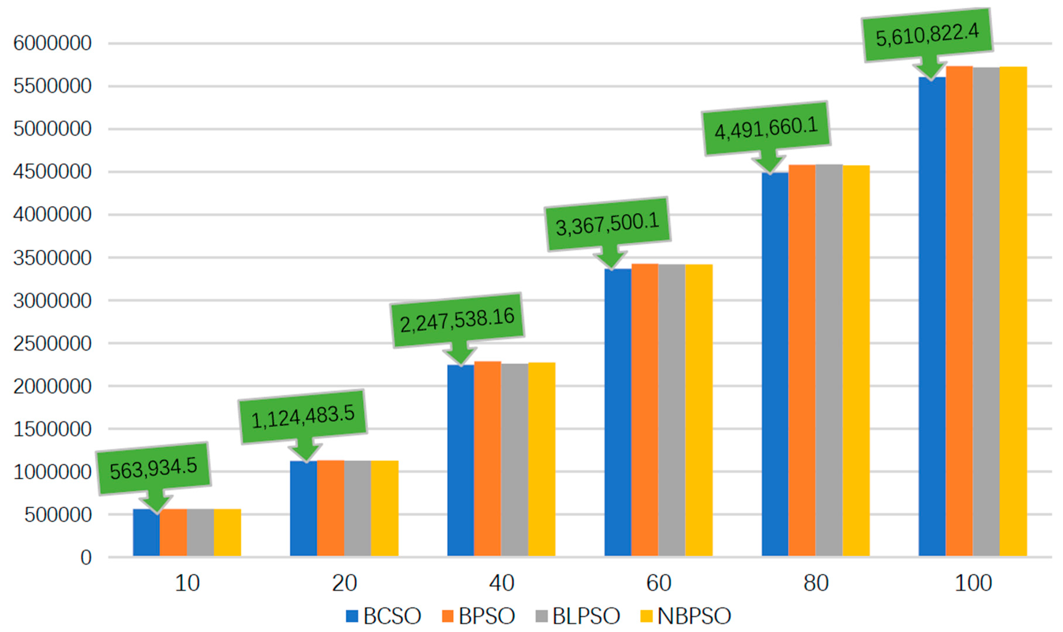
Figure 2 shows the mean values of the four contestant methods for solving different unit numbers. In Figure 2, the blue column of BCSO is the shortest, forming the point of economic cost, and the experimental results of the BCSO are the best. Combining the Table 4 and Figure 2, it can be proved that the BCSO algorithm is a competitive tool in solving UC problem. From Figure 2, it can be observed that the height difference gradually increases with the unit number increase, which means that the difference of optimum solution between the BCSO with other algorithms is increasing with the dimension scales increase. Thanks to the evolutionary advantage of BCSO, the proposed method is even more competitive in solving the large scales cases.

The run time curve of four heuristic algorithms with different unit numbers is shown in Figure 3. From Figure 3, it can be seen that the curve of BCSO (blue curve) is at the bottom, and it reflects that the run time of BCSO is the least. Comparing the interval between different curves, we find that the curves of BPSO, BLPSO and NBPSO have smaller intervals, for example, when the unit is 10 and 20, the three curves almost coincide, but the interval between BCSO and another algorithm is larger and the interval increases with the unit-scales increase. For example, when the unit is 10, the run time difference between BCSO and NBPSO is 8.54 s; when the unit increased to 100, the difference is increased to 35.55 s. It can be concluded that the calculating time of BCSO algorithm is not affected by high-dimensional issues. Therefore, the convergence speed and applicability of the proposed BCSO algorithm are proved again.

From the experimental results shown above, it can be concluded that the BCSO is able to improve the optimization accuracy and improve the economic effect. The BCSO algorithm converges quickly and obtains competitive results. This may due to the fact that the character of the UC problem is a high dimension and complicated problem, and the BCSO algorithm provides chances for further exploitation in each dimension, and is therefore more suitable for solving this kind of problem.

6. Conclusions

Unit commitment is an intractable problem in power systems which requires effective new approaches. In this paper, a novel BCSO method is proposed in solving the mixed-integer large-scale UC problem, minimizing the economic cost considering power demand balance limit, generation capacity limit and spinning reserve and other constrains. The proposed BCSO is investigated on a number of different unit systems, and compared with experimental results from state-of-the-art evolutionary algorithms. Numerical results show that the BCSO can get better results compared to the other algorithms, and it also converges comparatively faster. In a result, the proposed BCSO method provides a very competitive tool to solve the UC problem. Future work may be addressed on applying BCSO with the combination of ordinary CSO method for solving the more complicated UC and economic load dispatch problems with the integration of stochastic renewable energy generations and plug-in electric vehicles.

References

- Wood, A.J.; Wollenberg, B.F.; Sheblé, G.B. Power Generation, Operation, and Control; John Wiley & Sons: New York, NY, USA, 2013. [Google Scholar]
- Padhy, N.P. Unit commitment-a bibliographical survey. IEEE Trans. Power Syst. 2004, 19, 1196–1205. [Google Scholar] [CrossRef]
- Zheng, Q.P.; Wang, J.; Liu, A.L. Stochastic optimization for unit commitment—A review. IEEE Trans. Power Syst. 2015, 30, 1913–1924. [Google Scholar] [CrossRef]
- Snyder, W.L.; Powell, H.D.; Rayburn, J.C. Dynamic programming approach to unit commitment. IEEE Trans. Power Syst. 1987, 2, 339–348. [Google Scholar] [CrossRef]
- Kim, K.; Zavala, V.M. Large-Scale Stochastic Mixed-Integer Programming Algorithms for Power Generation Scheduling. In Altern. Energy Sources Technologies; Springer: Cham, Switzerland, 2016; pp. 493–512. [Google Scholar]
- Delarue, E.; D’Haeseleer, W. Adaptive mixed-integer programming unit commitment strategy for determining the value of forecasting. Appl. Energy 2008, 85, 171–181. [Google Scholar] [CrossRef]
- Cohen, A.I.; Yoshimura, M. A branch-and-bound algorithm for unit commitment. IEEE Trans. Power Appar. Syst. 1983, PAS-102, 444–451. [Google Scholar] [CrossRef]
- Juste, K.A.; Kita, H.; Tanaka, E.; Hasegawa, J. An evolutionary programming solution to the unit commitment problem. IEEE Trans. Power Syst. 1999, 14, 1452–1459. [Google Scholar] [CrossRef]
- Zhuang, F.; Galiana, F.D. Towards a more rigorous and practical unit commitment by Lagrangian relaxation. IEEE Trans. Power Syst. 1988, 3, 763–773. [Google Scholar] [CrossRef]
- Jiang, Q.; Zhou, B.; Zhang, M. Parallel augment Lagrangian relaxation method for transient stability constrained unit commitment. IEEE Trans. Power Syst. 2013, 28, 1140–1148. [Google Scholar] [CrossRef]
- Kazarlis, S.A.; Bakirtzis, A.G.; Petridis, V. A genetic algorithm solution to the unit commitment problem. IEEE Trans. Power Syst. 1996, 11, 83–92. [Google Scholar] [CrossRef]
- Yang, H.T.; Yang, P.C.; Huang, C.L. A parallel genetic algorithm approach to solving the unit commitment problem: Implementation on the transputer networks. IEEE Trans. Power Syst. 1997, 12, 661–668. [Google Scholar] [CrossRef]
- Simopoulos, D.N.; Kavatza, S.D.; Vournas, C.D. Unit commitment by an enhanced simulated annealing algorithm. IEEE Trans. Power Syst. 2006, 21, 68–76. [Google Scholar] [CrossRef]
- Abido, M.A. Optimal design of power-system stabilizers using particle swarm optimization. IEEE Trans. Energy Convers. 2002, 17, 406–413. [Google Scholar] [CrossRef]
- Simon, S.P.; Padhy, N.P.; Anand, R.S. An ant colony system approach for unit commitment problem. Int. J. Electr. Power Energy Syst. 2006, 28, 315–323. [Google Scholar] [CrossRef]
- Roy, P.K.; Sarkar, R. Solution of unit commitment problem using quasi-oppositional teaching learning based algorithm. Int. J. Electr. Power Energy Syst. 2014, 60, 96–106. [Google Scholar] [CrossRef]
- Gaing, Z.L. Discrete particle swarm optimization algorithm for unit commitment. In Proceedings of the 2003 IEEE Power Engineering Society General Meeting, Toronto, ON, Canada, 13–17 July 2003; Volume 1, pp. 418–424. [Google Scholar]
- Yang, Z.; Li, K.; Niu, Q.; Xue, Y. A comprehensive study of economic unit commitment of power systems integrating various renewable generations and plug-in electric vehicles. Energy Convers. Manag. 2017, 132, 460–481. [Google Scholar] [CrossRef]
- Yang, Z.; Li, K.; Guo, Y.; Feng, S.; Niu, Q.; Xue, Y.; Foley, A. A binary symmetric based hybrid meta-heuristic method for solving mixed integer unit commitment problem integrating with significant plug-in electric vehicles. Energy 2019, 170, 889–905. [Google Scholar] [CrossRef]
- Lau, T.W.; Chung, C.Y.; Wong, K.P.; Chung, T.S.; Ho, S.L. Quantum-inspired evolutionary algorithm approach for unit commitment. IEEE Trans. Power Syst. 2009, 24, 1503–1512. [Google Scholar] [CrossRef]
- Ting, T.O.; Rao, M.V.C.; Loo, C.K. A Novel Approach for Unit Commitment Problem via an Effective Hybrid Particle Swarm Optimization. IEEE Trans. Power Syst. 2006, 21, 411–418. [Google Scholar] [CrossRef]
- Kennedy, J.; Eberhart, R.C. A discrete binary version of the particle swarm algorithm. In Proceedings of the 1997 IEEE International Conference on Systems, Man, and Cybernetics Computational Cybernetics and Simulation, Orlando, FL, USA, 12–15 October 1997; Volume 5, pp. 4104–4108. [Google Scholar]
- Pau, G.; Collotta, M.; Maniscalco, V. Bluetooth 5 energy management through a fuzzy-pso solution for mobile devices of internet of things. Energies 2017, 10, 992. [Google Scholar]
- Tran-Ngoc, H.; Khatir, S.; De Roeck, G.; Bui-Tien, T.; Nguyen-Ngoc, L.; Abdel Wahab, M. Model Updating for Nam O Bridge Using Particle Swarm Optimization Algorithm and Genetic Algorithm. Sensors 2018, 18, 4131. [Google Scholar] [CrossRef]
- Cheng, R.; Jin, Y. A competitive swarm optimizer for large scale optimization. IEEE Trans. Cybern. 2015, 45, 191–204. [Google Scholar] [CrossRef]
- Kumarappan, N.; Arulraj, R. Optimal installation of multiple DG units using competitive swarm optimizer (CSO) algorithm. In Proceedings of the IEEE Congress on Evolutionary Computation (CEC), Vancouver, BC, Canada, 24–29 July 2016; pp. 3955–3960. [Google Scholar]
- Xiong, G.; Shi, D. Orthogonal learning competitive swarm optimizer for economic dispatch problems. Appl. Soft Comput. 2018, 66, 134–148. [Google Scholar] [CrossRef]
- Guo, Y.; Xiong, G. Large scale power system economic dispatch based on an improved competitive swarm optimizer. Power Syst. Prot. Control 2017, 45, 97–103. [Google Scholar]
- Zhang, W.X.; Chen, W.N.; Zhang, J. A dynamic competitive swarm optimizer based-on entropy for large scale optimization. In Proceedings of the 2016 Eighth International Conference on Advanced Computational Intelligence (ICACI), Chiang Mai, Thailand, 14–16 February 2016; pp. 365–371. [Google Scholar]
- Leccese, F. Rome, a first example of Perceived Power Quality of electrical energy: The telecommunication point of view. In Proceedings of the INTELEC 7—29th International Telecommunications Energy Conference, Rome, Italy, 30 September–4 October 2007; pp. 369–372. [Google Scholar]
- Dugan, R.C.; Mc Granaghan, M.F.; Santoso, S.; Beaty, H.W. Electric Power Systems Quality; McGraw-Hill: New York, NY, USA, 2004. [Google Scholar]
- Jeong, Y.W.; Park, J.B.; Jang, S.H.; Lee, K.Y. A new quantum-inspired binary PSO: Application to unit commitment problems for power systems. IEEE Trans. Power Syst. 2010, 25, 1486–1495. [Google Scholar] [CrossRef]
- He, Y.; Wang, Y.; Liu, J. A new binary particle swarm optimization for solving discrete problems. Comput. Appl. Softw. 2007, 24, 157–159. [Google Scholar]
Figure 1.
Optimal convergences using different algorithms for different unit numbers.
Figure 2.
The mean comparison of different methods for different unit scales. BCSO: Binary competitive swarm optimizer; BPSO: Binary particle swarm optimization; BLPSO: Best parallel particle swarm optimization; NBPSO: New binary particle swarm optimization.
Figure 3.
The time-curve comparison of different methods for different unit scales.