The Causal Connection between CO2 Emissions and Agricultural Productivity in Pakistan: Empirical Evidence from an Autoregressive Distributed Lag Bounds Testing Approach


Abstract
:1. Introduction
2. Related Literature
3. Materials and Methods
3.1. Sources of Data
3.2. Econometric Model Specification
3.3. Specification of ARDL Model
4. Results and Discussion
4.1. Summary Statistics and Correlation Matrix
4.2. Unit Root Test Results
4.3. Cointegration Test
4.4. Long-Run and Short-Run Evidence
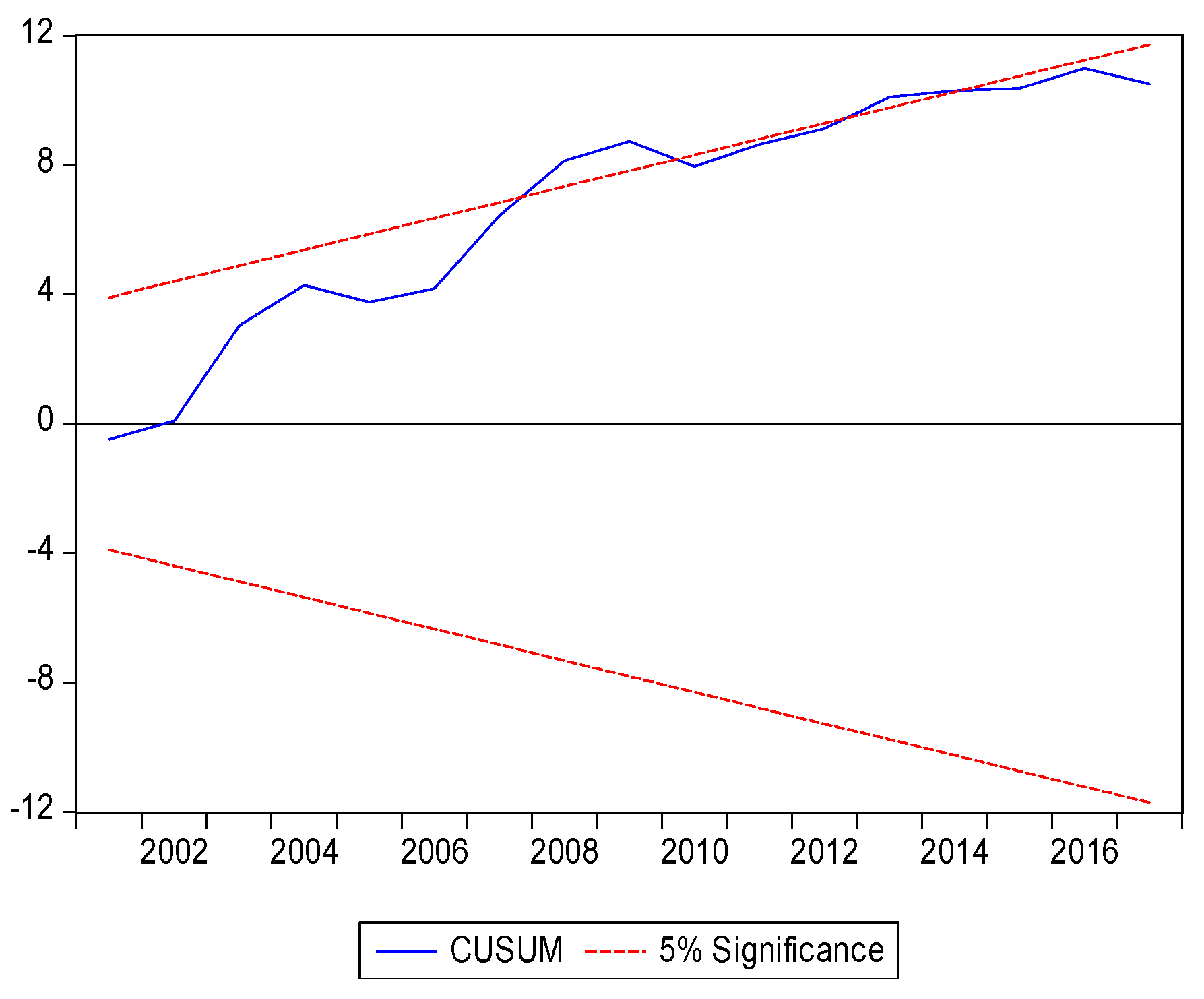
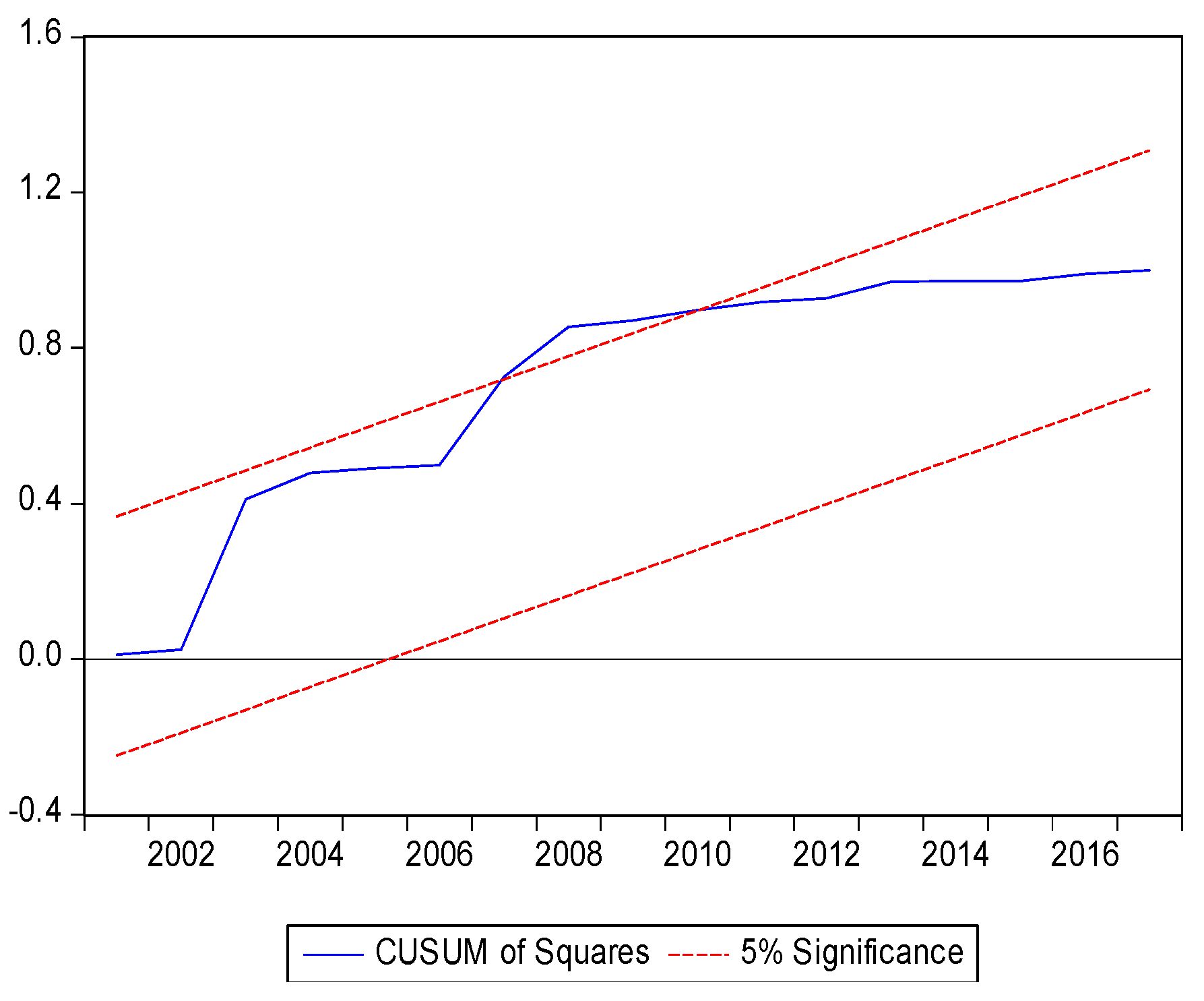
4.5. Structural Stability Test
5. Conclusion and Recommendations
Author Contributions
Funding
Acknowledgments
Conflicts of Interest
References
- Peyraud, J.L.; Taboada, M.; Delaby, L. Integrated crop and livestock systems in Western Europe and South America: A review. Eur. J. Agron. 2014, 57, 31–42. [Google Scholar] [CrossRef]
- Lemaire, G.; Franzluebbers, A.; de Faccio Carvalho, P.C.; Dedieu, B. Integrated crop–livestock systems: Strategies to achieve synergy between agricultural production and environmental quality. Agric. Ecosyst. Environ. 2014, 190, 4–8. [Google Scholar] [CrossRef]
- Appiah, K.; Du, J.; Poku, J. Causal relationship between agricultural production and carbon dioxide emissions in selected emerging economies. Environ. Sci. Pollut. Res. 2018, 25, 24766–24777. [Google Scholar] [CrossRef]
- Stern, N.; Peters, S.; Bakhshi, V.; Bowen, A.; Cameron, C.; Catovsky, S.; Crane, D.; Cruickshank, S.; Dietz, S.; Edmonson, N. Stern Review: The Economics of Climate Change; HM Treasury: London, UK, 2006; Volume 30.
- Intergovernmental Panel on Climate Change. Climate Change 2014: Mitigation of Climate Change; Cambridge University Press: Cambridge, UK, 2015; Volume 3.
- Khan, A.N.; Ghauri, B.M.; Jilani, R.; Rahman, S. Climate Change: Emissions and Sinks of greenhouse gases in Pakistan. In Proceedings of the Symposium on Changing Environmental Pattern and Its Impact with Special Focus on Pakistan, Pakistan; 2011. [Google Scholar]
- Kulak, M.; Graves, A.; Chatterton, J. Reducing greenhouse gas emissions with urban agriculture: A life cycle assessment perspective. Landsc. Urban Plan. 2013, 111, 68–78. [Google Scholar] [CrossRef]
- Asumadu-Sarkodie, S.; Owusu, P.A. The relationship between carbon dioxide and agriculture in Ghana: A comparison of VECM and ARDL model. Environ. Sci. Pollut. Res. 2016, 23, 10968–10982. [Google Scholar] [CrossRef]
- Ahmada, R.; Zulkiflib, S.A.M.; Hassanc, N.A.A.N.; Yaseer, W.M.; Abdohd, M. The impact of economic activities on CO2 emission. Int. Acad. Res. J. Soc. Sci. 2016, 2, 81–88. [Google Scholar]
- Liu, W.; Hussain, S.; Wu, L.; Qin, Z.; Li, X.; Lu, J.; Khan, F.; Cao, W.; Geng, M. Greenhouse gas emissions, soil quality, and crop productivity from a mono-rice cultivation system as influenced by fallow season straw management. Environ. Sci. Pollut. Res. 2016, 23, 315–328. [Google Scholar] [CrossRef]
- Burney, J.A.; Davis, S.J.; Lobell, D.B. Greenhouse gas mitigation by agricultural intensification. Proc. Natl. Acad. Sci. USA 2010, 107, 12052–12057. [Google Scholar] [CrossRef] [Green Version]
- Li, W.; Ou, Q.; Chen, Y. Decomposition of China’s CO2 emissions from agriculture utilizing an improved Kaya identity. Environ. Sci. Pollut. Res. 2014, 21, 13000–13006. [Google Scholar] [CrossRef]
- Saidi, K.; Mbarek, M.B. Nuclear energy, renewable energy, CO2 emissions, and economic growth for nine developed countries: Evidence from panel Granger causality tests. Prog. Nucl. Energy 2016, 88, 364–374. [Google Scholar] [CrossRef]
- Ben Jebli, M.; Ben Youssef, S. Renewable energy consumption and agriculture: Evidence for cointegration and Granger causality for Tunisian economy. Int. J. Sustain. Dev. World Ecol. 2017, 24, 149–158. [Google Scholar] [CrossRef]
- World Bank. World Development Indicators: Agricultural Methane Emissions. 2016. Available online: http://data.worldbank.org/indicator/EN.ATM.METH.KT.CE (accessed on 12 January 2019).
- Mirza, F.M.; Kanwal, A. Energy consumption, carbon emissions and economic growth in Pakistan: Dynamic causality analysis. Renew. Sustain. Energy Rev. 2017, 72, 1233–1240. [Google Scholar] [CrossRef]
- Xu, B.; Lin, B. Factors affecting CO2 emissions in China’s agriculture sector: Evidence from geographically weighted regression model. Energy Policy 2017, 104, 404–414. [Google Scholar] [CrossRef]
- Bakhsh, K.; Rose, S.; Ali, M.F.; Ahmad, N.; Shahbaz, M. Economic growth, CO2 emissions, renewable waste and FDI relation in Pakistan: New evidences from 3SLS. J. Environ. Manag. 2017, 196, 627–632. [Google Scholar] [CrossRef] [PubMed]
- Luo, Y.; Long, X.; Wu, C.; Zhang, J. Decoupling CO2 emissions from economic growth in agricultural sector across 30 Chinese provinces from 1997 to 2014. J. Clean. Prod. 2017, 159, 220–228. [Google Scholar] [CrossRef]
- Acheampong, A.O. Economic growth, CO2 emissions and energy consumption: What causes what and where? Energy Econ. 2018, 74, 677–692. [Google Scholar] [CrossRef]
- Dong, K.; Sun, R.; Dong, X. CO2 emissions, natural gas and renewables, economic growth: Assessing the evidence from China. Sci. Total Environ. 2018, 640, 293–302. [Google Scholar] [CrossRef] [PubMed]
- Dong, K.; Hochman, G.; Zhang, Y.; Sun, R.; Li, H.; Liao, H. CO2 emissions, economic and population growth, and renewable energy: Empirical evidence across regions. Energy Econ. 2018, 75, 180–192. [Google Scholar] [CrossRef]
- Wang, Z.; Zhang, B.; Wang, B. The moderating role of corruption between economic growth and CO2 emissions: Evidence from BRICS economies. Energy 2018, 148, 506–513. [Google Scholar] [CrossRef]
- Waheed, R.; Chang, D.; Sarwar, S.; Chen, W. Forest, agriculture, renewable energy, and CO2 emission. J. Clean. Prod. 2018, 172, 4231–4238. [Google Scholar] [CrossRef]
- Chen, J.; Cheng, S.; Song, M. Changes in energy-related carbon dioxide emissions of the agricultural sector in China from 2005 to 2013. Renew. Sustain. Energy Rev. 2018, 94, 748–761. [Google Scholar] [CrossRef]
- Zaman, K.; Khan, M.M.; Ahmad, M.; Rustam, R. The relationship between agricultural technology and energy demand in Pakistan. Energy Policy 2012, 44, 268–279. [Google Scholar] [CrossRef]
- Reynolds, L.; Wenzlau, S. Climate-Friendly Agriculture and Renewable Energy: Working Hand-in-Hand toward Climate Mitigation. 2012. Available online: http://blogs.worldwatch.org/nourishingtheplanet/wp-content/uploads/2012/12/Climate-Friendly-Agriculture-and-Renewable-Energy-Working-Hand-in-Hand-toward-Climate-Mitigation.pdf (accessed on 17 January 2019).
- Nasir, M.; Rehman, F.U. Environmental Kuznets curve for carbon emissions in Pakistan: An empirical investigation. Energy Policy 2011, 39, 1857–1864. [Google Scholar] [CrossRef]
- Alcántara, V.; Padilla, E. Analysis of CO2 and Its Explanatory Factors in the Different Areas of the World; Technical Report; Universidad Autonoma de Barcelona: Barcelona, Spain, 2005. [Google Scholar]
- Saidi, K.; Hammami, S. The impact of energy consumption and CO2 emissions on economic growth: Fresh evidence from dynamic simultaneous-equations models. Sustain. Cities Soc. 2015, 14, 178–186. [Google Scholar] [CrossRef]
- Solarin, S.A. Convergence of CO2 emission levels: Evidence from African countries. J. Econ. Res. 2014, 19, 65–92. [Google Scholar]
- Blackman, A. Informal sector pollution control: What policy options do we have? World Dev. 2000, 28, 2067–2082. [Google Scholar] [CrossRef]
- Lahiri-Dutt, K. Informality in mineral resource management in Asia: Raising questions relating to community economies and sustainable development. In Natural Resources Forum; Blackwell Publishing Ltd.: Oxford, UK, 2004; Volume 28, pp. 123–132. [Google Scholar]
- World Bank. Growth and CO2 Emissions: How Do Different Countries Fare; Environment Department: Washington, DC, USA, 2007. [Google Scholar]
- Paustian, K.; Lehmann, J.; Ogle, S.; Reay, D.; Robertson, G.P.; Smith, P. Climate-smart soils. Nature 2016, 532, 49–58. [Google Scholar] [CrossRef] [PubMed]
- Nayak, D.; Saetnan, E.; Cheng, K.; Wang, W.; Koslowski, F.; Cheng, Y.F.; Zhu, W.Y.; Wang, J.K.; Liu, J.X.; Moran, D.; et al. Management opportunities to mitigate greenhouse gas emissions from Chinese agriculture. Agric. Ecosyst. Environ. 2015, 209, 108–124. [Google Scholar] [CrossRef] [Green Version]
- Fais, B.; Sabio, N.; Strachan, N. The critical role of the industrial sector in reaching long-term emission reduction, energy efficiency and renewable targets. Appl. Energy 2016, 162, 699–712. [Google Scholar] [CrossRef] [Green Version]
- Fan, M.; Shao, S.; Yang, L. Combining global Malmquist–Luenberger index and generalized method of moments to investigate industrial total factor CO2 emission performance: A case of Shanghai (China). Energy Policy 2015, 79, 189–201. [Google Scholar] [CrossRef]
- Timmer, C.P. The macro dimensions of food security: Economic growth, equitable distribution, and food price stability. Food Policy 2000, 25, 283–295. [Google Scholar] [CrossRef]
- Al-Mulali, U.; Fereidouni, H.G.; Lee, J.Y.; Sab, C.N.B.C. Examining the bi-directional long run relationship between renewable energy consumption and GDP growth. Renew. Sustain. Energy Rev. 2013, 22, 209–222. [Google Scholar] [CrossRef]
- Azad, A.K.; Rasul, M.G.; Khan, M.M.K.; Sharma, S.C.; Bhuiya, M.M.K. Study on Australian energy policy, socio-economic, and environment issues. J. Renew. Sustain. Energy 2015, 7, 063131. [Google Scholar] [CrossRef]
- Ibrahiem, D.M. Renewable electricity consumption, foreign direct investment and economic growth in Egypt: An ARDL approach. Procedia Econ. Finance 2015, 30, 313–323. [Google Scholar] [CrossRef]
- Apergis, N.; Payne, J.E.; Menyah, K.; Wolde-Rufael, Y. On the causal dynamics between emissions, nuclear energy, renewable energy, and economic growth. Ecol. Econ. 2010, 69, 2255–2260. [Google Scholar] [CrossRef]
- Akhmat, G.; Zaman, K.; Shukui, T.; Irfan, D.; Khan, M.M. Does energy consumption contribute to environmental pollutants? Evidence from SAARC countries. Environ. Sci. Pollut. Res. 2014, 21, 5940–5951. [Google Scholar] [CrossRef] [PubMed]
- Lau, E.; Tan, C.C.; Tang, C.F. Dynamic linkages among hydroelectricity consumption, economic growth, and carbon dioxide emission in Malaysia. Energy Sources Part B Econ. Plan. Policy 2016, 11, 1042–1049. [Google Scholar] [CrossRef] [Green Version]
- Dickey, D.A.; Fuller, W.A. Likelihood ratio statistics for autoregressive time series with a unit root. Econom. J. Econom. Soc. 1981, 49, 1057–1072. [Google Scholar] [CrossRef]
- Phillips, P.C.; Perron, P. Testing for a unit root in time series regression. Biometrika 1988, 75, 335–346. [Google Scholar] [CrossRef]
- Pesaran, M.H.; Shin, Y. An autoregressive distributed-lag modelling approach to cointegration analysis. Econom. Soc. Monogr. 1998, 31, 371–413. [Google Scholar]
- Pesaran, M.H.; Shin, Y.; Smith, R.J. Bounds testing approaches to the analysis of level relationships. J. Appl. Econom. 2001, 16, 289–326. [Google Scholar] [CrossRef] [Green Version]
- Narayan, P.K. Reformulating Critical Values for the Bounds F-Statistics Approach to Cointegration: An Application to the Tourism Demand Model for Fiji; Monash University: Clayton, Australia, 2004; pp. 1–40. [Google Scholar]
- Johansen, S.; Juselius, K. Maximum likelihood estimation and inference on cointegration—with applications to the demand for money. Oxf. Bull. Econ. Stat. 1990, 52, 169–210. [Google Scholar] [CrossRef]
- Shahzad, S.J.H.; Kumar, R.R.; Zakaria, M.; Hurr, M. Carbon emission, energy consumption, trade openness and financial development in Pakistan: A revisit. Renew. Sustain. Energy Rev. 2017, 70, 185–192. [Google Scholar] [CrossRef]
- Hussain, M.; Liu, G.; Yousaf, B.; Ahmed, R.; Uzma, F.; Ali, M.U.; Ullah, H.; Butt, A.R. Regional and sectoral assessment on climate-change in Pakistan: Social norms and indigenous perceptions on climate-change adaptation and mitigation in relation to global context. J. Clean. Prod. 2018, 200, 791–808. [Google Scholar] [CrossRef]
- Zafeiriou, E.; Azam, M. CO2 emissions and economic performance in EU agriculture: Some evidence from Mediterranean countries. Ecol. Indic. 2017, 81, 104–114. [Google Scholar] [CrossRef]
- Khashman, A.; Khashman, Z.; Mammadli, S. Arbitration of Turkish agricultural policy impact on CO2 emission levels using neural networks. Procedia Comput. Sci. 2016, 102, 583–587. [Google Scholar] [CrossRef]
- Galinato, G.I.; Galinato, S.P. The effects of government spending on deforestation due to agricultural land expansion and CO2 related emissions. Ecol. Econ. 2016, 122, 43–53. [Google Scholar] [CrossRef]
- Manzone, M.; Calvo, A. Woodchip transportation: Climatic and congestion influence on productivity, energy and CO2 emission of agricultural and industrial convoys. Renew. Energy 2017, 108, 250–259. [Google Scholar] [CrossRef]
- Himics, M.; Fellmann, T.; Barreiro-Hurlé, J.; Witzke, H.P.; Domínguez, I.P.; Jansson, T.; Weiss, F. Does the current trade liberalization agenda contribute to greenhouse gas emission mitigation in agriculture? Food Policy 2018, 76, 120–129. [Google Scholar] [CrossRef]
- Kataria, J.R.; Naveed, A. Pakistan-China Social and Economic Relations. South Asian Stud. 2014, 29, 395–410. [Google Scholar]
- Alamdar, A.; Eqani, S.A.; Ali, S.W.; Sohail, M.; Bhowmik, A.K.; Cincinelli, A.; Subhani, M.; Ghaffar, B.; Ullah, R.; Huang, Q.; et al. Human Arsenic exposure via dust across the different ecological zones of Pakistan. Ecotoxicol. Environ. Saf. 2016, 126, 219–227. [Google Scholar] [CrossRef] [PubMed]


| Variables | Explanation | Data Sources |
|---|---|---|
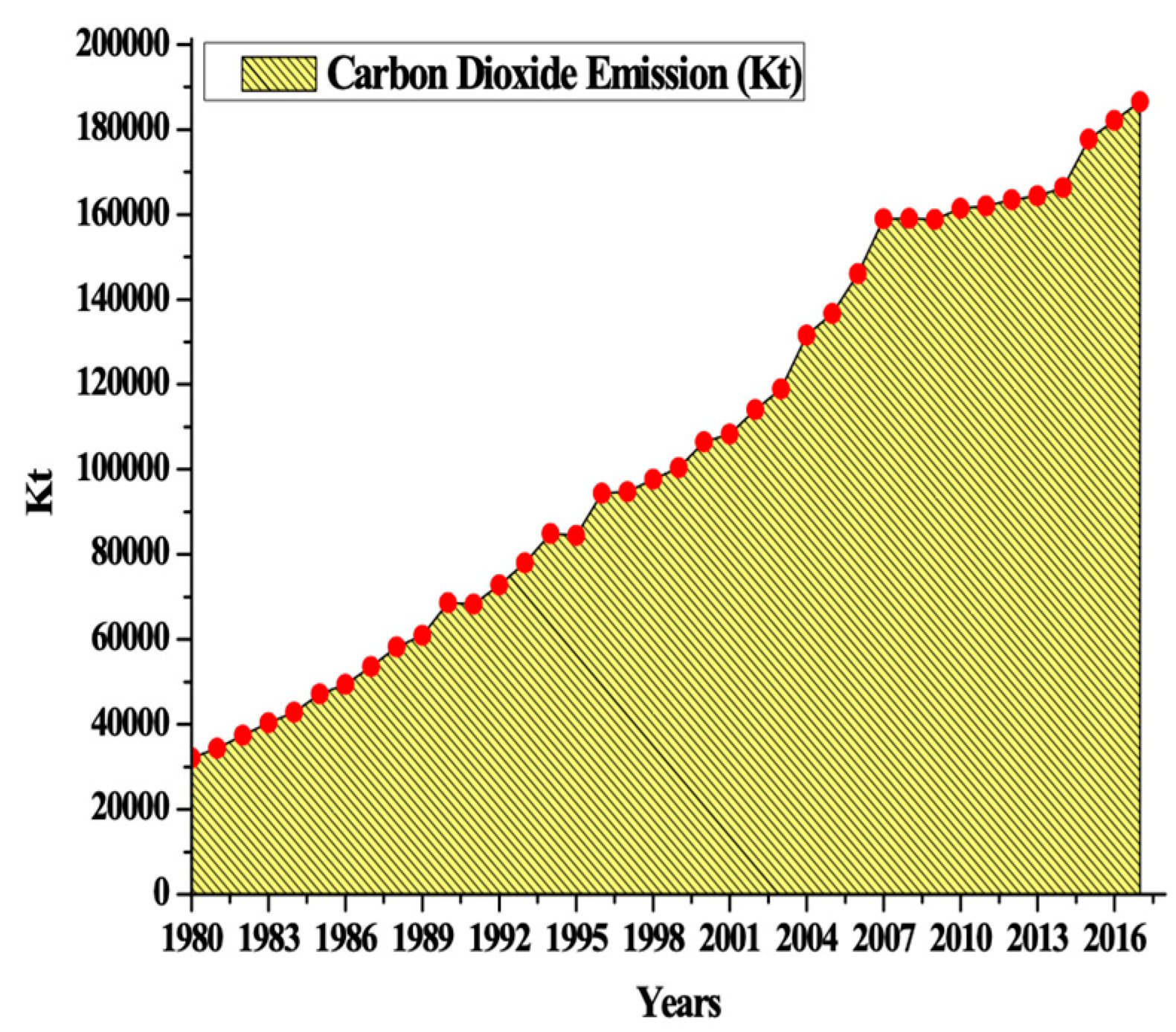
| CO2e | Carbon dioxide emission (kt) | WDI |
| CA | Cropped Area (Million Hectares) | GOP |
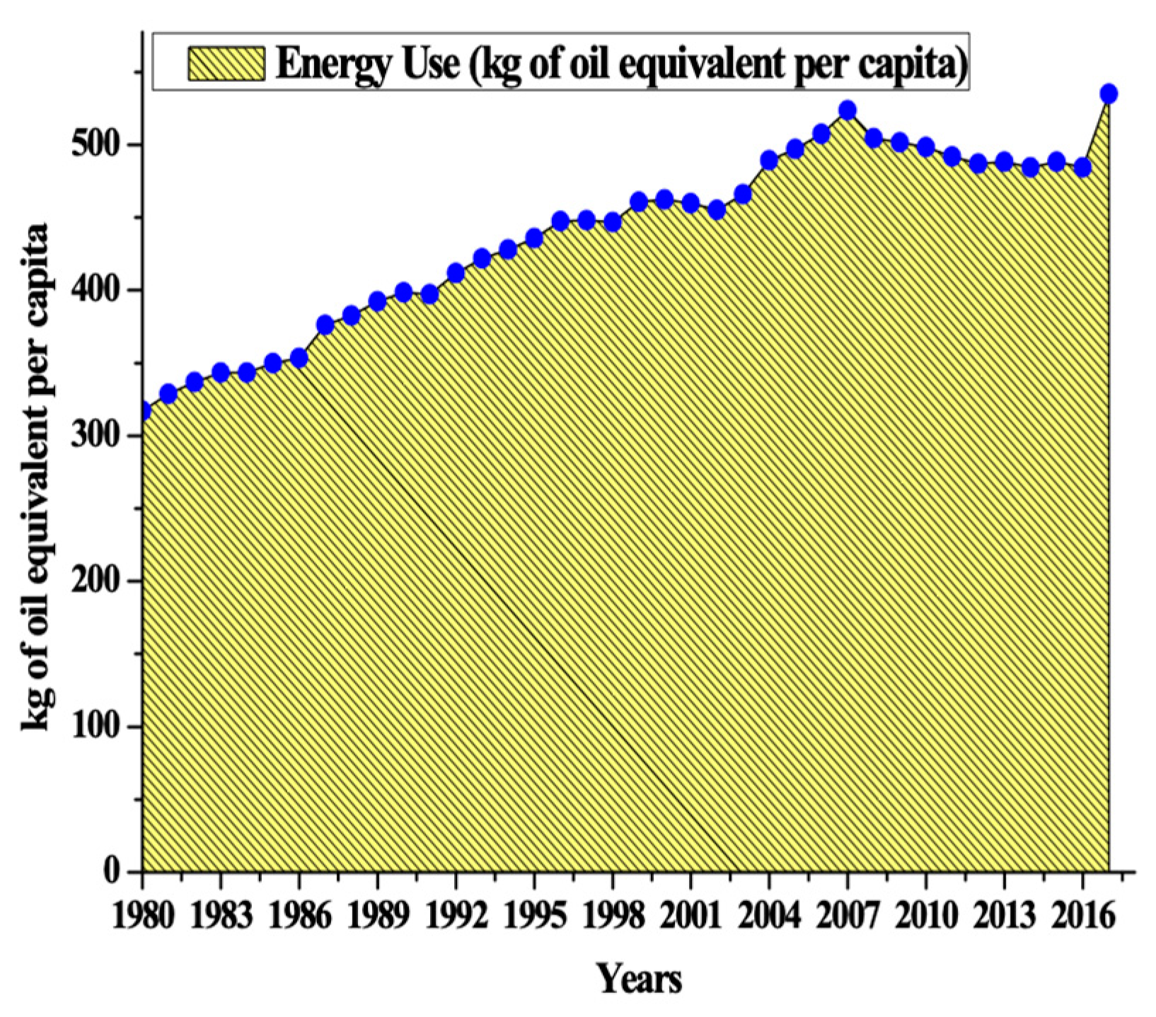
| EN | Energy Use (kg of oil equivalent per capita) | GOP |
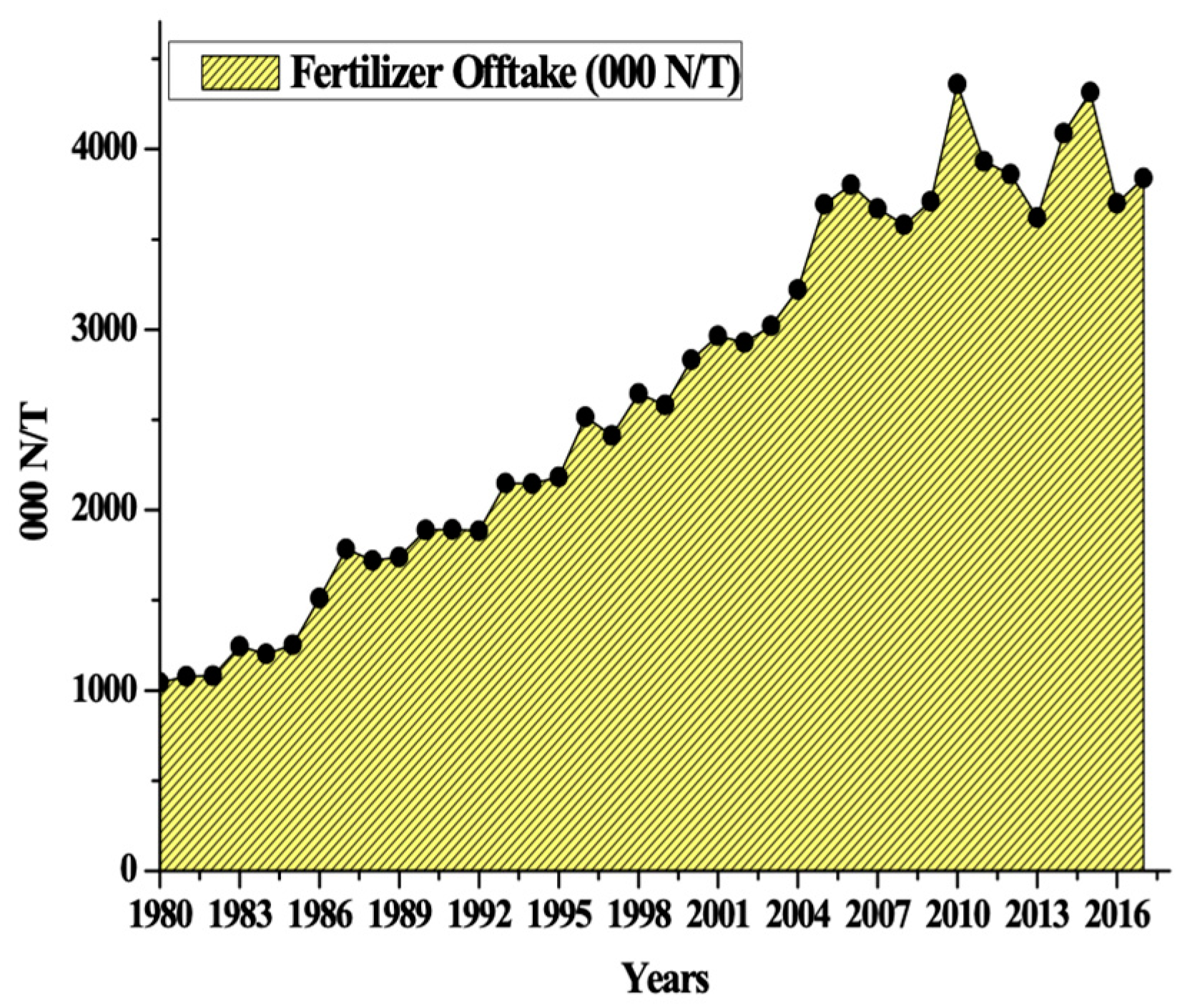
| FO | Fertilizer Offtake (N/T) | GOP |
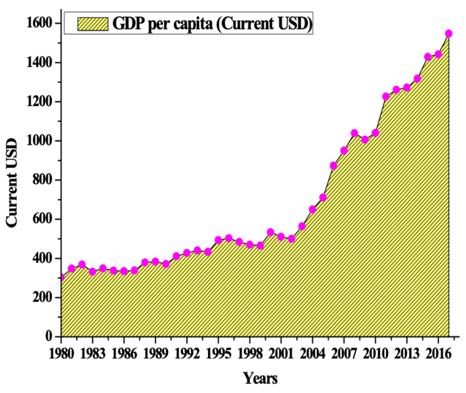
| GDPPC | GDP per capita (current USD) | WDI |
| ISD | Improved Seed Distribution (tons) | GOP |
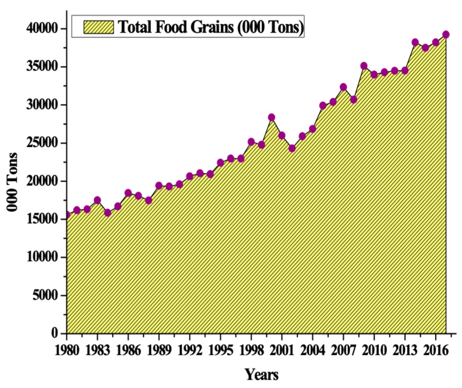
| TF | Total Food Grains (tons) | GOP |
| WA | Water Availability (MAF) | GOP |
| Variables | LNCO2e | LNCA | LNEN | LNFO | LNGDPPC | LNISD | LNTF | LNWA |
|---|---|---|---|---|---|---|---|---|
| Mean | 11.62931 | 3.272286 | 6.127777 | 7.960351 | 6.509023 | 5.129763 | 10.19537 | 4.866836 |
| Median | 11.64469 | 3.124125 | 6.136581 | 7.994980 | 6.280138 | 5.186100 | 10.16531 | 4.892452 |
| Maximum | 12.13631 | 4.144583 | 6.282379 | 8.380340 | 7.344624 | 6.175867 | 10.57740 | 4.931520 |
| Minimum | 10.88808 | 3.025291 | 5.929937 | 7.450080 | 5.826250 | 4.105120 | 9.768298 | 4.697932 |
| Std.Dev. | 0.379787 | 0.366298 | 0.095564 | 0.303646 | 0.492566 | 0.667094 | 0.248322 | 0.065605 |
| Skewness | −0.367964 | 1.827603 | −0.538492 | −0.328698 | 0.367273 | −0.144394 | −0.046627 | –1.230197 |
| Kurtosis | 1.875204 | 4.427214 | 2.289894 | 1.704256 | 1.596638 | 1.764649 | 1.735385 | 3.361083 |
| Jarque-Bera | 2.333727 | 19.88839 | 2.149521 | 2.726867 | 3.240772 | 2.078926 | 2.076932 | 7.987565 |
| Probability | 0.311342 | 0.000048 | 0.341380 | 0.255781 | 0.197822 | 0.353645 | 0.353997 | 0.018430 |
| Observations | 31 | 31 | 31 | 31 | 31 | 31 | 31 | 31 |
| LNCO2e | 1.000000 | |||||||
| LNCA | 0.287692 | 1.000000 | ||||||
| LNEN | 0.960217 | 0.195537 | 1.000000 | |||||
| LNFO | 0.980246 | 0.233428 | 0.945762 | 1.000000 | ||||
| LNGDPPC | 0.940177 | 0.365944 | 0.845598 | 0.908828 | 1.000000 | |||
| LNISD | 0.946856 | 0.380386 | 0.869403 | 0.945105 | 0.927329 | 1.000000 | ||
| LNTF | 0.976124 | 0.304974 | 0.915322 | 0.961370 | 0.962135 | 0.953546 | 1.000000 | |
| LNWA | 0.875045 | 0.080978 | 0.899151 | 0.862026 | 0.715330 | 0.768892 | 0.799829 | 1.000000 |
| Variable | ADF Test Statistics (at Levels) | ADF Test Statistics (at First Difference) | (Status) |
|---|---|---|---|
| LNCO2e | 0.947208 | −4.057989 ** | I(1) |
| LNCA | −3.465301 * | - | I(0) |
| LNEN | −1.999591 | −3.345375 * | I(1) |
| LNFO | 0.626924 | −5.871416 *** | I(1) |
| LNGDPPC | −1.592687 | −5.045839 *** | I(1) |
| LNISD | −3.446940 * | - | I(0) |
| LNTF | −4.780429 *** | - | I(0) |
| LNWA | −2.294522 | −8.244225 *** | I(1) |
| Variable | P-P Test Statistics (at Levels) | P-P Test Statistics (at First Difference) | (Status) |
|---|---|---|---|
| LNCO2e | −1.486801 | −6.911246 *** | I(1) |
| LNCA | −3.465301 * | - | I(0) |
| LNEN | −2.034168 | −3.345375 * | I(1) |
| LNFO | −1.849628 | −9.749996 *** | I(1) |
| LNGDPPC | −1.646333 | −5.041999 *** | I(1) |
| LNISD | −3.429725 * | - | I(0) |
| LNTF | −4.738381 *** | - | I(0) |
| LNWA | −1.955929 | −19.51462 *** | I(1) |
| F-Statistic | Significance Levels | Lower Bound | Upper Bound | Status |
|---|---|---|---|---|
| 3.870465 | 10 percent | 2.03 | 3.13 | Co-integrated |
| 5 percent | 2.32 | 3.50 | ||
| 1 percent | 2.96 | 4.26 |
| Null Hypothesis | Trace Test Statistic | P-value | Null Hypothesis | Maximum Eigenvalue | P-value |
|---|---|---|---|---|---|
| r ≤ 0 | 232.7068 * | 0.0000 | r ≤ 0 | 77.65021 * | 0.0000 |
| r ≤ 1 | 155.0566 * | 0.0002 | r ≤ 1 | 48.54521 | 0.0278 |
| r ≤ 2 | 106.5114 * | 0.0074 | r ≤ 2 | 31.58198 | 0.3264 |
| r ≤ 3 | 74.92944 * | 0.0184 | r ≤ 3 | 33.87687 | 0.1492 |
| r ≤ 4 | 45.33503 | 0.0846 | r ≤ 4 | 27.58434 | 0.0798 |
| r ≤ 5 | 19.38669 | 0.4654 | r ≤ 5 | 21.13162 | 0.5728 |
| r ≤ 6 | 7.639644 | 0.5047 | r ≤ 6 | 14.26460 | 0.8568 |
| Dependent variable is lnCO2e: ARDL(1, 1, 0, 1, 1, 0, 0, 1) selected based on AIC | ||||
|---|---|---|---|---|
| Panel A: long-run Analysis | ||||
| Variable | Coefficient | Std. Error | T- Ratio | P-value |
| LNCA | 0.072391 | 0.026865 | 2.694625 | 0.0148 |
| LNEN | 0.826146 | 0.241722 | 3.417754 | 0.0031 |
| LNFO | 0.607328 | 0.136929 | 4.435357 | 0.0003 |
| LNGDPPC | 0.211959 | 0.054088 | 3.918779 | 0.0010 |
| LNISD | −0.042691 | 0.041699 | −1.023784 | 0.3195 |
| LNTF | −0.031709 | 0.158234 | −0.200393 | 0.8434 |
| LNWA | 0.706882 | 0.245003 | 2.885204 | 0.0099 |
| C | −2.742992 | 1.074045 | −2.553890 | 0.0199 |
| Panel B: Short-run Analysis | ||||
| LNCA | 0.031187 | 0.015035 | 2.074271 | 0.0527 |
| LNEN | 0.615764 | 0.203512 | 3.025696 | 0.0073 |
| LNFO | 0.312632 | 0.088522 | 3.531681 | 0.0024 |
| LNGDPPC | −0.046796 | 0.078172 | −0.598633 | 0.5569 |
| LNISD | −0.031819 | 0.030053 | −1.058762 | 0.3037 |
| LNTF | −0.023634 | 0.116811 | −0.202329 | 0.8419 |
| LNWA | 0.206519 | 0.209902 | 0.983881 | 0.3382 |
| ECM (−1) | −0.745345 | 0.136764 | −5.449872 | 0.0000 |
| Panel C. Residual Diagnostic Test | ||||
| R-squared 0.997706 | ||||
| Adjusted R-squared 0.996086 | ||||
| Durbin-Watson stat 2.698081 | ||||
| F-statistic 16.0557*** | ||||
| χ2 SERIAL | 1.7655 (0.202) | |||
| χ2 NORMAL | 0.0724 (0.964) | |||
| χ2ARCH | 0.1557 (0.696) | |||
| χ2 RESET | 0.7142 (0.48) | |||
© 2019 by the authors. Licensee MDPI, Basel, Switzerland. This article is an open access article distributed under the terms and conditions of the Creative Commons Attribution (CC BY) license (http://creativecommons.org/licenses/by/4.0/).
Share and Cite
Rehman, A.; Ozturk, I.; Zhang, D. The Causal Connection between CO2 Emissions and Agricultural Productivity in Pakistan: Empirical Evidence from an Autoregressive Distributed Lag Bounds Testing Approach. Appl. Sci. 2019, 9, 1692. https://doi.org/10.3390/app9081692
Rehman A, Ozturk I, Zhang D. The Causal Connection between CO2 Emissions and Agricultural Productivity in Pakistan: Empirical Evidence from an Autoregressive Distributed Lag Bounds Testing Approach. Applied Sciences. 2019; 9(8):1692. https://doi.org/10.3390/app9081692
Chicago/Turabian StyleRehman, Abdul, Ilhan Ozturk, and Deyuan Zhang. 2019. "The Causal Connection between CO2 Emissions and Agricultural Productivity in Pakistan: Empirical Evidence from an Autoregressive Distributed Lag Bounds Testing Approach" Applied Sciences 9, no. 8: 1692. https://doi.org/10.3390/app9081692