Perforated Medium Applied in Frequency Selective Surfaces and Curved Antenna Radome

Abstract

A perforated medium (PM) combined with an ultra-wideband frequency selective surface (FSS) is proposed for the antenna radome design, which provides more flexibility in the radome materials selection and processing. The dielectric constant performance of the PM can be improved by perforating air holes through the medium, thus the restrictions of the FSS medium material parameters can be released. A multiscale homogenization method is utilized to calculate the dielectric constant of this PM, and the transmission coefficients of the planar FSS structure at different incidence angles are computed. The PM FSS is then applied in the curved antenna radome. The physical optic method serves to analyze the transmission performance of the curved antenna radome. In order to reduce the computational difficulties and meet the requirements of physical optic computing, the transmission coefficients are obtained as a function of the frequency by the vector fitting method, and the incidence angle dependence is deduced by B spline interpolation. The simulated and experimental radiation patterns with and without the radome are compared and the results show good agreement.

1. Introduction

The curved frequency selective surface (FSS) structure has many potential engineering application prospects. To the antenna radome, generally, there are some special requirements for the FSS radome materials. On the other hand, the FSS structure needs to meet certain specifications to have satisfactory performance. The ideal FSS is an infinite periodic surface structure composed of some basic elements, which have a frequency selective function for radiated electromagnetic waves and can be regarded as a spatial filter. After decades of research, the structure and performance of FSS have been improved in many aspects. The existing prefabricated mediums have many dielectric constant values to be used in a variety of FSS designs, which are mainly distributed in 2.2 to 10.2 [1,2,3,4,5,6,7]. The ultra-wideband properties of FSS are closely related to the periodic element structure, dielectric material property and FSS layer structure. In curved and ultra-wideband FSS cell designs, the interwoven convoluted structure can reduce the cell size and increase the bandwidth [7]. Reference [8] proposed an ultra-wideband FSS and its 3 dB bandwidth reached 12.6 GHz (5.85–18.45 GHz) at vertical incidence angle, the structure consists of three FSS patches and two 1 mm medium layers. In warped FSS, the bandwidths of different incident angles are a very important index. The planar FSS in reference [8] had a good technical performance within the 30° incident angle. However, this type of structure had an exacting requirement on its medium electromagnetic property. Generally speaking, a wider FSS bandwidth requires a lower medium dielectric constant, thus, there is a significant increase in costs. In terms of this issue, a method of air holes perforated through the normal medium to decrease the equivalent dielectric constant value is proposed in this paper, thus an ultra-wideband FSS can be accomplished with cheaper and lighter materials.

With air through holes through the medium, the medium macroscopic dielectric constant value is obviously altered. Several methods were put forward to obtain the mixed medium dielectric constant, the effective medium theory included. These methods function by being able to define averages that hope to be representative of the system and be connected with experimental measurements in the macroscopic situation. Thus, providing the basis for the widely used Maxwell–Garnett formula [9,10]. The modern homogenization theory is an effective method to obtain the composite dielectric constant, the multiscale homogenization method was proposed afterwards [11,12,13,14,15,16,17]. The effective dielectric constant of the perforated medium (PM) is computed by the multiscale method, in which the microscale field in the period unit is computed, and the macro parameters are obtained by the average of the microscale field. The results of the multiscale method can be compared with the non-perforated medium FSS, and the performances of the FSSs can be calculated.

The curved FSS radome can be developed based on the PM FSS performance obtained above. In practice, the FSS needs to form a corresponding curved surface structure according to different application systems, such as the antenna reflective surface and cover, and some are oversized. Based on the application environment of the curved FSS radome, an accurate calculation method is needed to calculate the transmission coefficients of different frequencies and incident angles [18,19,20]. This paper adopts the vector fitting method to fit the planar FSS transmission coefficients as the function of frequency. The FSS transmission coefficients functions of different incident angles then utilize B spline interpolation to reduce the data size. The transmission coefficients functions are synthesized base on the physical optic method to analyze the curved FSS transmission coefficients.

The physical optic method is adopted on account of at least two problems encountered when we calculate and analyze the performance of electrically large nonplanar structure: (1) The planar Floquet model in simulation software’s cannot be applied in curved surface simulations; (2) the existing electromagnetic fields full wave analysis methods require huge computing resources and lengthy computing time in composite electrically large structures. To an electrically large radome, the ray method is employed to obtain the incident angle of every point on the radome surface, thus the radome transmission coefficients could be computed at these points using these incident angles [21,22]. The physical optic method was chosen in reference [23] and it was also utilized in the curved FSS radome in references [24,25]. According to all the available studies, the high frequency method is a very effective way to analyze a curved electrically large surface, the calculation and analysis results can reach the same accuracy compared to the experiments [26]. Eventually, the radiation patterns with and without the radome are compared and reach a good agreement.

2. Planar Ultra-Wideband FSS Design

FSS usually uses a dielectric plate as the structural support of the planar unit. Study results show that high performance FSS relied on not only excellent structural design, but also its high-performing medium. Reference [6] proposed a grid square structure FSS, which can reach a broad bandwidth, but many medium parameters were not mentioned. Reference [8] used a high cost dielectric medium plate with a relative dielectric constant of 2.65 and 2 mm thickness to accomplish the FSS in reference [6], but merits of low profile, flat passband, and stable performance for different polarizations and various incident angles within 30° are achieved. These works are remarkable, but it will be highly valued in practical applications if low-cost materials can be promoted to a superior performance and realize wideband FSS.

The PM proposed in this paper is a composite medium structure and can meet the requirement of wideband. Furthermore, the total weight and fabricating cost of huge radome can be significantly decreased by air through holes. The frequently-used material with a relative dielectric constant of 4.4 is adopted in this article. Using the through holes structure, a 2.70 equivalent dielectric constant can be obtained and an FSS structure is shown in Figure 1. The structure is partially optimized base on references [6,8], both the processing difficulties and FSS performance have been taken into consideration for the geometric dimensions. There are four perforations through each FSS periodic unit medium, which aim to reduce the equivalent dielectric constant of the dielectric plate and decrease the weight, red cylinders in Figure 1 are the air through holes. The top and bottom layers are the same metallic patches, shown as the blue patches in Figure 1. The middle layer is a square metallic grid shown as the yellow part. The unit is a 4 × 4 mm² square with the following values: h = 2 mm, w = 2 mm, a = 0.5 mm, b = 0.5 mm, d = 1 mm.

With the blueprint of the PM structure and FSS frame, a detailed investigation of the dielectric constant of the PM FSS must be performed. The multiscale homogenization method is utilized in this paper for the numeric analysis of the PM dielectric constant. The solutions of the multiscale problems are obtained by solving the multiscale equations respectively [16,17]. When applying the Maxwell equations to the composite structure multiscale problems solving, there are:

$$\{\begin{array}{c}j\omega \epsilon \mathit{E} = \nabla \times \mathit{H}\\ j\omega \mu \mathit{H} = -\nabla \times \mathit{E}\end{array},$$

(1)

and the electric field vector in passive region follows:

$$\nabla \times \frac{1}{\mu }\nabla \times \mathit{E}-{\omega }^2\epsilon \mathit{E} = 0.$$

(2)

In multiscale problems, $\xi$ represents a microscale variable, and $x$ represents a large-scale variable. The electric field of multiscale problem can be resolved into the average field and microscale field:

$$\mathit{E}\left(x,\xi \right) = \mathit{E}\left(x\right)+\mathit{A}\left(x,\xi \right),$$

(3)

where $\mathit{A}\left(x,\xi \right)$ is the correction term in small scale and is an arbitrary vector field which can be applied to situations of both rotational field and divergence field. Substituting Equation (3) into Equation (2):

$$\nabla \times \nabla \times \left[\mathit{E}\left(x\right)+\mathit{A}\left(x,\xi \right)\right]-k^2{\epsilon }_r\left[\mathit{E}\left(x\right)+\mathit{A}\left(x,\xi \right)\right] = 0,$$

(4)

where $k^2={\omega }^2{\epsilon }_0\mu$. According to the derivative operation, there is:

$$\begin{array}{ll}\nabla \times \nabla \times \left[\mathit{E}\left(x\right)+\mathit{A}\left(x,\xi \right)\right]& = \nabla \times \left\{{\nabla }_x\times \left[\mathit{E}\left(x\right)+\mathit{A}\left(x,\xi \right)\right]+\frac{1}{a}{\nabla }_{\xi }\times \left[\mathit{E}\left(x\right)+\mathit{A}\left(x,\xi \right)\right]\right\}\\ & = {\nabla }_x\times \left\{{\nabla }_x\times \left[\mathit{E}\left(x\right)+\mathit{A}\left(x,\xi \right)\right]+\frac{1}{a}{\nabla }_{\xi }\times \left[\mathit{E}\left(x\right)+\mathit{A}\left(x,\xi \right)\right]\right\}\\ & +\frac{1}{a}{\nabla }_{\xi }\times \left\{{\nabla }_x\times \left[\mathit{E}\left(x\right)+\mathit{A}\left(x,\xi \right)\right]+\frac{1}{a}{\nabla }_{\xi }\times \left[\mathit{E}\left(x\right)+\mathit{A}\left(x,\xi \right)\right]\right\},\end{array}$$

(5)

where $a$ is the periodic unit length of the composite structure. Consider a non-magnetic-conducting material and Equation (5) can be reduced to:

$${\nabla }_x\times {\nabla }_x\times \mathit{E}\left(x\right)+\frac{1}{a^2}{\nabla }_{\xi }\times {\nabla }_{\xi }\times \mathit{A}\left(x,\xi \right)-k^2{\epsilon }_r\left[\mathit{E}\left(x\right)+\mathit{A}\left(x,\xi \right)\right] = 0.$$

(6)

The first order approximate equation of the macro-scale fields is:

$${\nabla }_x\times {\nabla }_x\times \mathit{E}\left(x\right)-k^2\mathit{E}\left(x\right) = 0,$$

(7)

thus Equation (6) can be simplified:

$$\frac{1}{a^2}{\nabla }_{\xi }\times {\nabla }_{\xi }\times \mathit{A}\left(x,\xi \right)-k^2{\epsilon }_r\left[\mathit{E}\left(x\right)+\mathit{A}\left(x,\xi \right)\right] = -k^2\mathit{E}\left(x\right).$$

(8)

Take the inner product of vector weight function $\mathit{w}$ and Equation (6) in the space periodic unit $\mathsf{\Omega }$:

$$\underset{\mathsf{\Omega }}{{\displaystyle \iiint }}\left\{{\nabla }_{\xi }\times {\nabla }_{\xi }\times \mathit{A}\left(x,\xi \right)-k^2{a}^2{\epsilon }_r\left[\mathit{E}\left(x\right)+\mathit{A}\left(x,\xi \right)\right]\right\}·\mathit{w}·dv = -\underset{\mathsf{\Omega }}{{\displaystyle \iiint }}{k}^2{a}^2\mathit{E}\left(x\right)·\mathit{w}·dv.$$

(9)

Define:

$$\{\begin{array}{c}{\mathit{A}}^x\left(x,\xi \right)= E_x\left(x\right)·{\mathit{A}}_1^x\left(x,\xi \right)\\ {\mathit{A}}^y\left(x,\xi \right)= E_y\left(x\right)·{\mathit{A}}_1^y\left(x,\xi \right)\\ {\mathit{A}}^z\left(x,\xi \right)= E_z\left(x\right)·{\mathit{A}}_1^z\left(x,\xi \right)\end{array}.$$

(10)

The microscale functional equations about $\mathit{A}$ is obtained where $\widehat{x}$, $\widehat{y}$, and $\widehat{z}$ are the unit vectors:

$$\{\begin{array}{l}\langle {\nabla }_{\xi }\times {\mathit{A}}_1^x\left(x,\xi \right),{\nabla }_{\xi }\times \mathit{w}\left(\xi \right)\rangle -\langle k^2{\epsilon }_r{a}^2·\left[\widehat{x}+{\mathit{A}}_1^x\left(x,\xi \right)\right],\mathit{w}\left(\xi \right)\rangle +\langle k^2{a}^2\widehat{x},\mathit{w}\left(\xi \right)\rangle = 0\\ \langle {\nabla }_{\xi }\times {\mathit{A}}_1^y\left(x,\xi \right),{\nabla }_{\xi }\times \mathit{w}\left(\xi \right)\rangle -\langle k^2{\epsilon }_r{a}^2·\left[\widehat{y}+{\mathit{A}}_1^y\left(x,\xi \right)\right],\mathit{w}\left(\xi \right)\rangle +\langle k^2{a}^2\widehat{y},\mathit{w}\left(\xi \right)\rangle = 0\\ \langle {\nabla }_{\xi }\times {\mathit{A}}_1^z\left(x,\xi \right),{\nabla }_{\xi }\times \mathit{w}\left(\xi \right)\rangle -\langle k^2{\epsilon }_r{a}^2·\left[\widehat{z}+{\mathit{A}}_1^z\left(x,\xi \right)\right],\mathit{w}\left(\xi \right)\rangle +\langle k^2{a}^2\widehat{z},\mathit{w}\left(\xi \right)\rangle = 0\end{array}$$

(11)

The microscale solution is obtained based on Equations (9) and (11), which can express the total field solution in composite structure as:

$$\begin{array}{ll}\mathit{E}\left(x,\xi \right)& = \mathit{E}\left(x\right)+\mathit{A}= \mathit{E}\left(x\right)+E_x\left(x\right){\mathit{A}}_1^x+E_y\left(x\right){\mathit{A}}_1^y+E_z\left(x\right){\mathit{A}}_1^z\\ & = E_x\left(x\right)[x+{\mathit{A}}_1^x\left]+E_y\left(x\right)\right[y+{\mathit{A}}_1^y\left]+E_z\left(x\right)[z+{\mathit{A}}_1^z\right].\end{array}$$

(12)

Take the average of the integral of Equation (6) in periodic unit, then the homogenization field equation is:

$${\nabla }_x\times {\nabla }_x\times \mathit{E}\left(x\right)-{\omega }^2{\mu }_0{\epsilon }_0{\stackrel{\rightharpoonup }{\overrightarrow{\epsilon }}}_{eff}\mathit{E}\left(x\right) = 0.$$

(13)

where the effective dielectric constant ${\stackrel{\rightharpoonup }{\overrightarrow{\epsilon }}}_{eff}$ can be expressed as:

$$\{\begin{array}{l}{\epsilon }_{xx}= \underset{\mathsf{\Omega }}{{\displaystyle \iiint }}\epsilon \left(\xi \right)\left(1+A_{1x}^x\right)d\mathsf{\Omega }\\ {\epsilon }_{xy}= \underset{\mathsf{\Omega }}{{\displaystyle \iiint }}\epsilon \left(\xi \right)A_{1x}^{y}d\mathsf{\Omega }\\ {\epsilon }_{xz}= \underset{\mathsf{\Omega }}{{\displaystyle \iiint }}\epsilon \left(\xi \right)A_{1x}^{z}d\mathsf{\Omega }\end{array},$$

(14)

$$\{\begin{array}{l}{\epsilon }_{yx}= \underset{\mathsf{\Omega }}{{\displaystyle \iiint }}\epsilon \left(\xi \right)A_{1y}^{x}d\mathsf{\Omega }\\ {\epsilon }_{yy}= \underset{\mathsf{\Omega }}{{\displaystyle \iiint }}\epsilon \left(\xi \right)(1+A_{1y}^y)d\mathsf{\Omega } \\ {\epsilon }_{yz}= \underset{\mathsf{\Omega }}{{\displaystyle \iiint }}\epsilon \left(\xi \right)A_{1y}^{z}d\mathsf{\Omega }\end{array},$$

(15)

$$\{\begin{array}{l}{\epsilon }_{zx}= \underset{\mathsf{\Omega }}{{\displaystyle \iiint }}\epsilon \left(\xi \right)A_{1z}^{x}d\mathsf{\Omega }\\ {\epsilon }_{zy}= \underset{\mathsf{\Omega }}{{\displaystyle \iiint }}\epsilon \left(\xi \right)A_{1z}^{y}d\mathsf{\Omega }\\ {\epsilon }_{zz}= \underset{\mathsf{\Omega }}{{\displaystyle \iiint }}\epsilon \left(\xi \right)(1+A_{1z}^z)d\mathsf{\Omega }\end{array}.$$

(16)

It is shown from Equations (1) to (16) that the calculated effective dielectric constant of the homogenization field is composed of two parts: (1) The dielectric constant of the background material and the dopant material, while in this paper they are FR4 and perforated air through holes, respectively; (2) vector field correction term $\mathit{A}\left(x,\xi \right)$, which is related to the frequency. References [16,17] utilized the gradient of the scalar potential function as the correction term in the small scale. However, when this correction term is used in the metamaterial studies, the equivalent electromagnetic parameters are only influenced by quasi-static field, the contribution of the rotational field is not involved. In terms of this issue, this paper introduces vector field correction term into consideration, thus, both divergence field and rotational field are involved. Furthermore, in comparison with the traditional Maxwell-Garnett theory, which homogenizes the dielectric constant to a constant value, this multiscale homogenization method can reveal the dielectric constant variation related with frequency.

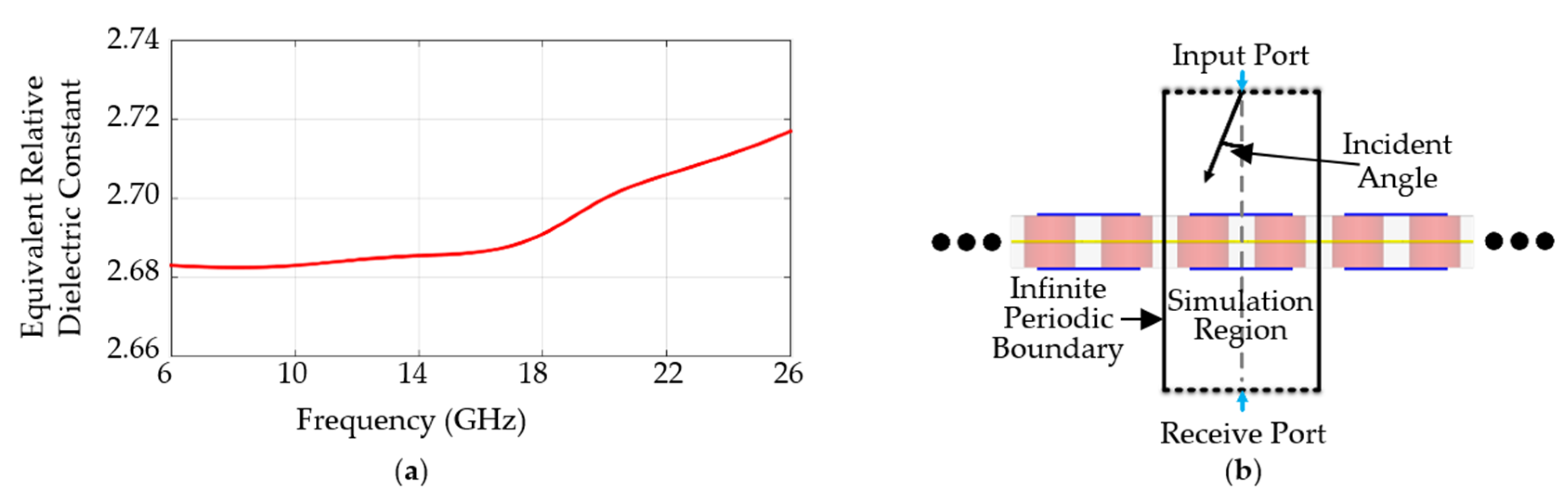
Based on the above theory, the electromagnetic parameters of the periodic units can be calculated. The equivalent relative dielectric constant of the PM FSS structure in Figure 1 is shown in Figure 2a. This curve states that the medium has an effective dielectric constant which changes in the 2.68 to 2.72 range within 6 to 25 GHz. The change in value is the effect of the vector field correction term related to the frequency. The variation is small because of the thin FSS unit thickness and the relatively simple background. The slight dielectric constant variation has little impact on the radome manufacture, even the process specification of distinguished corporation may have a 0.05 relative dielectric constant variation [27].

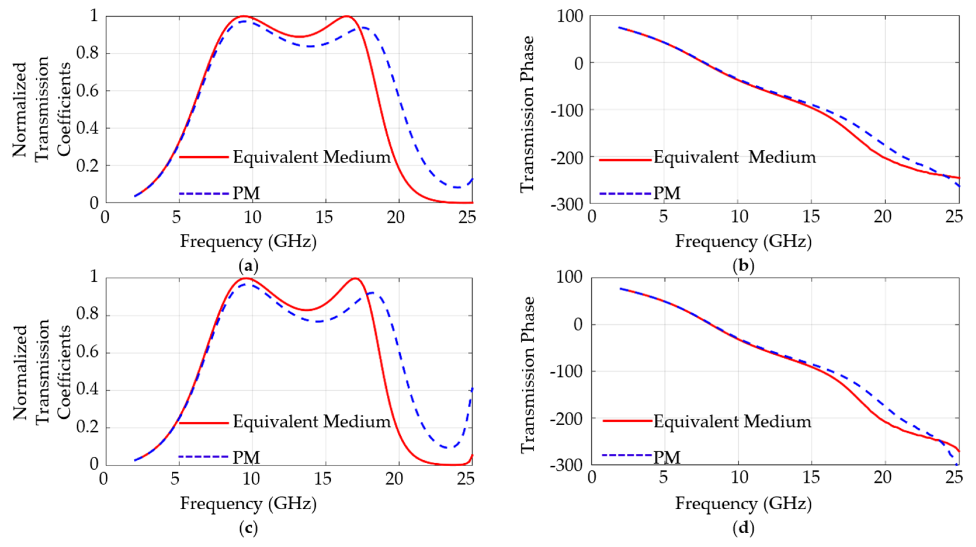
The FSS unit is simulated using the Finite Element Method (FEM) method in the infinite periodic structure, as shown in Figure 2b. The simulated transmission coefficients result of the transverse electric (TE) incident wave through the planar FSS surfaces are shown in Figure 3, where the equivalent medium means an equivalent 2.70 dielectric constant medium in the figure, and the transmission phase means the phase variation of the transmitted wave from the FSS unit upper surface to the lower surface. The two curves are the results of the equivalent 2.70 dielectric constant medium and the PM FSS, respectively, and the results of the 30° incident wave are also shown. From the comparison of the results, the two FSS with different media have very close transmission coefficients within the operating frequency range, especially the transmission coefficients phase. As far as the normalized transmission coefficients is concerned, transmission coefficients in the 2 to 8 GHz range are almost the same because the FSS is not in its working band, small dielectric constant variations can hardly change the transmission coefficients. In the 8 to 17 GHz range, the equivalent 2.70 dielectric constant medium has better transmission coefficient values because this FSS structure is intended for an ideal 2.70 dielectric constant, while the PM FSS dielectric constant is not equal to it, thus reducing the performance. And in the 17 to 25 GHz range, the wavelength of the incident wave gets much closer to the unit dimension and perforation size, thus more portions of the incident wave are transmitted through the FSS. The transmission phase curves have only minor differences for reason that the tiny change in dielectric constant value of the ultrathin FSS has little effect on the phase. A profound study on the periodic unit transmission performance is related to the transmission characteristics in the complex dielectric waveguide and some other theories and is not the main content of this paper.

The results of the transverse magnetic (TM) mode and other incident angles are comparable to Figure 3 and are omitted. The conventional FSS unit has a dimension about half of the resonant wavelength, and the bandwidth could not be very wide. Under this circumstance, the mode of the incident wave obviously affects the FSS transmission coefficients when the incident angle increases. However, the PM FSS structure proposed in this paper possesses a TE/TM insensitivity trait, which primarily comes from the unit periodicity, and is about only 1/10 wavelength of the lower passband. In such a small dimension, the FSS structure have negligible influence on the TE and TM incident wave, even when the incident angle increases. In the frequency range higher than 24 GHz, the transmission coefficients have distortions, the TE and TM mode transmission coefficients have significant changes. However, in this paper, the passband is approximately 7 to 17 GHz, where the TE/TM insensitivity trait of the PM FSS is obvious. In this way, the high transmissivity of an FSS, which has a 7 to 17 GHz ultra-wideband, is fulfilled. Depending on the validity of the high-end simulation software, the results above can certify the applicability of this PM FSS and can be applied to radome calculations.

3. Planar FSS Transmission Coefficient Vector Fitting

Before applying planar PM FSS to the curved radome, further data processing has to be accomplished. The PM FSS dielectric constant data of wide incident angles and broadband frequencies are too colossal and complicated, a direct computation based on the data may cause too much stagnation and cost too much time. A more effective way is to fit the transmission coefficients of the PM FSS as a function of frequency and incident angle. The vector fitting method is an efficient algorithm to adopt rational functions to approximate S parameters, the numerical results can be expressed as analytic functions using vector fitting. In high frequency analysis, the calculation of the radome transmission coefficients is very important but it is difficult to get the analytic expressions of the transmission coefficients in general. The numerical table lookup method requires a considerable amount of computation and a long calculation time. Vector fitting can approximate the analytic functions of the radome transmission coefficients, which will greatly simplify the complexity of analysis and calculation. To describe the relationship between the transmission coefficients and frequency, the rational fraction model, polynomial model, and partial fraction model can be used. In the vector fitting method, the partial fraction model and residues are utilized to approximate the variation relation of transmission coefficients and frequency [19]. Equation (17) shows a general expression of partial fractions:

$$f\left(s\right)= {\displaystyle \sum }_{j=1}^N\frac{c_j}{s-a_j}+d+e·s,$$

(17)

where $a_j$ is the complex pole, $c_j$ is the complex residue at the pole, $e$ and $d$ are real constants, and $s=j\omega$. If $a_j$ is known, the $1/(s-a_j)$ could be seen as a basic function, thus, the least squares method can be used to fit the data. However, in actual situations the poles are unknown and fitting the poles is necessary in order to practically fit the transmission coefficients data. To find the poles and residues, we begin with a set of starting poles $\left\{a_j\right\}$ and build the following functional expressions:

$$\sigma \left(s\right)f\left(s\right) = {\displaystyle \sum }_{n=1}^N\frac{c_n}{s-\overline{a_n}}+d+s·h,$$

(18)

$$\sigma \left(s\right) = {\displaystyle \sum }_{j=1}^N\frac{\widetilde{c_n}}{s-\overline{a_n}}+1.$$

(19)

Equation (19) multiplied by $f\left(s\right)$ leads to the following equation:

$${\displaystyle \sum }_{n=1}^N\frac{c_n}{s-\overline{a_n}}+d+s·h =\left({\displaystyle \sum }_{j=1}^N\frac{\widetilde{c_n}}{s-\overline{a_n}}+1\right)f\left(s\right).$$

(20)

A set of overdetermined equations contain the coefficients $c_n$, $d$, $h$, and $\widetilde{c_n}$ of different frequencies can be acquired, and the unknown coefficients can be obtained by the least squares method [18].

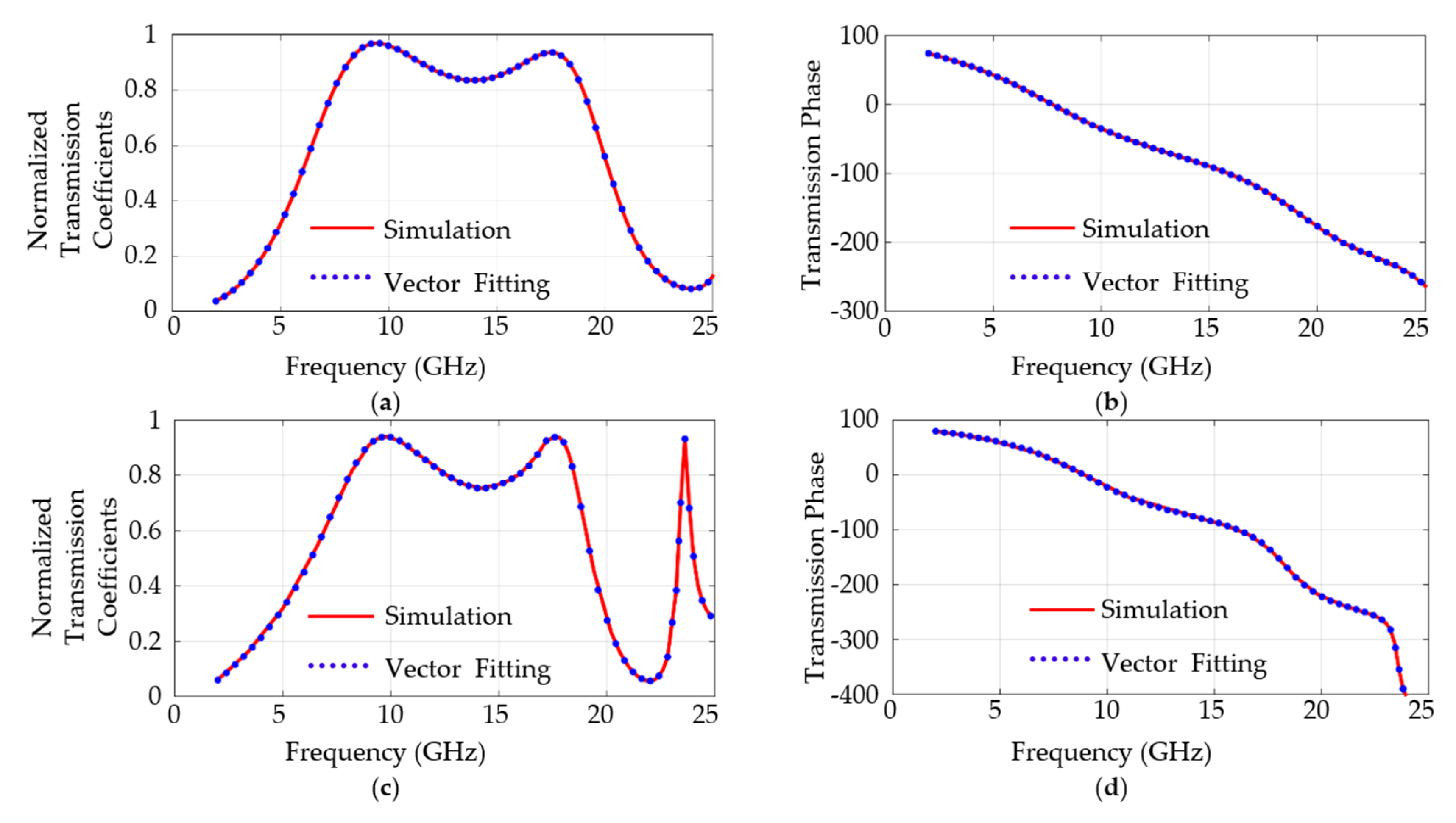
In order to study the influence of the different incident angles on the transmission coefficients, transmission coefficients functions at different incident angles are obtained by using the B spline interpolation method. In the vertical incident TE wave situation, six complex poles are used for vector fitting the transmission coefficients of PM FSS. The results are compared with the FEM simulations. Figure 4 shows that the vector fitting function and the numerical calculation results are consistent within 2 to 25 GHz in both vertical and 50° incident angle, which means that our method satisfies the requirements of high frequency analysis.

4. Curved Radome Physical Optic Analysis

The analysis of curved antenna radome can hardly be performed according to general computational electromagnetic full wave methods, because they are inefficient in solving electrically large problems. The high frequency methods can achieve fair precision in practical electrically large engineering problems. In the high frequency method, the physical optic method improves the computational accuracy compared to the geometric ray method. Thus, the usage of the physical optic method in this paper achieves a good balance between computational complexity and results accuracy. The main steps of analyzing the characteristics of the radome by the physical optic method are as follows:x

• Use the physical optic method to calculate the incident angle on the radome interior surface for the radome transmission coefficients computation;
• Obtain the transmitted field on the radome exterior surface by multiplying the incident field with radome transmission coefficients;
• Compute the antenna far field radiation by integrating the transmitted field on the radome exterior surface.

A radome surface is designed with a 1 m height and a bottom circle radius of 0.25 m, as shown in Figure 5. The radome exterior shape is described by the revolution of the curve $C$ rotated about the z axis, which satisfies the polynomial function relation:

$$C= A_0+A_{1}x+A_2{x}^2+A_3{x}^3+A_4{x}^4+A_5{x}^5,$$

(21)

where the polynomial coefficients are the fitting results of the radome from reference [26] and are shown in

Table 1. The polynomial coefficients of Equation (21).

$A_0$	$A_1$	$A_2$	$A_3$	$A_4$	$A_5$
0.2387	−1.203	34.63	−902.7	8912	−32,160

. The PM FSS partially cover the radome, as in Figure 5a the blue doubled imaginary line is shown. This partial coverage is for the measurement and fabrication convenience because only the upper space radiation patterns need to be considered. Ultimately, 19,488 periodic FSS units are needed for radome manufacture.

In the case with no radome, the radiation patterns of the horn antenna in the x polarization direction or y polarization direction with uniform current distribution can be calculated by the following formula:

$$E\left(\theta , \phi \right) = {\displaystyle \sum }_{m,n}{A}_{mn}\left(\theta , \phi \right)\exp \left[-j\left(ksin\left(\theta \right)\cos \left(\phi \right)x_{mn}+ksin\left(\theta \right)\cos \left(\phi \right)y_{mn}\right)\right].$$

(22)

With the radome influencing, the radiation patterns can be expressed as:

$$E_r = {\displaystyle \sum }_{m,n}{A}_{mn}\left(\theta , \phi \right)\left\{T\left(\theta , \phi \right)\exp \left[j\delta \left(\theta , \phi \right)\right]\right\}·\exp \left[-j\left(ksin\left(\theta \right)\cos \left(\phi \right)x_{mn}+ksin\left(\theta \right)\cos \left(\phi \right)y_{mn}\right)\right],$$

(23)

where $T\left(\theta , \phi \right)$ is the absolute radome transmission coefficients and $\delta \left(\theta , \phi \right)$ is the radome transmission coefficients phase.

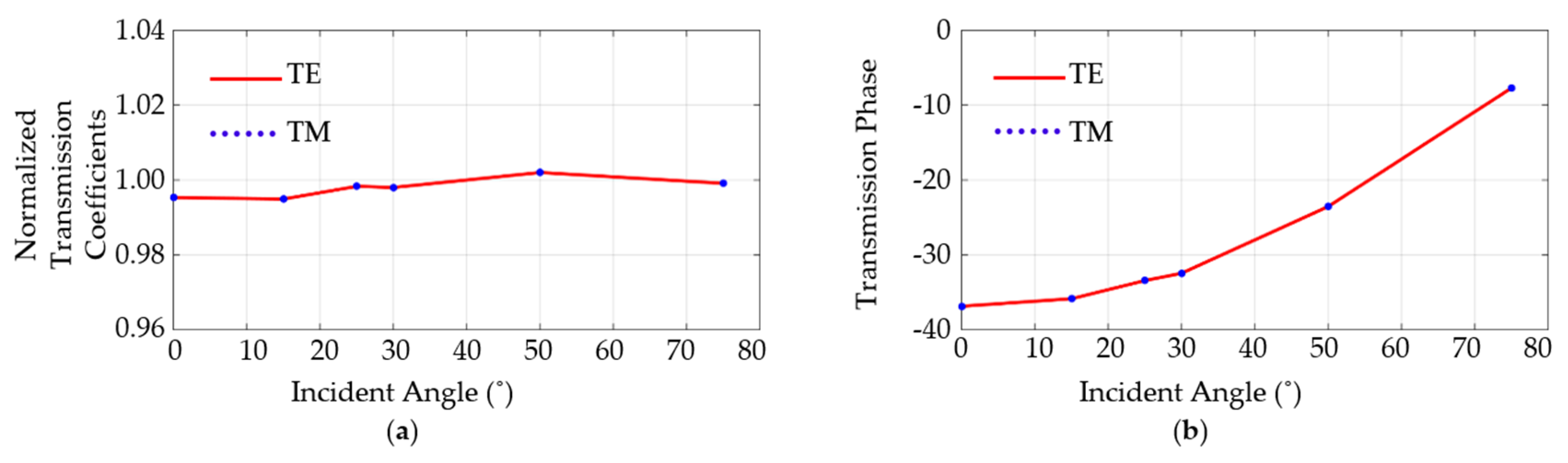
The radome transmission coefficients is closely linked to the incident angle. Figure 6 shows the 10 GHz planar PM FSS transmission coefficient curves of the TE and TM modes. Based on the theory described in Section 3, the FSS unit transmission coefficient will change accordingly with the change of incident angle. The data are collected at incident angles of 0, 15, 25, 30, 50 and 75°. As shown in the figure, the transmission coefficient range of the proposed FSS unit is close to 1 in both TE and TM modes but the transmission coefficient phase varies within the range of −6° to −37°. As discussed at the end of Section 3, the TE/TM insensitivity peculiarity of the PM FSS structure is verified again at 10 GHz. The 0 to 75° incident angle variation can affect the normalized transmission coefficients slightly. The larger incident angle may cause a longer propagation length, which will increase the phase difference. Apart from the incident angle variation, the discontinuity of the FSS could lead to the phase difference in the radome as well. With the radome covered, the difference of the antenna radiation field results from having different incident angles at the radome inner surface. Thus, the influence of the incident angles must be taken into consideration when calculating the total radiation diagram.

The physical optic method is adopted in order to consider the influence of different incident angles. Combining this method—the radome structure and horn antenna position—the incident angle at every point of the radome can be ascertained. Thus, the incident angle can be utilized to compute the small scale curved radome transmission coefficients, while considering the radome as a local plane. For each radiation direction, the intersection position of rays and the radome in the transmitting direction can be determined. At the intersection positions, the incident wave polarization is decomposed into a TM mode, which is parallel to the incident plane, and a TE mode, which is perpendicular to it. Multiplying these by the radome transmission coefficients and then synthesizing all the data, the radiation fields in the radiation direction are eventually acquired. Figure 7 shows the 10 GHz radiation patterns with and without the radome, the experimental results are also shown. The radome is experimented in the microwave anechoic chamber and a wideband highly directional horn antenna is fixed in the radome as shown in Figure 5a. The radome and the antenna are fastened to the rotation axis of the antenna automated test system in the chamber. Far field of the radiated electric field is received by another horn antenna. All the results are eventually compared in Figure 7 after data processing. Normalization of the data are not shown for the reason that the normalized curves overlap each other at both ends and cannot indicate the details.

It can be seen in Figure 7 that the experimental and simulated results agree well with each other. When the observing angle is within the range of −30° to 30°, the radiation patterns are in accord with each other, which reveals a high transmissivity in the vertical incident angle and nearby. Along with the observing angle increase, the transmitted field intensity decreases, which might be attributed to the physical optic method limitations.

5. Conclusions

A method for macroscale dielectric constant approximation has been investigated in this paper. Through holes are used to decrease the medium dielectric constant in the macroscale, and thus, materials with a low dielectric constant and high cost can be replaced by cheap PM. In this case, a 4.4 relative dielectric constant FR4 are perforated to have a medium dielectric constant of 2.70, with 20% weight lightened in each FSS unit, which will be significantly valuable in a practical antenna FSS radome design. With the usage of the multiscale homogenization method, the calculated relative dielectric constant of the PM is 2.70, adequately. The infinite periodic simulations of the FSS unit are carried out and the results of the 2.70 dielectric constant medium and the PM are compared. The results indicate that within 7 to 17 GHz range, the ultra-wideband PM FSS has a well approximated transmission coefficient compared with the 2.70 homogeneous dielectric constant medium. However, at frequencies above 22 GHz, there exists some difference between them. This conclusion is applicable to vertical incident TE waves, TM waves, and other incident angles.

If the transmission coefficients functions at each incident angle and frequency point of the planar FSS structure gained base on the vector fitting method and B spline interpolation, the characteristics of the curved radome can be analyzed. The FSS radome transmission coefficients are determined by considering the local curved radome as a plane in small scale. Thus, the radiation patterns with and without the FSS radome can be calculated by the physical optic method. The results show that the method presented here indicates a good prediction to the design of the curved radome performance.

References

- Anwar, R.S.; Mao, L.; Ning, H. Frequency Selective Surfaces: A Review. Appl. Sci. 2018, 8, 1689. [Google Scholar] [CrossRef]
- Munk, B.A. Frequency Selective Surfaces: Theory and Design; Wiley Online Library: Hoboken, NJ, USA, 2000; Volume 29, ISBN 0-471-37047-9. [Google Scholar]
- Glybovski, S.B.; Tretyakov, S.A.; Belov, P.A.; Kivshar, Y.S.; Simovski, C.R. Metasurfaces: From Microwaves to Visible. Phys. Rep. 2016, 634, 1–72. [Google Scholar] [CrossRef]
- Alibakhshikenari, M.; Nasermoghadasi, M.; Sadeghzadeh, R.A.; Virdee, B.S.; Limiti, E. Traveling-wave antenna based on metamaterial transmission line structure for use in multiple wireless communication applications. AEU Int. J. Electron. Commun. 2016, 70, 1645–1650. [Google Scholar] [CrossRef] [Green Version]
- Moharamzadeh, E. Radiation Characteristic Improvement of X-Band Slot Antenna Using New Multiband Frequency-Selective Surface. Int. J. Antenn. Propag. 2014, 2014, 321287. [Google Scholar] [CrossRef]
- Wu, T.K.; Verdes, R.P. Wideband Gridded Square Frequency Selective Surface. U.S. Patent Application No. 07/148312, 25 January 1988. [Google Scholar]
- Huang, F.; Batchelor, J.C.; Parker, E.A. Interwoven convoluted element frequency selective surfaces with wide bandwidths. Electron. Lett. 2006, 42, 788–790. [Google Scholar] [CrossRef] [Green Version]
- Zhou, H.; Qu, S.; Wang, J.; Lin, B.Q.; Ma, H.; Xu, Z.; Peng, W.D. Ultra-wideband frequency selective surface. Electron. Lett. 2012, 48, 11–13. [Google Scholar] [CrossRef]
- Choy, C.T. Effective Medium Theory: Principles and Applications, 2nd ed.; Oxford University Press: New York, NY, USA, 2016; pp. 27–55. ISBN 978–0–19–870509–3. [Google Scholar]
- Levy, O.; Stroud, D. Maxwell Garnett theory for mixtures of anisotropic inclusions: Application to conducting polymers. Phys. Rev. B 1997, 56, 8035–8046. [Google Scholar] [CrossRef]
- Tinga, W.R.; Voss, W.A.; Blossey, D.F. Generalized approach to multiphase dielectric mixture theory. J. Appl. Phys. 1973, 44, 3897–3902. [Google Scholar] [CrossRef]
- Bringi, V.N.; Varadan, V. Average dielectric properties of discrete random media using multiple scattering theory. IEEE Trans. Antenn. Propag. 1983, 31, 371–375. [Google Scholar] [CrossRef]
- Niyonzima, I.; Sabariego, R.V.; Dular, P.; Geuzaine, C. Finite Element Computational Homogenization of Nonlinear Multiscale Materials in Magnetostatics. IEEE Trans. Magn. 2012, 48, 587–590. [Google Scholar] [CrossRef] [Green Version]
- Hou, T.Y.; Wu, X. A Multiscale Finite Element Method for Elliptic Problems in Composite Materials and Porous Media. J. Comput. Phys. 1997, 134, 169–189. [Google Scholar] [CrossRef]
- Zeng, D.; Li, Y.; Lu, G. Study on multi-scale finite element method for EM wave equation. In Proceedings of the International Conference on Applications of Electromagnetism & Student Innovation Competition Awards, Taipei, China, 11–13 August 2010; pp. 19–23. [Google Scholar] [CrossRef]
- Ouchetto, O.; Zouhdi, S.; Bossavit, A.; Griso, G.; Miara, B. Modeling of 3-d periodic multiphase composites by homogenization. IEEE Trans. Microw. Theory 2006, 54, 2615–2619. [Google Scholar] [CrossRef]
- Ouchetto, O.; Qiu, C.W.; Zouhdi, S.; Li, L.W.; Razek, A. Homogenization of 3-d periodic bianisotropic metamaterials. IEEE Trans. Microw. Theory 2006, 54, 3893–3898. [Google Scholar] [CrossRef]
- Gustavsen, B.; Semlyen, A. Rational approximation of frequency domain responses by vector fitting. IEEE Trans. Power Deliv. 1999, 14, 1052–1061. [Google Scholar] [CrossRef]
- Gustavsen, B. Improving the pole relocating properties of vector fitting. IEEE Trans. Power Deliv. 2006, 21, 1587–1592. [Google Scholar] [CrossRef]
- Deschrijver, D.; Mrozowski, M.; Dhaene, T.; De Zutter, D. Macromodeling of multiport systems using a fast implementation of the vector fitting method. IEEE Microw. Wirel. Compon. 2008, 18, 383–385. [Google Scholar] [CrossRef]
- Paris, D. Computer-aided radome analysis. IEEE Trans. Antenn. Propag. 1970, 18, 7–15. [Google Scholar] [CrossRef]
- Einziger, P.D.; Felsen, L. Ray analysis of two-dimensional radomes. IEEE Trans. Antenn. Propag. 1983, 31, 870–884. [Google Scholar] [CrossRef]
- Moneum, M.A.; Shen, Z.; Volakis, J.L.; Graham, O. Hybrid PO-MoM analysis of large axi-symmetric radomes. IEEE Trans. Antenn. Propag. 2001, 49, 1657–1666. [Google Scholar] [CrossRef]
- Delia, U.F.; Pelosi, G.; Pichot, C.; Selleri, S.; Zoppi, M. A physical optics approach to the analysis of large frequency selective radomes. Prog. Electromagn. Res. 2013, 138, 537–553. [Google Scholar] [CrossRef]
- Kim, J.H.; Chun, H.J.; Hong, I.; Kim, Y.J.; Park, Y.B. Analysis of FSS Radomes Based on Physical Optics Method and Ray Tracing Technique. IEEE Antenn. Wirel. Propag. 2014, 13, 868–871. [Google Scholar] [CrossRef]
- Kozakoff, D.J. Analysis of Radome-Enclosed Antennas, 2nd ed.; Artech House Press: London, UK, 2010; ISBN 978-1-59693-441-2. [Google Scholar]
- Rogers Corporation High Frequency Circuit Material Data Sheets. Available online: http://www.rogerscorp.com/acs/literature.aspx (accessed on 14 March 2018).
Figure 1.
Perforated medium frequency selective surface (PM FSS) structure: (a) 3D semitransparent perspective view; (b) semitransparent side view; (c) plan view of the top and bottom layers and (d) plan view of the middle layer.
Figure 2.
(a) The equivalent relative dielectric constant of the PM; (b) the schematic diagram of the FSS unit in infinite periodic boundary simulation.
Figure 3.
The transmission coefficients and transmission coefficients phase comparisons of different media and incident transverse electric (TE) waves: (a) Vertical incident normalized transmission coefficients; (b) vertical incident transmission coefficients phase; (c) 30° incident normalized transmission coefficients and (d) 30° incident transmission coefficients phase.
Figure 4.
The transmission coefficients and transmission coefficients phase comparisons of simulation and vector fitting with different incident TE wave: (a) Vertical incident normalized transmission coefficients; (b) vertical incident transmission coefficients phase; (c) 50° incident normalized transmission coefficients and (d) 50° incident transmission coefficients phase.
Figure 5.
Radome structure: (a) Geometric median cross section of the radome; (b) internal photo of the manufactured radome.
Figure 6.
Radome 10 GHz transmission coefficients of TE and TM modes with different incident angles: (a) Normalized transmission coefficients; (b) transmission coefficients phase.
Figure 7.
The 10 GHz calculation and experiment radiation patterns with and without the radome.