Computational Characterization of a Rectangular Vortex Generator on a Flat Plate for Different Vane Heights and Angles

Abstract

Vortex generators (VG) are passive flow control devices used for avoiding or delaying the separation of the boundary layer by bringing momentum from the higher layers of the fluid towards the surface. The Vortex generator usually has the same height as the local boundary layer thickness, and these Vortex generators can produce overload drag in some cases. The aim of the present study was to analyze the characteristics and path of the primary vortex produced by a single rectangular vortex generator on a flat plate for the incident angles of $\beta =$ 10${}^{\circ }$, 15${}^{\circ }$, 18${}^{\circ }$ and 20${}^{\circ }$. A parametric study of the induced vortex was performed for six VG heights using Reynolds average Navier–Stokes equations at Reynodls number $Re=$ 27,000 based on the local boundary layer thickness, using computational fluid dynamics techniques with OpenFOAM open-source code. In order to determine the vortex size, the so-called half-life radius was computed and compared with experimental data. The results showed a similar trend for all the studied vortex generator heights and incident angles with small variations for the vertical and the lateral paths. Additionally, 0.4H and 0.6H VG heights at incident angles of $\beta$ = 18${}^{\circ }$ and $\beta$ = 20${}^{\circ }$ showed the best performance in terms of vortex strength and generation of wall shear stress.

1. Introduction

In the last few decades, several flow control devices have been developed, and some of them were installed onto wings in order to improve aerodynamic efficiency. At present, this type of elements is being optimized by researchers to be introduced in wind turbines. A four-layer scheme was developed by Wood [1] for the classification of the different types of flow control devices. Wood classified the control devices as active or passive, geometric or fluidic, steady or unsteady, and attached or separated devices.

Flow control devices can be categorized as active or passive; this classification depends on their operating principle, see Aramendia et al. [2,3] and Barlas et al. [4]. Passive control techniques would represent an improvement in turbine efficiency and load reduction without external energy consumption. In contrast to passive devices as VGs, more complex algorithms are needed to get efficiency advantages by active control methods, see Becker et al. [5]. A further study and discussion of fifteen different flow control devices for wind turbines was made by Johnson et al. [6].

Vortex generators (VG) are passive flow control devices that modify the boundary layer progress, taking momentum transfer between higher layers or free stream velocity and introducing it into the inner flow region nearer from the wall. The aim of VGs is to delay or in extreme cases avoid the separation of the boundary layer increasing the lift coefficient, see Lin [7]. However, VG installations can produce a drag increase, a clear disadvantage for flow control devices. When the closest part to the wall or leading edge of a blade reverts the flow direction, then the boundary layer detachment begins. Due to the design of the VGs, a momentum transference is made between the free stream velocity and the fluid near the wall, signifying that the boundary layer gets re-energized and the detachment delayed [8]. After this energy transference, the boundary layer thickness gets reduced, while the velocity of the inner region of the boundary layer (BL) grows; therefore, the detachment of the flow is delayed [9]. Moreover, a drag reduction and lift increasing was observed caused by sub boundary layer VGs, see Lin et al. [10].

The main purpose of installing VGs on wind turbine blades is to delay or avoid the flow detachment and to decrease the effect of the roughness on the blade. VGs are typically installed in spanwise raws on the suction side of the blade; the principal advantage shown by VGs is that they can be attached as a post-production fix in blades that do not work as expected. Therefore, VG installations suppose a simple alternative to improve the rotor performance [11]. Thus, it is important to control and optimize parameters such as the vortex trajectory and vortex core size of VG-generated vortexes, see Velte et al. [12]. In order to improve the location in the spanwise direction of VGs and the design of a wind turbine blade, computational fluid dynamics (CFD) techniques can be an interesting as shown in Sørensen et al. [13].

Basic research on VGs as flow control devices on square cylinder was made by Maiti et al. [14] and Taylor [15], with successful results in flow separation control. The streamwise vortexes generated by a rectangular VG in a flat plate and negligible streamwise pressure gradient flow were investigated by Fernandez-Gamiz et al. [16] and Urkiola et al. [17] in order to conclude the possibility of an accurate reproduction by CFD simulations of the characteristics of the wake behind VGs. For example, in the study carried out by Gao et al. [18] on a DU97-W-300 airfoil, a significant increase of the maximum lift coefficient was observed due to the installation of VGs. Higher lift and drag coefficients values were observed than the ones obtained in steady state conditions as the incident angle increases. Stereoscopic particle image velocimetry measurements carried out by Velte et al. [19] on a DU 91-W2-250 airfoil near stall conditions showed a substantial increase in the lift coefficient due to VG implementation. Lee et al. [20] observed that with different VG geometries, a significant reduction in the total separation area was achieved in a normal shock boundary layer (BL) control. Similarly, shock-induced detachment was succesfully delayed after the installation of sub-boundary-layer Vortex Generators as shown in Ashill et al. [21,22]. According to two different investigations at zero and adverse streamwise pressure gradient, a primary vortex was satisfactorily characterized and predicted by Reynolds average Navier–Stokes (RANS)-based simulations. Recently, similar studies carried out by Gutierrez-Amo et al. [23] and Fernandez-Gamiz et al. [24], made a comparison between RANS-based numerical simulations and the wind tunnel results of the EU project AVATAR. A reasonably good agreement was found between the simulations and the experiments in both senses, qualitatively and quantitatively. As a result, we can conclude that RANS-based simulations are able to capture the large scale effects of the streamwise vortexes, see also Fernandez-Gamiz et al. [25].

Øye [26] and Miller [27] compared on 1 MW and 2.5 MW wind turbines the resultant power values with and without VGs, respectively. Both studies showed that VGs increased the wind turbine output power for mostly all wind speeds. Furthermore, the blade rlement momentum (BEM)-based computations carried out by Fernandez-Gamiz et al. [28] on a 5 MW wind turbine showed an increase of the average power output between 3% to 9% due to another type of passive flow control devices, such as Gurney flaps and VG rows implementation on the blades.

Some interesting advantages are shown by VGs, such as their small size which allows distributing a big number of them along the profile. They can also be installed at any time after the construction of the blade or replaced without any substantial cost.

The principal aim of this study was to characterize the generated primary vortex by means of computational techniques and, in this way, obtain the VG size and orientation fitting for their application in blades and airfoils. In order to develop a parametric study that covers a big range of cases, numerical simulations were carried out evaluating four different vane incident angles, $\beta =10$${}^{\circ }$, $\beta =15$${}^{\circ }$, $\beta =18$${}^{\circ }$, and $\beta =20$${}^{\circ }$ and six different VG heights of 0.2H, 0.4H, 0.6H, 0.8H, H, and 1.2H. The CFD simulations in this study were carried out with OpenFOAM, see Weller et al. [29], open-source code; the vortex size was computed for all these cases. Section 2 explains the numerical setup; Section 3 shows the results and their discussion divided in four subsections, the primary vortex center path, vortex size, the wall shear stress, and the vortex strength; and finally, in Section 4, conclusions are presented.

2. Numerical Setup

CFD simulations were carried out in the present study to investigate and understand the development of the primary vortex generated by VGs. The vortex generated by a single vortex generator (VG) was simulated by the OpenFOAM open-source code. OpenFOAM is a library written in C++ that allows the manipulation and development of numerical solvers for problems of continuum mechanics. One of the main advantages of this noncommercial CFD code is that it can be improved and tailored to reproduce different physical phenomena depending on user interests.

A semi-implicit method for pressure-linked equations (SIMPLE) algorithm wasn applied for turbulent, steady-state, and incompressible flow solving the Reynolds average Navier–Stokes (RANS) equations. With the purpose of speeding up the convergence process, a potentialFoam solver was used to initialize the fields. This solver is appropriate to set initial conditions for the next step when a more advanced solver is applied. After that, a simpleFoam solver was used for solving RANS equations, and the turbulence model used in the present study was the k-$\omega$ shear-stress transport (SST) turbulence model presented by Menter [30]. Two transport equations were solved by this turbulence model, the one for the turbulent kinematic energy k and the specific dissipation $\omega$. The used computational technique was justified on the steady Reynolds average Navier–Stokes (RANS) simulations made by Allan et al. [31] for a single VG in a flat plate for two incident angles computed with OVERFLOW, a code developed by the National Aeronautics and Space Administration (NASA). These simulations were compared to experimentally obtained data, resulting on a good agreement for CFD results except for short distances downstream of the VG. In that study, the streamwise peak vorticity and vortex trajectory were better predicted by the shear-stress transport (SST) compared to the Spalart–Allmaras (SA) turbulence model. Second order discretization schemes were employed regarding the numerical schemes, following similar studies developed by Urkiola et al. [17].

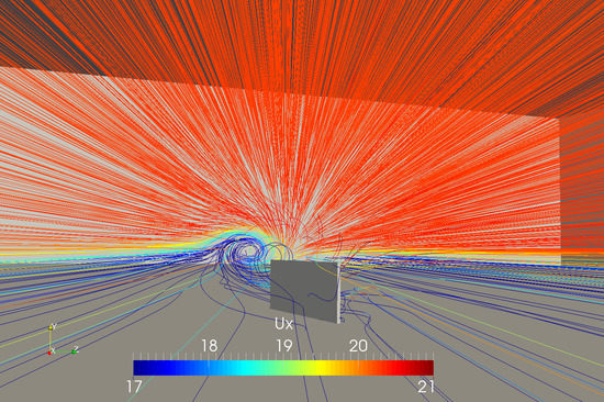
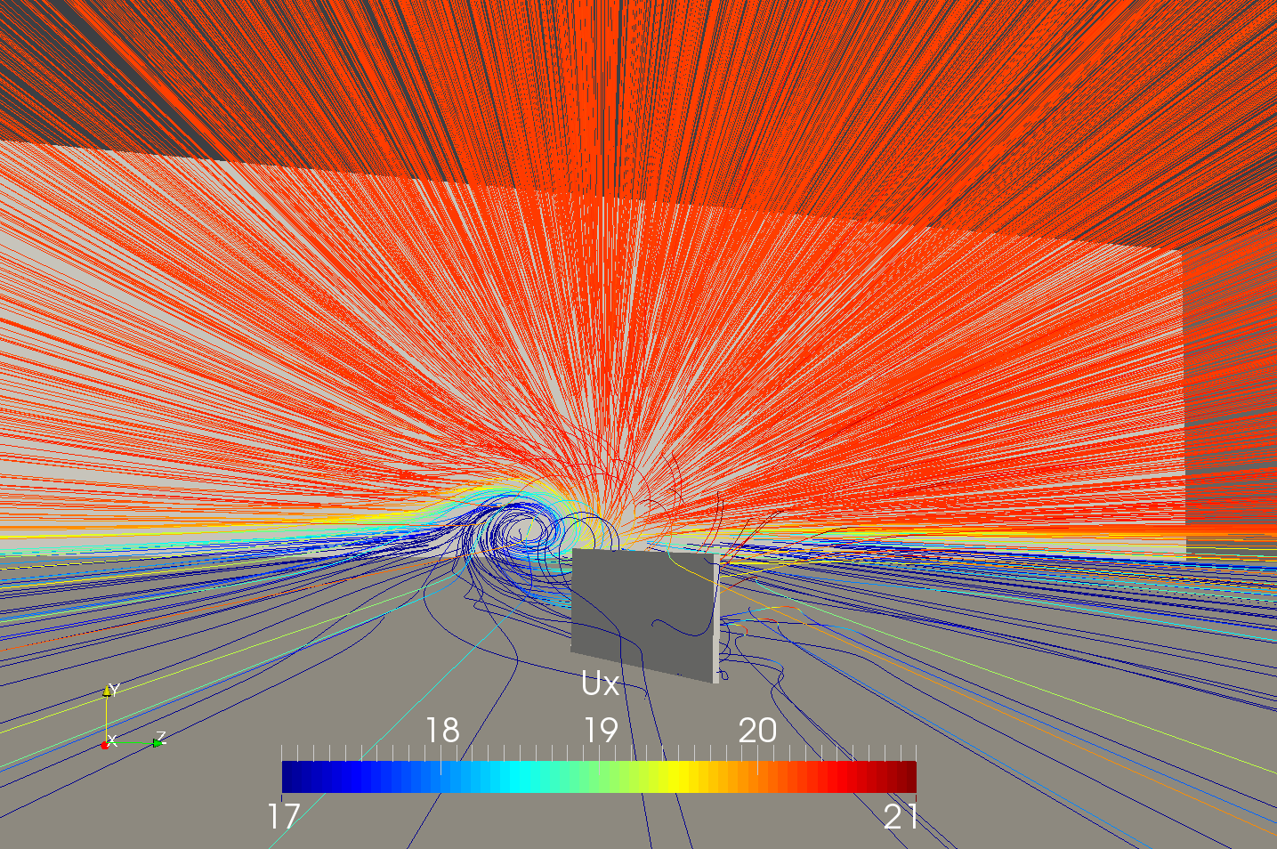
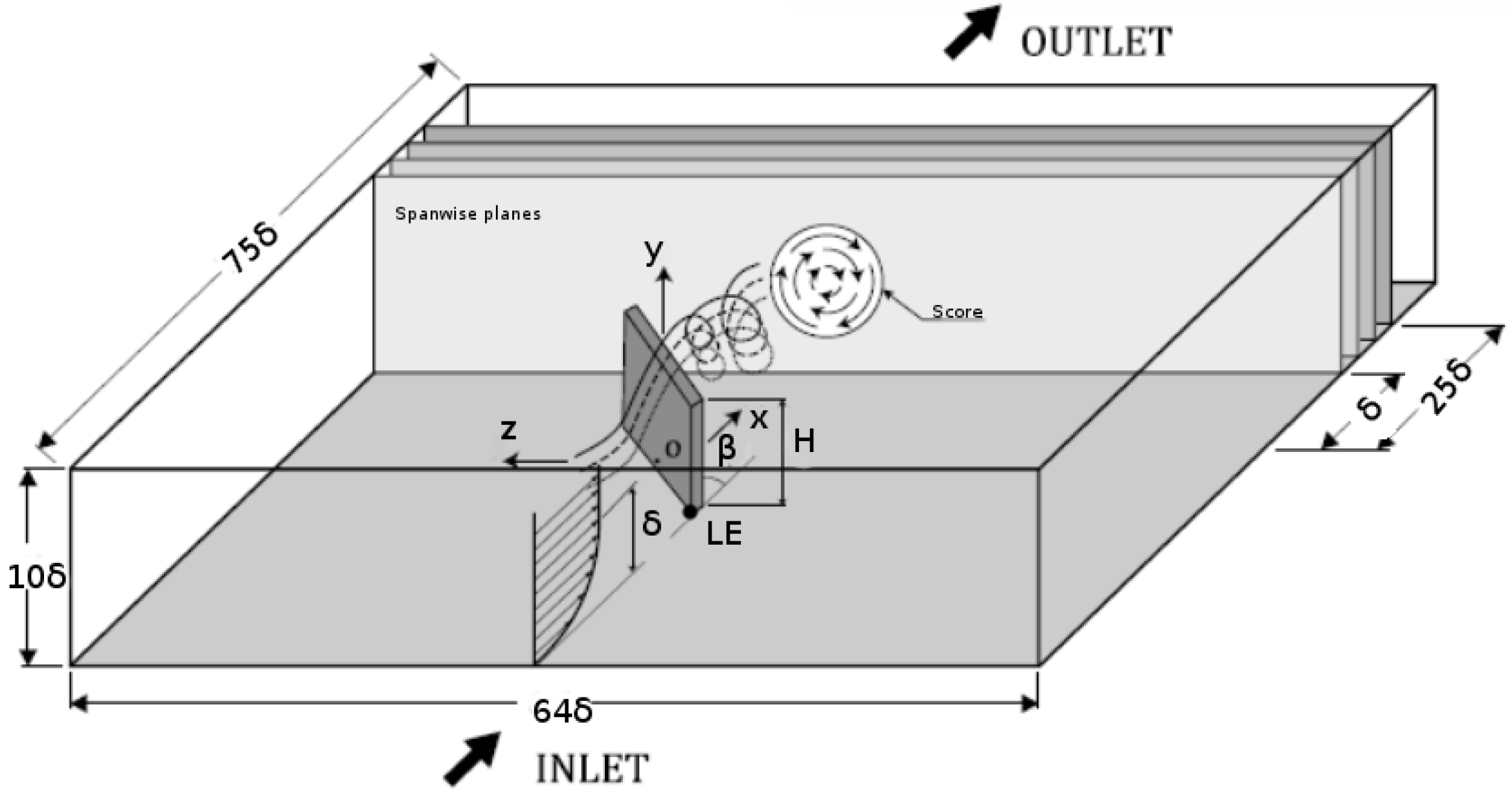
The computational setup consists of a flat plate with a single VG whose leading edge (LE) is placed at $10.25$ m from the inlet boundary, see Figure 1. This passive device consists of a rectangular vane with a length twice its height (H), which varies to make possible the parametric study. The normalization of the domain is done with respect to the conventional VG height (H); this height is equal to the boundary layer thickness $\delta =0.25$ m at the leading edge (LE) of the VG. Different boundary conditions have been set for the domain limits. According to Gutierrez-Amo et al. [23], the ceiling and the two lateral sides were set as slip conditions. Additionally, nonslip conditions were set for the vane and flat plate surfaces, while the upstream part of the domain was specified as inflow conditions with prescribed velocity according to the undisturbed velocity. The downstream part was set as an outlet assuming a fully developed flow.

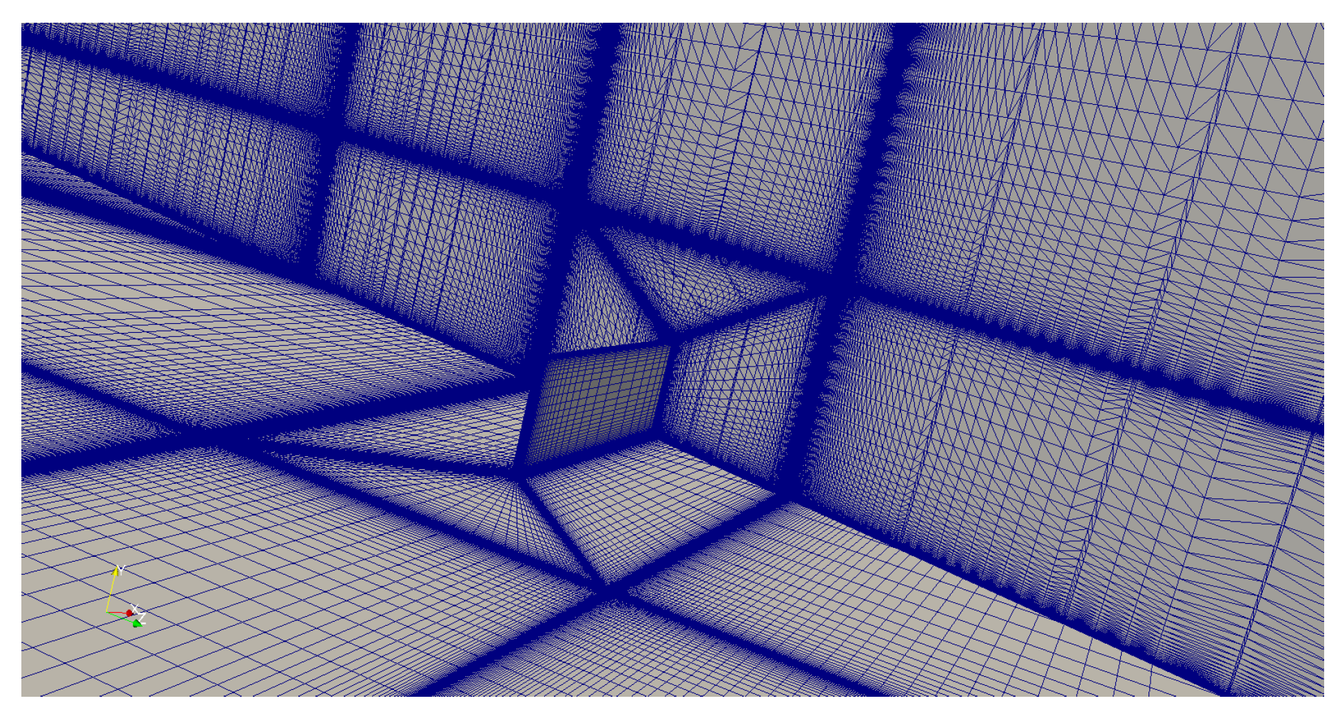
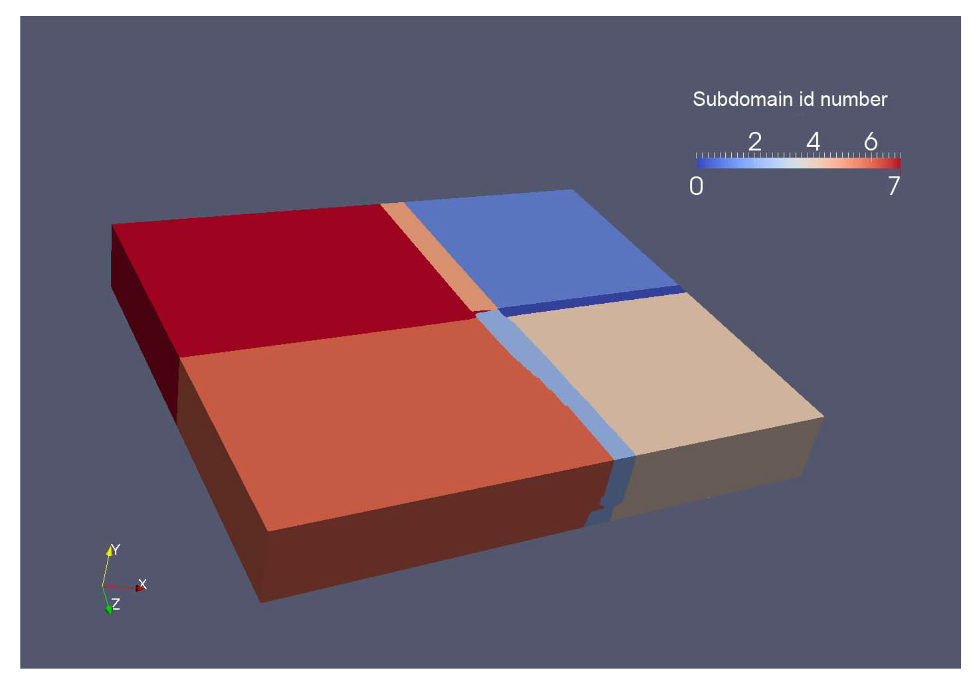
The strategy carried out to save computational cost was to divide the mesh in blocks because the cell density in the mesh is different in order to capture more accurate results in those places where the vortex is generated, around and downstream of the VG. Each block has a particular stretching factor in the three spatial coordinates, as shown in Figure 2.

Two types of structured meshes in the computational domain were designed according to the different VG heights used for the parametric study. A first mesh with around 12 million hexaedral cells and 64 blocks for the 0.2H and 0.4H VG height cases, and a second mesh sized 11 million hexaedral cells and 44 blocks for the other three VG height cases were used with a normalized height of the closest cell to the wall of $\frac{\Delta y}{\delta }=1.5\times {10}^{-6}$. Both meshes have a block-based structure and are divided in regions which allow a different grid resolution. The mesh generation was performed by an OpenFoam block-mesh utility that reads a dictionary where points, faces, cells, and boundary are defined. A similar meshing strategy as that in Urkiola et al. [17] was followed in order to achieve a high quality grid.

The computation domain was normalized with respect to the conventional VG height H, which it is equal to the local boundary layer thickness at the leading edge of the VG. Thus, its width is 64 times, its height 10 times, and its length 75 times the local BL thickness (Figure 1).

In the present study, four incident angles were analyzed, $\beta =10$${}^{\circ }$, 15${}^{\circ }$, 18${}^{\circ }$, and 20${}^{\circ }$ Six VG heights were considered, 0.2H, 0.4H, 0.6H, 0.8H, H and 1.2H; for every case, the VG length is 2H. The free stream velocity of the fluid is $U_{\infty }$ = 20 $\mathrm{m}·{\mathrm{s}}^{-1}$, the kinematic viscosity has a value of $\nu =1.85185\times {10}^{-4}$ m${}^2$s${}^{-1}$, and the Reynolds number Re = 27,000. The Reynolds number definition can be seen in Equation (1), where $U_{\infty }$ represents the free stream velocity, $\delta$ the boundary layer thickness where the VG leading edge is located, and $\nu$ the kinematic viscosity.

$$Re=\frac{U_{\infty }\delta }{\nu }$$

(1)

The domain was automatically decomposed in eight subdomains as shown in Figure 3 in order to solve in parallel with all the workstation cores available, making the solving process faster and more efficient. Simulations were performed on a personal server-clustered parallel workstation with Intel^® Xeon^® E5-2630 v3 CPU 2.40GHzx16 cores and 32 GB RAM on 64 bits Linux. The simulations were completed when the residuals of the velocity, pressure, and turbulence fields reached previously defined threshold values. A qualitative convergence was considered for residuals decay to ${10}^{-5}$ during the simulation. Taking into account the six VG heights and the four incident angles considered in this parametric study, twenty-four simulations were carried out. The average computational cost of each simulation took approximately 194 h.

All variables needed to estimate the vortex features were extracted from eleven spanwise planes placed downstream of the VG (Figure 1) in each simulation. The planes were normal to the main flow direction and located from 1 to 25 times the local boundary layer thickness $\delta$ downstream of the VG trailing edge (TE).

Mesh Quality Study

For all meshes used in this study, two different mesh quality parameters were studied, such as the mesh orthogonality and the skewness. The obtained values for these two parameters are shown in

Table 1. Quality meshing parameters for each analyzed vortex generators (VG) case.

VG Case	Non-Orthogonality (Max)	Non-Orthogonality (Avg.)	Max. Skewness (-)
$1.2\mathrm{H}$	66.58${}^{\circ }$	12.71${}^{\circ }$	2.87
H	65.32${}^{\circ }$	12.69${}^{\circ }$	3.33
$0.8\mathrm{H}$	64.85${}^{\circ }$	12.77${}^{\circ }$	3.22
$0.6\mathrm{H}$	66.66${}^{\circ }$	13.02${}^{\circ }$	2.92
$0.4\mathrm{H}$	63.28${}^{\circ }$	12.60${}^{\circ }$	3.56
$0.2\mathrm{H}$	60.07${}^{\circ }$	12.60${}^{\circ }$	3.56

for the six VG meshes.

The non-orthogonality (nO) measures the angle between a line that connects the center of two adjacent cells and the normality of their common face; any non-orthogonality value satisfying the condition of $nO<70$ is a safe value and for all the VG cases, the used meshes nO values lie in this safe zone. The skewness represents the distance between the point where the common face of two cells is crossed by the line that connects the center of those two cells and the center of this common face. The smaller the value for skewness, the better, and any value bigger than 20 may suggest lack of accuracy. Both meshing parameters, non-orthogonality and skewness, are in the range explained ahead for all meshes.

3. Results

According to Martinez-Filgueira et al. [32], the vortex center path, vortex size, and peak vorticity of the vortex are the most interesting parameters to show the characteristics of the progress of the streamwise vortexes generated downstream in rectangular VGs. Yao et al. [33] proposed the point with the highest peak streamwise vorticity as the center of the vortex core. The peak vorticity is the point which has the largest vorticity of the vortex in a spanwise plane past the trailing edge of the VG and normal to the streamwise direction. Thus, the vortex trajectory can be obtained looking at the evolution of the vortex center in the different spanwise planes downstream of the VG. The primary vortex lateral and vertical path produced by VGs have a key role in the momentum mixing performance.

3.1. Vortex Path

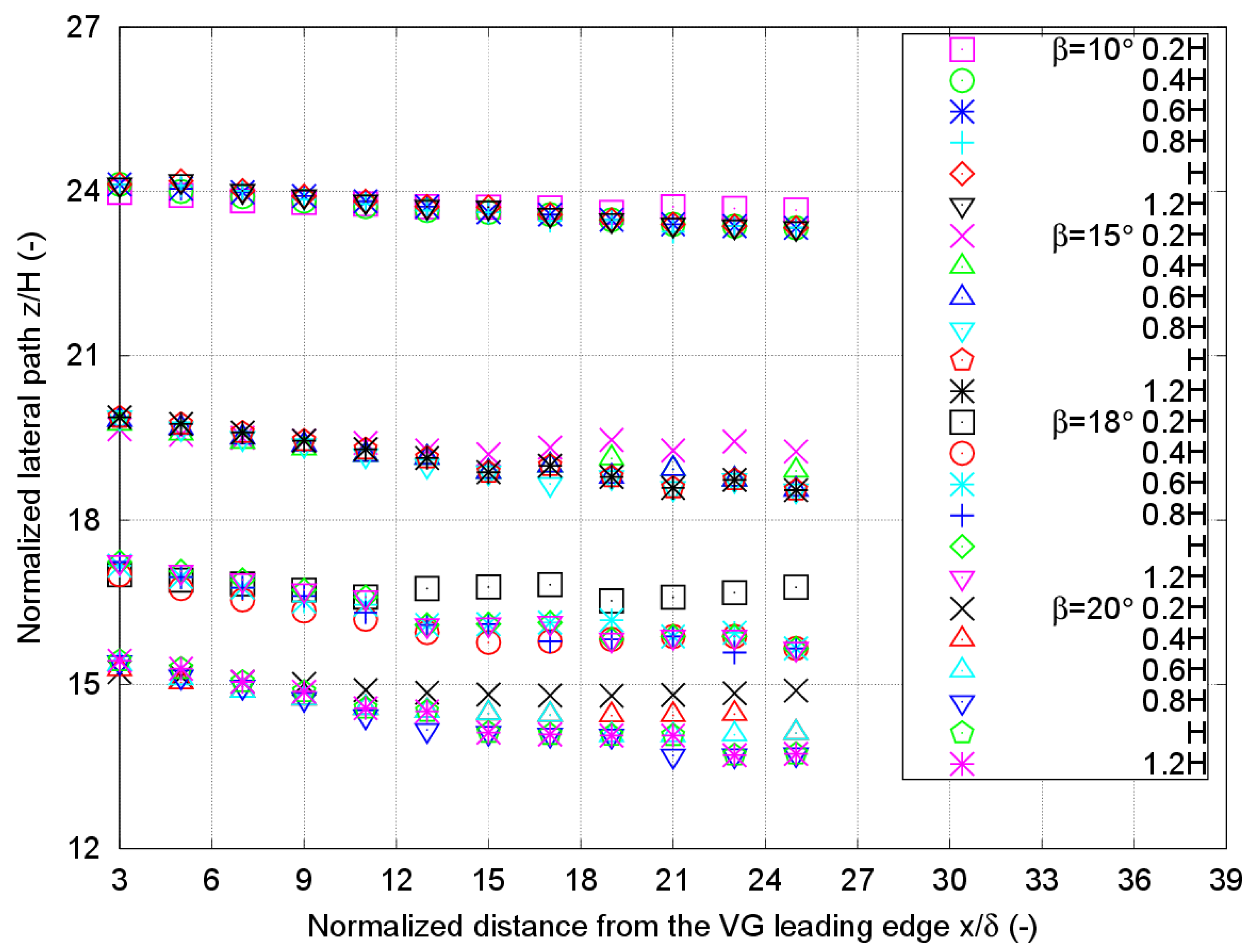
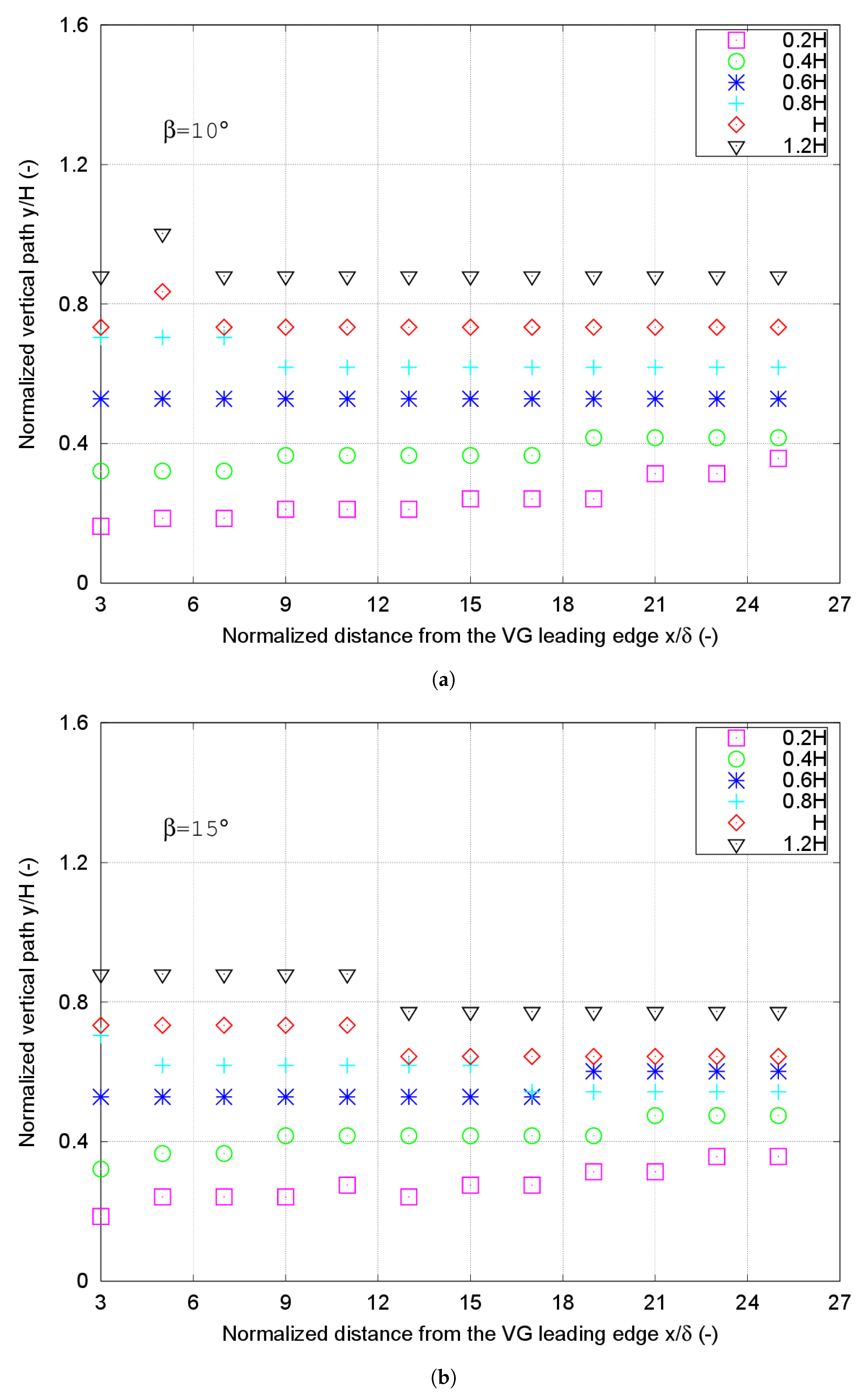
Vertical y and lateral z coordinates of the vortex center were calculated in spanwise planes to the streamwise direction placed at different distances x downstream of the VG. With these calculations, the vortex center deviation can be obtained for each simulated case corresponding to the six different heights.

Figure 4 and Figure 5 show the lateral and vertical paths for the four different incident angles and the six different VG heights, respectively.

As shown in Figure 4, a lateral evolution of the vortex center can be observed; this movement evolves along the distance x from the VG trailing edge at the considered different spanwise planes and for all the simulations. This lateral evolution shows a deviation of the vortex center in the direction indicated by the VG trailing edge. The nondimensional vortex center lateral paths observed in the figure follow a similar trend for the incident angles $\beta =$ 15${}^{\circ }$, 18${}^{\circ }$, and 20${}^{\circ }$, having higher lateral deviation for the highest VG height, 1.2H.

When looking at the 0.2H and 0.4H VG height cases, the deviations observed are smaller than the deviations corresponding to higher VGs. When analyzing the $\beta$ = 10${}^{\circ }$ incident angle, the deviation observed is also smaller than the deviation corresponding to bigger incident angles.

Regarding the vertical path shown in Figure 5, the vortex centers calculated just past the VG trailing edge initially have a vertical position which is similar to the VG height for all the VG cases. As observed in the four plots corresponding to the four incident angles in Figure 5, there is not a meaningful vertical deviation. For the 0.8H, H, and 1.2H height cases, a relatively small downward deviation can be appreciated. On the other hand, for the two smallest height cases, the vertical path is pointing upwards. The reason for this upward deviation can be found in the fact that the lower VG vanes are within the inner part of the local boundary layer and, consequently, the viscous shear could prevail and have a determining influence when interacting with the wall.

The cases with similar VG height to the local boundary layer thickness follow the conclusions of Fernandez-Gamiz et al. [24], who concluded that there is probably no vertical deviation of the vortex center position lengthwise in the streamwise direction.

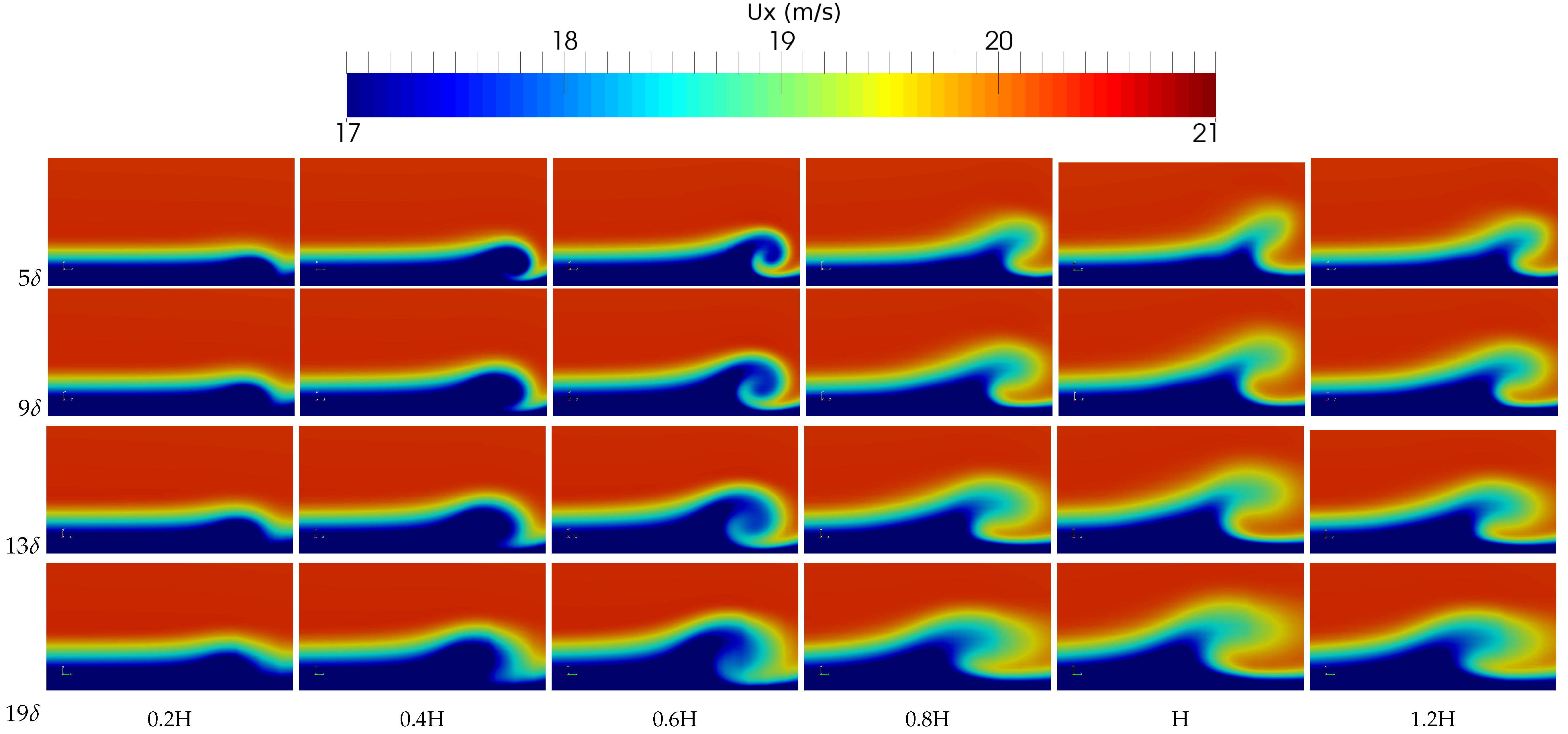
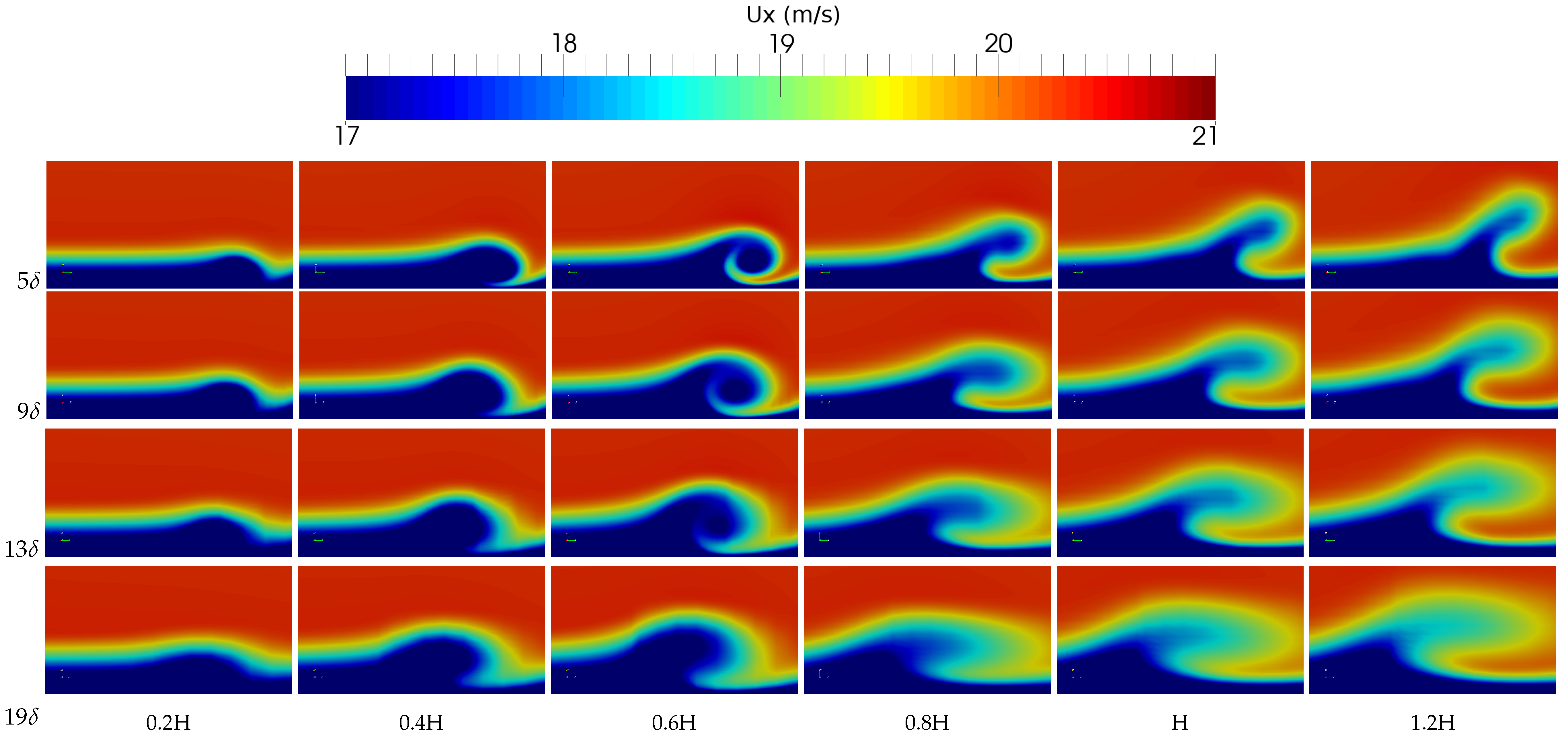
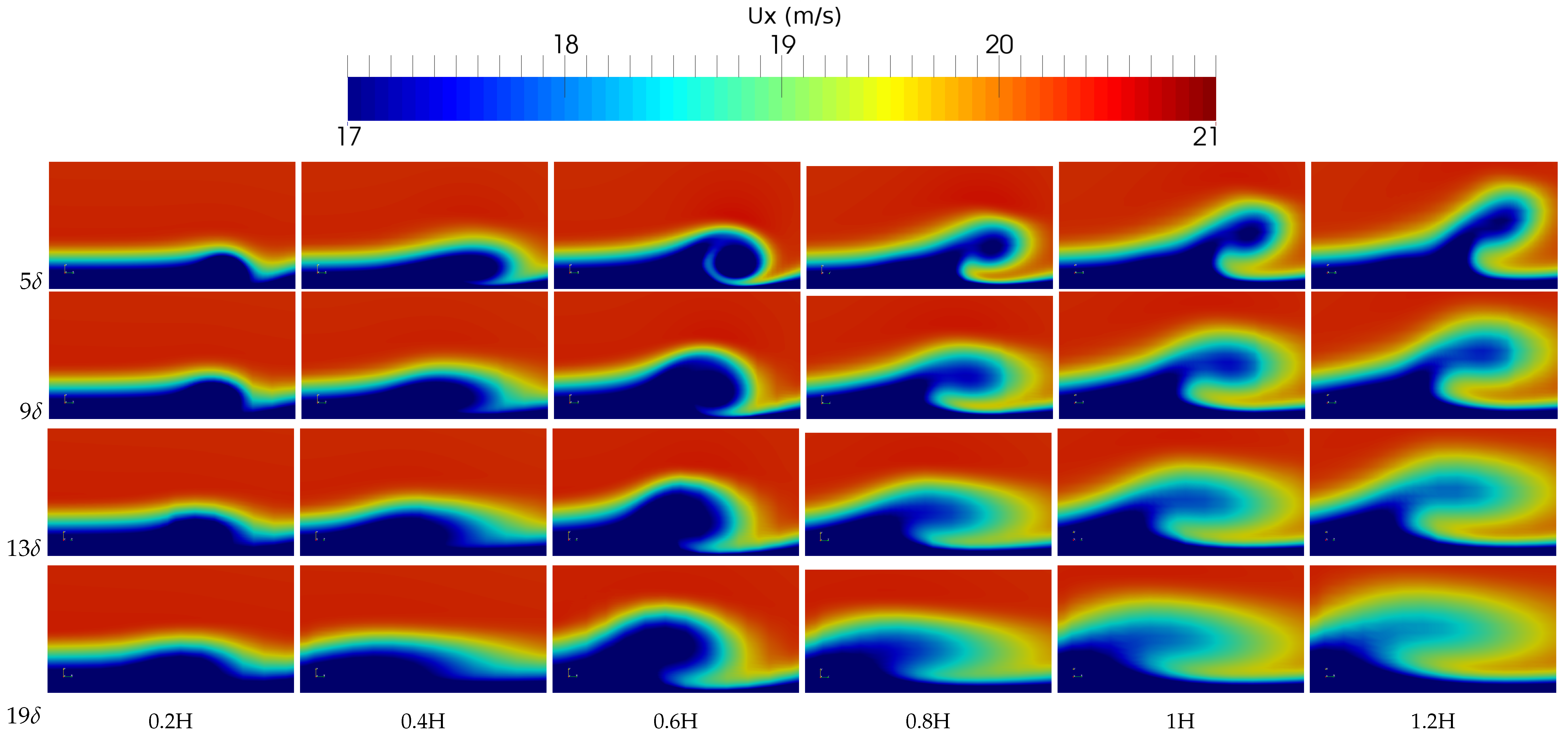
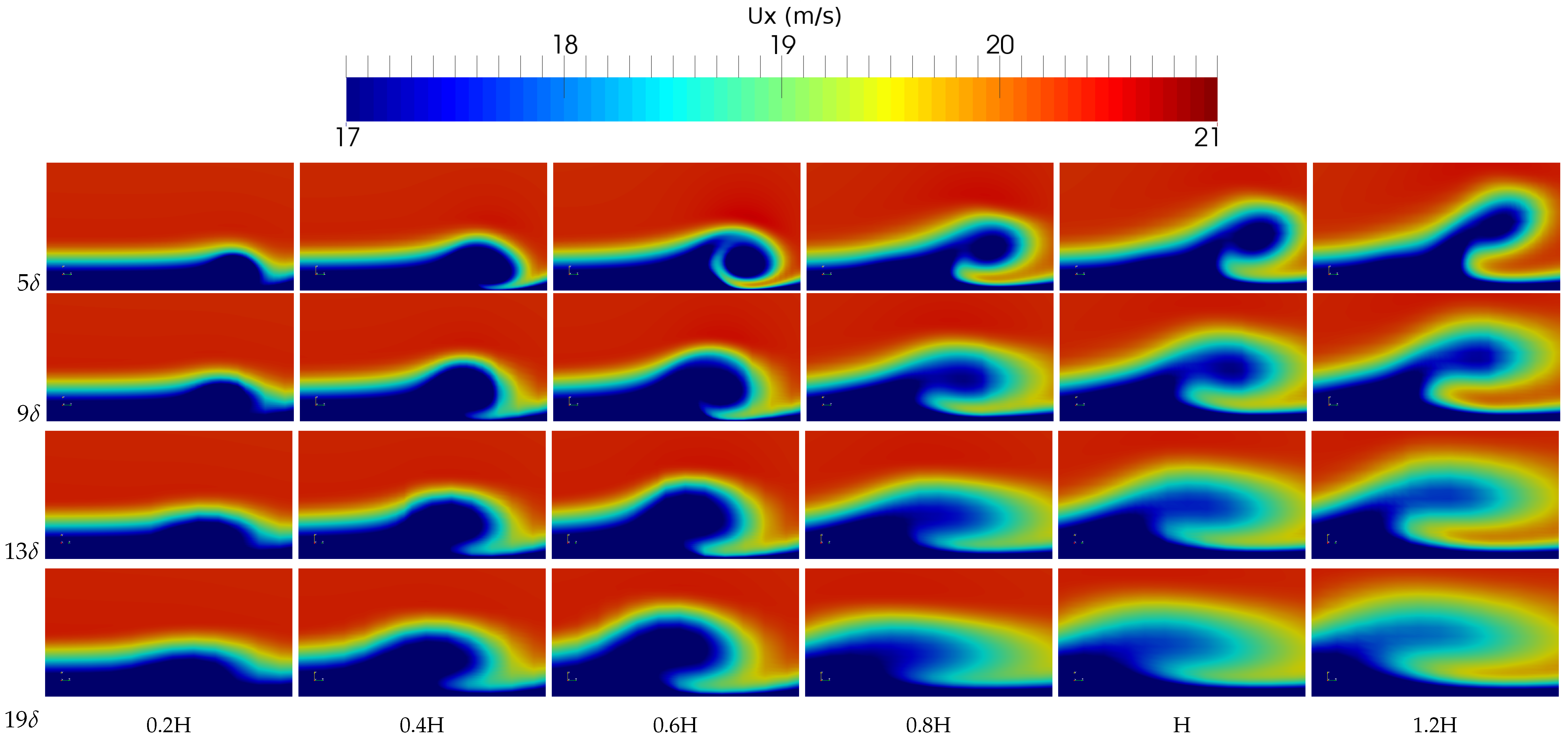
In the four figures of Appendix A, Figure A1, Figure A2, Figure A3 and Figure A4, the primary vortex evolution can be observed. These four figures depict the axial velocity distribution U${}_x$ at four different planes normal to the streamwise direction and located at distances proportional to the local boundary layer thickness $\delta$ for the six VG height and four incident angles.

The formation and evolution of the primary vortex is clear for all the simulations and even more evident in the 0.6H VG height case. Furthermore, the vortex size increases as the planes are farther away from the VG trailing edge. This size increase indicates a lower gradient of velocities from the vortex center to the outer part of the vortex. It can be qualitatively observed in the four figures of Appendix A that vortexes of increasing size are obtained for bigger incident angles $\beta$ and higher VGs.

The lateral deviation of the vortex path can be also observed in the figures as the distance from the vortex generators’ TE increases. This displacement in the z-axis occurs towards the side where the VG is rotated and is depicted for all the VG cases and is more evident for the highest incident angles $\beta$ = 18${}^{\circ }$ and 20${}^{\circ }$.

Summarizing the qualitative analysis made by means of the four figures shown in the Appendix A, the primary vortex can be clearly identified; it is simulated and captured relatively well with the exception of the smallest VG height case. where the vortex is hardly appreciated, perhaps because of its position near to the inner part of the local boundary layer.

3.2. Vortex Size

The vorticity on a perpendicular plane to the streamwise direction is a function of three variables, the distance from the vortex center, the peak vorticity of that plane, and the radius size.

The calculation of the vortex radius is a difficult task for experimental and CFD data. Martinez-Filgueira et al. [32] and Fernandez-Gamiz et al. [25] showed that the vorticity profile generated by a vortex generator in a plane normal to the streamwise direction and in a line passing horizontally through the vortex center has a Gaussian distribution-type shape and that the vortex center defined by the peak vorticity is located in the center of this Gaussian distribution.

The vorticity profile fits the Gaussian distribution better in the peak values than in the tails. A way to overcome this fitting problem in the tails comes by a innovative definition of the vortex size by means of the concept of the half-life radius ($R_{05}$). The $R_{05}$ is defined as the radial distance from the vortex center to the point where the half-value of the peak vorticity is located, as proposed by Bray [34].

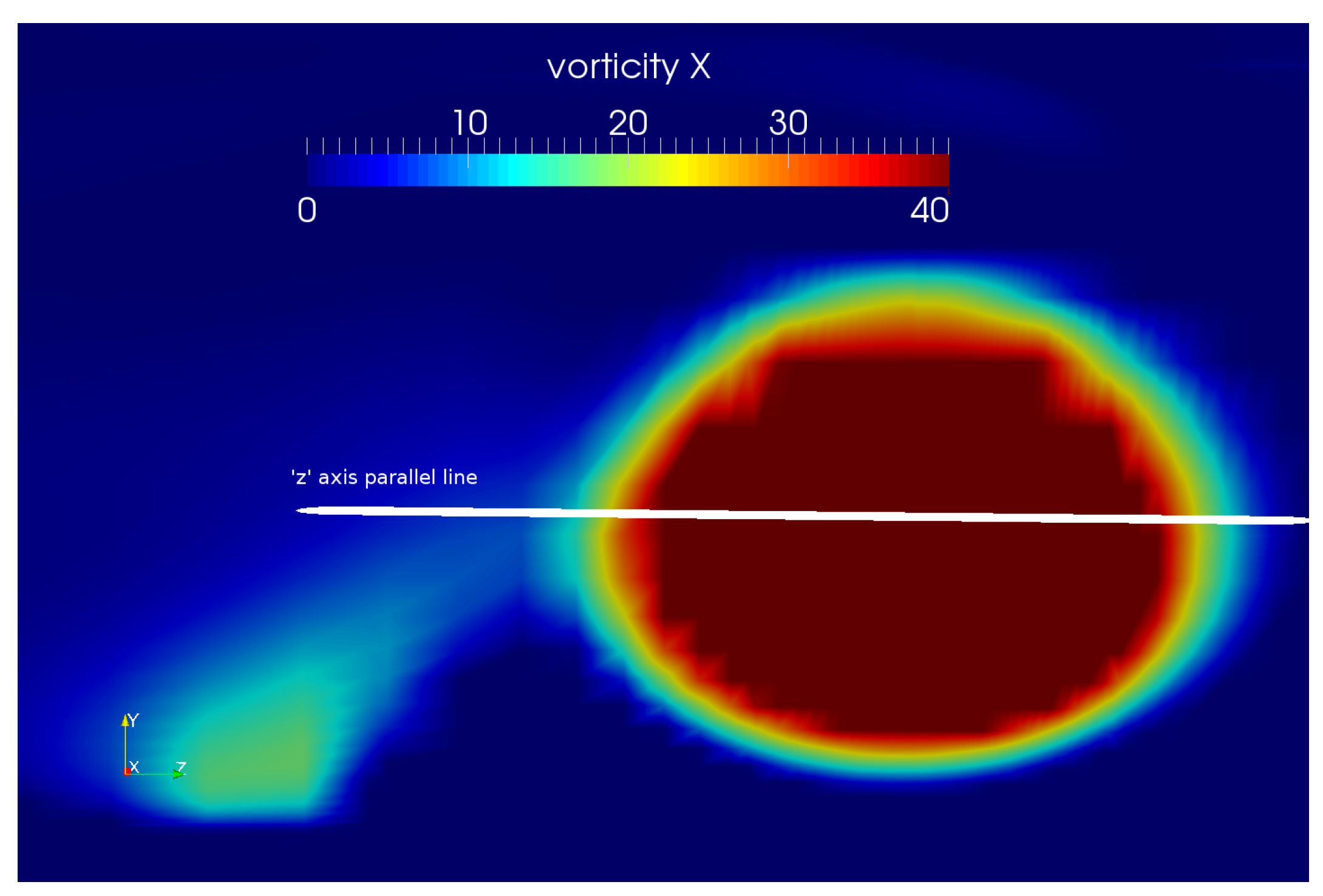
In Figure 6, the vorticity distribution in a spanwise plane normal to the free stream velocity at x distance from the VG trailing edge can be observed. In order to obtain the vorticity profile associated to the vortex center, the vorticity values of a horizontal line (shown in white color) passing through the vortex center are extracted. For each VG case, the vorticity profile that crosses the vortex center of 12 spanwise planes normal to the streamwise direction was extracted. These planes are placed from 3$\delta$ to 25$\delta$ distances from the trailing edge of the VG.

Equations (2) and (3) represent the Gaussian distribution of the vorticity in a plane normal to the streamwise velocity, where r represents the radial coordinate, $\omega$ is the vorticity expressed in s${}^{-1}$, $R_{0.5}$ the half-life radius in m and the dimensionless constant k with value of 1. According to Martinez-Filgueira et al. [32], the $R_{0.5}$ can be determined by calculating the half-value of the peak voticity ${\omega }_{peak}$.

$$\omega \left(r\right)={\omega }_{peak}{e}^{k{\left(\frac{r}{R_{0.5}}\right)}^2}$$

(2)

$$\mathrm{if}r=R_{0.5}\mathrm{and}\omega \left(r\right)=0.5\left\{\begin{array}{c}k=ln\left(\frac{\omega \left(R_{0.5}\right)}{{\omega }_r}\right)=ln\left(\frac{1}{2}\right)\hfill \\ \omega \left(r\right)={\omega }_{peak}{e}^{ln\left(\frac{1}{2}\right){\left(\frac{r}{R_{0.5}}\right)}^2}\hfill \end{array}\right.$$

(3)

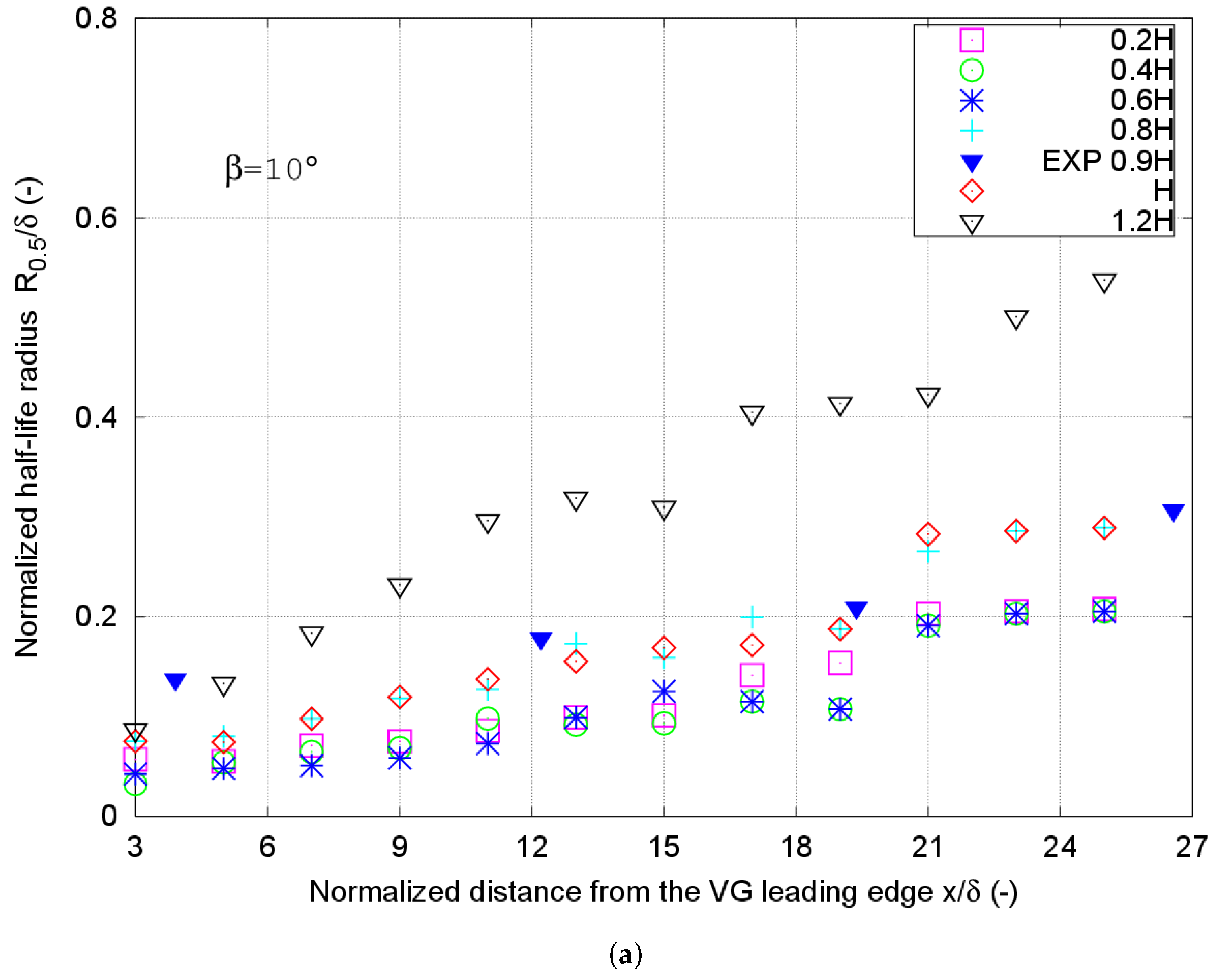
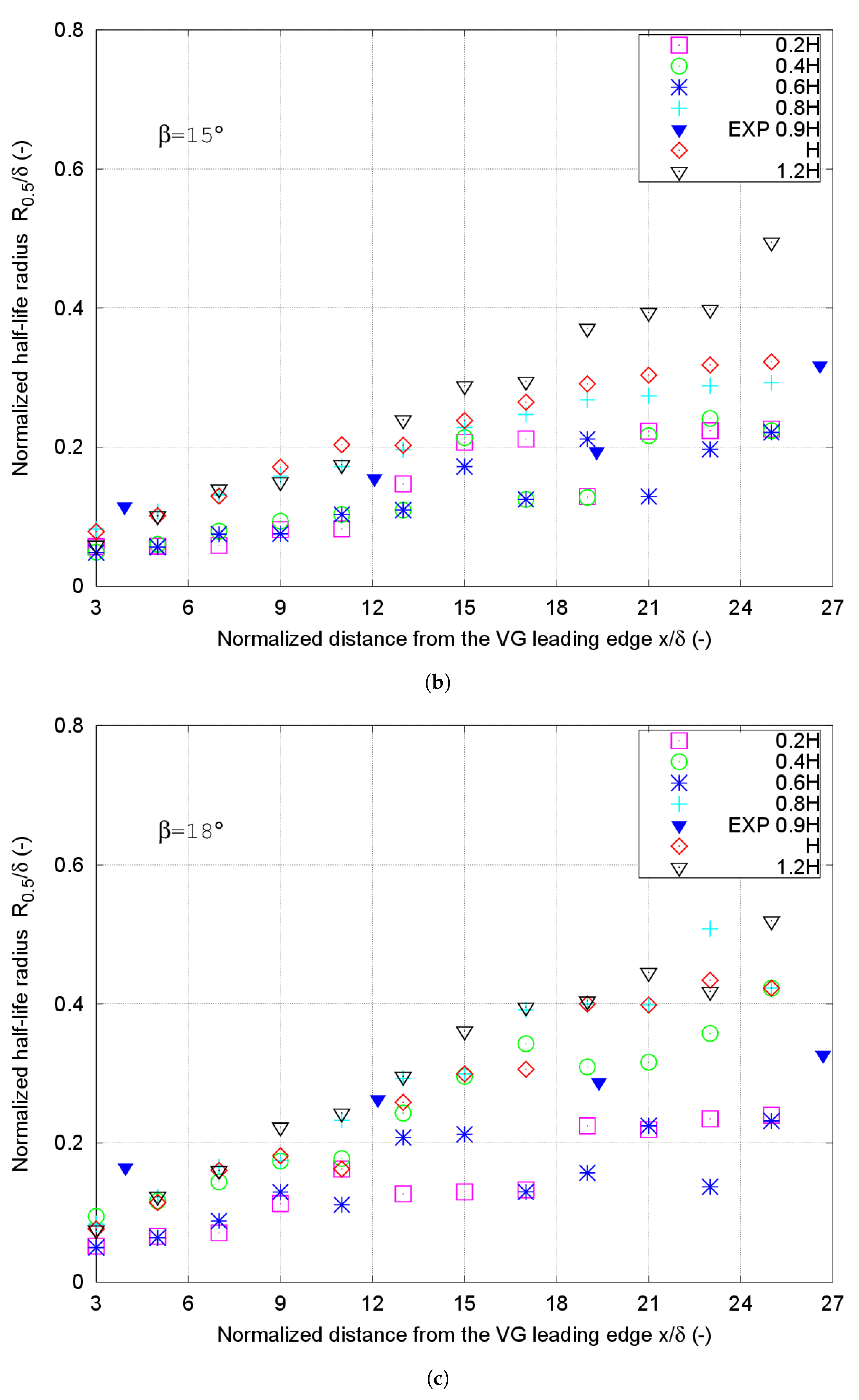
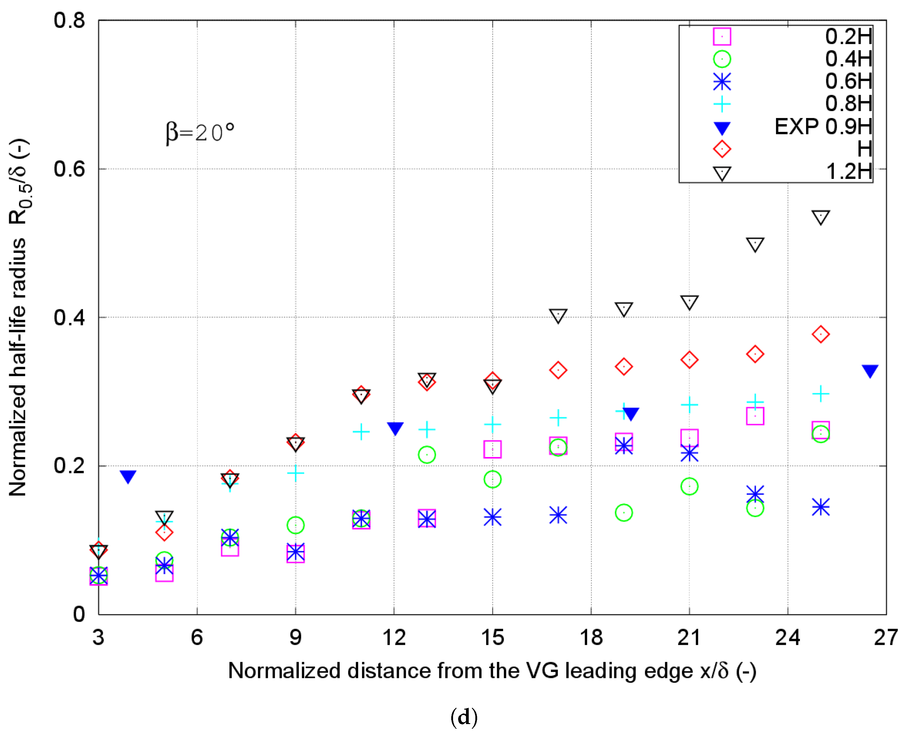
Figure 7 shows the CFD results for the $R_{0.5}$ considering the four different incident angles, $\beta$ = 10${}^{\circ }$, 15${}^{\circ }$, 18${}^{\circ }$, and 20${}^{\circ }$, and some of the experimental (EXP) measurements obtained by Bray [34]. Represented values are normalized with respect to the local boundary layer thickness ($\delta$) in the VG leading edge.

The vortex size considering the criteria of the $R_{0.5}$ shows an increasing trend along the planes placed normal to the streamwise direction. This increasing trend obtained in the CFD simulations is as well observed in the measurements of Bray [34] for the incident angles. As it gets farther from the vortex generator TE, the half-life radius gets higher values. Although the slope representing the evolution of the vortex size increases as the incident angle does, it is more dependent on the distance from the trailing edge of the VG.

Considering the VG height, bigger values of half-life radius are obtained for higher VG vanes. Even if the highest vane follows a similar trend, with each incident angle, it takes bigger values in small distances from the TE for the 10${}^{\circ }$ incident angle. The 10${}^{\circ }$ incident angle also shows a bigger difference between the half-life radius values of the highest VG case than other incident angles.

A qualitative study of the vortex size can also be done in Figure A1, Figure A2, Figure A3 and Figure A4 of the Appendix A. The velocity fields show for every VG case the vortex formation for several spanwise planes downstream of the vane and for a different incident angle in each figure. The interaction with the surface is clearly bigger for 0.2H and 0.4H VG heights, but also in these both cases, an evolution is identified where the vortex size seems bigger as the plane is further from the VG. The vortex formation gets more obvious for $\beta =18$${}^{\circ }$ and $\beta =20$${}^{\circ }$. Vortexes are also generated, as expected, at a bigger height as the VGs are higher. Therefore, quantitative and qualitative results show the same conclusions about the development of the vortex size.

Thus, the main vortex characteristics of this complex 3-D flow were captured and described in spite of the viscous interactions between the fluid and secondary structures and the wall. The evaluation of the CFD techniques performance of the characterization of this type of flows is important, since these flows are the most broadly used in order to solve this kind of problem.

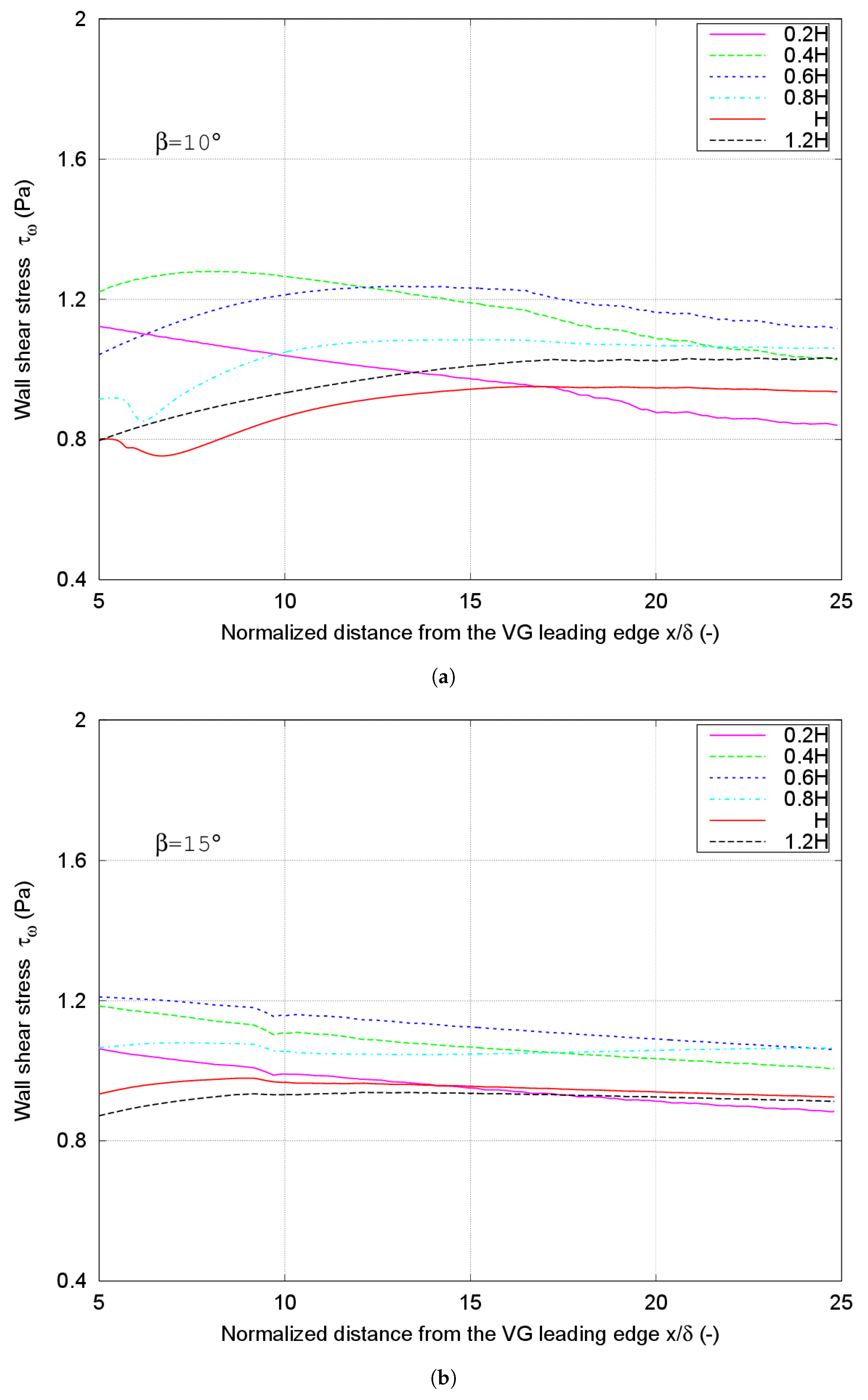
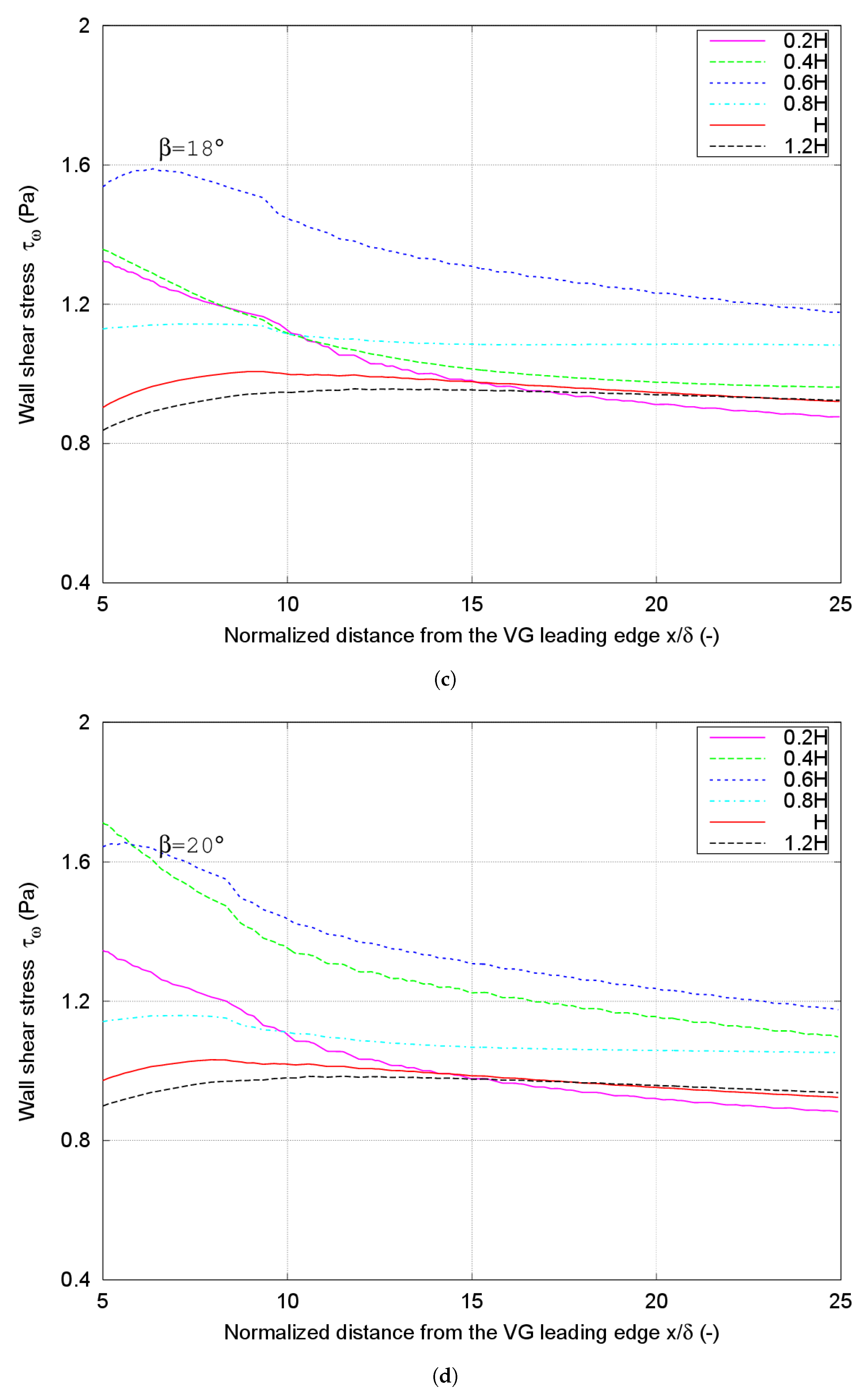
3.3. Wall Shear Stress

The wall shear stress ${\tau }_{\omega }$ is a significant parameter for the understanding of the flow separation. According to Godard et al. [35], higher values of wall shear stress are directly related with the delay or avoidance of the separation of the flow.

The wall shear stress of all VG height cases and four incident angles, $\beta$ = 10${}^{\circ }$, 15${}^{\circ }$, 18${}^{\circ }$, and 20${}^{\circ }$, was calculated. For higher values of the shear stress, the boundary layer gets better attached to the surface. In Figure 8, the wall shear stress ${\tau }_{\omega }$ is shown for four incident angles depending on the distance from the TE of the VG.

The wall shear stress shows the highest value for the 0.6H VG height case for all the incident angles. For the incident angle $\beta$ = 10${}^{\circ }$, the 0.4H VG height case starts with a big value and decreases as the cutting planes are farther from the VG trailing edge. The wall shear stress varies with the vane heights and the different incident angles. This variation is even more obvious for incident angles of $\beta$ = 18${}^{\circ }$ and $\beta$ = 20${}^{\circ }$, where higher values of wall shear stress are observed for the 0.4H and mainly the 0.6H VG height cases, and as long as the downstream distance from the TE is bigger, the wall shear stress curve decreases. However, for the 0.8H, H, and 1.2H VG height cases, the wall shear stress is almost constant for the four incident angles and all along the streamwise direction, with a small variation for the incident angle $\beta$ = 10${}^{\circ }$.

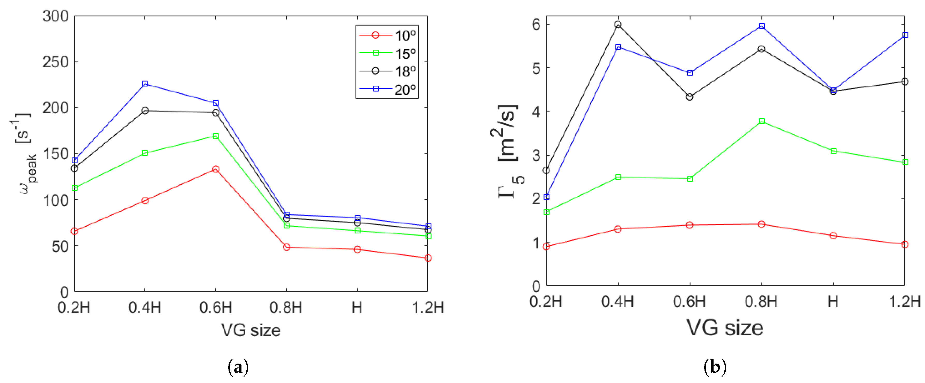
3.4. Vortex Strength

As commented on at the beginning of Section 3, the vortex peak vorticity is one of the main characteristics of a vortex, so the maximum value of the streamwise vorticity was studied for cases and incident angles at a plane placed to $5\delta$ distance from the TE of the VG, see Figure 9a. Additionally, the strength of the vortex was evaluated in the present study by the circulation $\left({\Gamma }_5\right)$ defined by Equation (4), see Yao et al. [33]. It was calculated by finding the peak vorticity over the area surrounding the vortex core in cross-flow plane positions normal to the wall and at the distance of $5\delta$ downstream of the VG trailing edge. Figure 9b presents the values of the circulation against the device heights.

$${\Gamma }_5=\frac{{\omega }_{peak}·\pi ·R_{0.5}}{0.693}$$

(4)

The circulation measured at $5\delta$ roughly varies for cases where device heights are larger than 0.4H. Furthermore, the highest values are obtained for $\beta$ = 18${}^{\circ }$ and $\beta$ = 20${}^{\circ }$ incident angle cases, following a similar trend in these two incident angles. In agreement with the values obtained for wall shear stress in Figure 8c,d, where the highest values are for $\beta$ = 18${}^{\circ }$ and $\beta$ = 20${}^{\circ }$ and 0.4H and 0.6H VG heights, Figure 9b shows that the highest circulation values are reached mostly for the same incident angles and heights. Regarding this issue, 0.4H and 0.6H VG heights and $\beta$ = 18${}^{\circ }$ and $\beta$ = 20${}^{\circ }$ incident angles show the best performance in terms of vortex strength and generation of wall shear stress.

4. Conclusions

In the present study, the primary vortex generated by a single vane-type vortex generator (VG) has been characterized. Numerical simulations were carried out using open-source OpenFOAM code for four incident angles, $\beta$ = 10${}^{\circ }$, 15${}^{\circ }$, 18${}^{\circ }$, and 20${}^{\circ }$ and six VG heights, 0.2H, 0.4H, 0.6H, 0.8H, H, and 1.2H, where H is the value of the BL thickness $\delta$ at the VG position. The vortexes generated by these VGs were simulated considering turbulent, steady, state and incompressible flow with a Reynolds number of $Re$ = 27,000 based on the local BL thickness $\delta$ at the VG position.

The parameter used to measure the vortex size was the half-life radius $R_{0.5}$, and the results showed that this value is significantly dependent on the VG height and vane incident angle. In general, the higher the VG height, the larger the size of the primary vortex. For the lowest incident angle $\beta$ = 10${}^{\circ }$ studied, the largest size of the vortex is achieved by the highest VG case of 1.2H. However, as the incident angle increases, the differences in the size of the vortex in comparison with smaller vanes are not relevant.

As expected, the vortex trajectory is affected by the VG height, as well as by the incident angle $\beta$, and this path variation is more evident for the larger angles. In each simulated case, the vertical trajectory of the vortex is almost constant, with the exception of the 0.2H VG height case. This behavior may be due to the low VG height, which is within viscous sublayer where viscous effects are dominant and, therefore, an interaction with the wall appears.

Regarding the wall shear stress, two conclusions can be drawn. Firstly, a variation of the wall shear stress with the incident angle was confirmed. Larger wall shear stress values were obtained for higher incident angles $\beta$ = 18${}^{\circ }$ and 20${}^{\circ }$, and these values decrease along the streamwise direction. Secondly, the VG sizes 0.4H and 0.6H at the incident angle of $\beta$ = 20${}^{\circ }$ reached the largest wall shear stress along the streamwise direction. Additionally, the circulation shows the highest values are for 0.4H and 0.6H VG heights and $\beta$ = 18${}^{\circ }$ and 20${}^{\circ }$ at $5\delta$ distance from the TE, results that agree with the obtained wall shear stress conclusions. Therefore, those vane heights and incident angles seem to be the best option for flow separation control.

CFD techniques are the most commonly methods used to improve the optimization of VGs on wind turbine blades, so the results and information presented by this study can be used as a model and guidance for effective implementation of VGs. Due to the high variety of parameters that have influence in the problem, such as VG height and orientation, a precise understanding of the flow gains importance for successful application of VGs. A further step would be the simulation of different VG sizes and orientation in typically used airfoils for wind turbine blades at different Reynolds numbers.