Numerical Analysis of Flow in Building Arrangement: Computational Domain Discretization
by
 , , , and
Marcin Sosnowski
1 ,
,
Renata Gnatowska
2,*,
Karolina Grabowska
1,
Jarosław Krzywański
1 and
Arkadiusz Jamrozik
2 1
Faculty of Mathematics & Natural Sciences, Institute of Technology & Safety Systems, Jan Dlugosz University in Czestochowa, Armii Krajowej 13/15, 42-200 Częstochowa, Poland
2
Faculty of Mechanical Engineering and Computer Science, Institute of Thermal Machinery, Częstochowa University of Technology, Armii Krajowej 21, 42-200 Częstochowa, Poland
*
Author to whom correspondence should be addressed.
Appl. Sci. 2019, 9(5), 941; https://doi.org/10.3390/app9050941
Submission received: 23 December 2018
/
Revised: 10 February 2019
/
Accepted: 28 February 2019
/
Published: 6 March 2019
(This article belongs to the Section Environmental Sciences)
Abstract
:The progress in environmental investigations such as the analysis of building arrangements in an urban environment could not have been expanded without the use of computational fluid dynamics (CFD) as a research tool. The rapid development of numerical models results in improved correlations to results obtained with real data. Unfortunately, the computational domain discretization is a crucial step in CFD analysis which significantly influences the accuracy of the generated results. Hence an innovative approach to computational domain discretization using polyhedral elements is proposed. The results are compared to commonly applied tetrahedral and hexahedral elements as well as experimental results of particle image velocimetry (PIV). The performed research proves that the proposed method is promising as it allows for the reduction of both the numerical diffusion of the mesh as well as the time cost of preparing the model for calculation. In consequence, the presented approach allows for better results in less time.
1. Introduction
1.1. Building Arrangements Analysis
The atmospheric boundary layer (ABL) is characterized by particular sensitivity to the type of terrain topography, as well as building geometry and arrangement. The ABL significantly contributes to climate and wind comfort, which is not only pedestrian comfort but also an issue of health risks resulting from dispersion of pollution. That is why the analysis of building arrangement has recently become an important issue in urban planning. The most widespread wind comfort criterion is based on mean wind velocity. However, the definition of comfort criterion should include turbulence due to mutual interactions of buildings in built-up areas. The generation of eddies in the wake behind buildings lead to an increase of flow instability. These eddies contain large and small scale turbulent structures and the resulting separation and recirculation zone is accompanied by areas of velocity fluctuations.
Other attempts in the development of more advanced wind comfort criteria were done by [1,2]. This research was directed towards the evaluation of periodic phenomena impact in external flow patterns on the flow structures in the vicinity of buildings. The results clearly indicate that the estimation of wind comfort based only on mean velocity is ineffective in the case of urban areas due to the increase of flow turbulence intensity caused by surface impact and aerodynamics of object interactions [3,4].
In numerical and experimental studies of urban area aerodynamics, the real build-up area is usually represented by simplified models in order to explain the analysed phenomena. A single building is usually simulated by a cuboid but it does not give a comprehensive assessment of the wind environment in built-up areas, where collective wind effects generated by adjacent buildings is very important [5,6,7]. In this case, the flow structure is determined by the geometry of building placement that is, the distance between objects or the relative proportions of their height. The mutual interaction of buildings in build-up areas leads to an increase of flow variability where the strong effect of periodicity results from the generation of eddies in the wakes behind the objects (large-scale and small-scale turbulent structures). Moreover, separation and recirculation zones are accompanied by areas of strong velocity fluctuations. In most cases, the studies of aerodynamic interactions in built-up areas are performed for few (usually two) cuboids [6,7,8,9].
The knowledge concerning the influence of building arrangement in the flow field on wind comfort relied mostly on experimental studies but in recent years researchers have focused on utilizing the capabilities of numerical methods in this field. Along with the rapid development of high-performance computers, Computational Fluid Dynamics (CFD) turned out to be one of the most promising tools in such research and as such, plays an important role in the environmental analysis [5,10,11,12,13,14].
CFD generates detailed information about flow parameters in entire numerical domains under precisely controlled conditions. Precision and credibility of CFD depend however on many factors, such as proper selection of boundary conditions and mesh generation, selection of numerical models and interpretations of the results. It is necessary to meet a number of requirements in order to carry out numerical modelling of wind impact on buildings. Flow calculations around buildings require knowledge of ABL characteristics where not only data concerning mean wind velocity is important but also turbulence levels and large-scale wind gusts data is required. However, meteorological data for an urban area, in most cases, does not give sufficient detail required as input data to CFD. This lack of data directly causes difficulties in the formulation of proper boundary conditions and this requires a careful fit of the turbulence model parameters and roughness conditions in a given boundary layer. Additionally, the flow and pressure fields are dominated by large-scale motions generated by ground objects. Selection of an appropriate method of numerical solution concerns, first of all, the choice of methodology for numerical analysis. The most obvious choices are the steady Reynolds-Averaged Navier Stokes (RANS) or unsteady RANS (uRANS) which are used most often since Large Eddy Simulation (LES) or hybrid URANS/LES techniques require much more computational time [15].
Apart from the selection and parameterization of a turbulence model, the discretization of the computational domain is a particularly important task in the case of flow modelling in built-up areas because it influences the CPU time, as well as the accuracy of the results [16,17,18]. Therefore an innovative approach to discretization method of the analysed domain representing the array of two buildings located in an urban environment is addressed in the carried out research.
1.2. Computational Domain Discretization
Advances in aerospace, power engineering [19,20], automotive [21,22], civil engineering [6,23,24], medicine [25,26] and other numerous branches of the industry could not have been achieved without the application of computational methods as a research tool. The primary and critical activity in numerical modelling is the computational domain discretization. It consists of dividing the analysed geometry into numerous small control volumes (elements).
1.2.1. Hexahedral Mesh
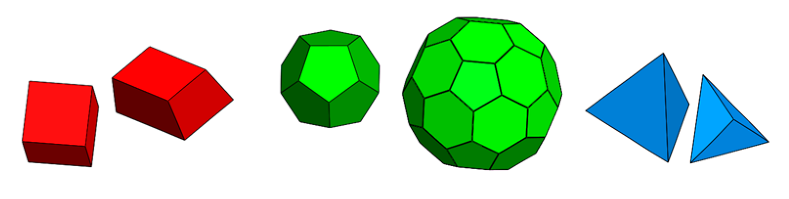
In fluid dynamics applications, it is the most desirable to divide the domain into hexahedral (HEX) control volumes (Figure 1—left) as the resulting mesh is characterized by low numerical diffusion. Unfortunately the numerical diffusion increases in the case of the flow not being perpendicular to the faces of control volumes and it is not always possible to construct a structured HEX mesh for complex geometries. Moreover, the generation of such a mesh usually requires high engineering skills and is a time-consuming task. Therefore this mesh type is usually ineffective in industrial applications due to the high cost of engineering time.
1.2.2. Tetrahedral Mesh
Semi-automatic tetrahedral (TETRA) mesh generation algorithms have been implemented into commercial pre-processors in order to overcome HEX mesh disadvantages. TETRAs (Figure 1—right) are the simplest volume elements as they consist of four faces. The faces are plane segments, thus both face and volume centroid locations are well defined. The unquestionable advantage of TETRA mesh is the ease of its generation even in the case of complicated geometry. On the other hand, TETRAs cannot be stretched excessively, so significantly larger numbers of elements have to be used in comparison to structured HEX mesh in order to achieve acceptable accuracy in representing certain spaces. Moreover, the neighbouring nodes of a TETRA element may lie in nearly one plane and therefore computing gradients can be difficult and lead to convergence problems [25]. In consequence, the numerical diffusion of TETRA mesh is significantly higher than HEX mesh and low-quality TETRAs result in convergence errors. The above-mentioned disadvantages contribute to a reduction of solution accuracy.
1.2.3. Polyhedral Mesh
The polyhedral (POLY) mesh (Figure 1—centre) was introduced in order to overcome the above-mentioned disadvantages of HEX and TETRA meshes and simultaneously combine the advantages of both types of the control volumes (low numerical diffusion of HEX and rapid semi-automatic generation of TETRA) [17,27,28,29].
The major benefit of POLY is that each individual cell has many neighbours (in contrast only four neighbours in case of TETRA elements), thus gradients can be approximated much better in comparison to TETRA. POLYs are also less sensitive to stretching than TETRAs which results in better numerical stability of the model. In some cases, POLY can even achieve better accuracy than HEX due to larger numbers of neighbouring elements allowing for an interchange of mass over a larger number of faces, reducing numerical diffusion effects caused by flows not perpendicular to any of the cell faces. This proves to be advantageous in situations where no prevailing flow direction can be identified and leads to a more accurate solution achieved with a lower cell count [17,29].
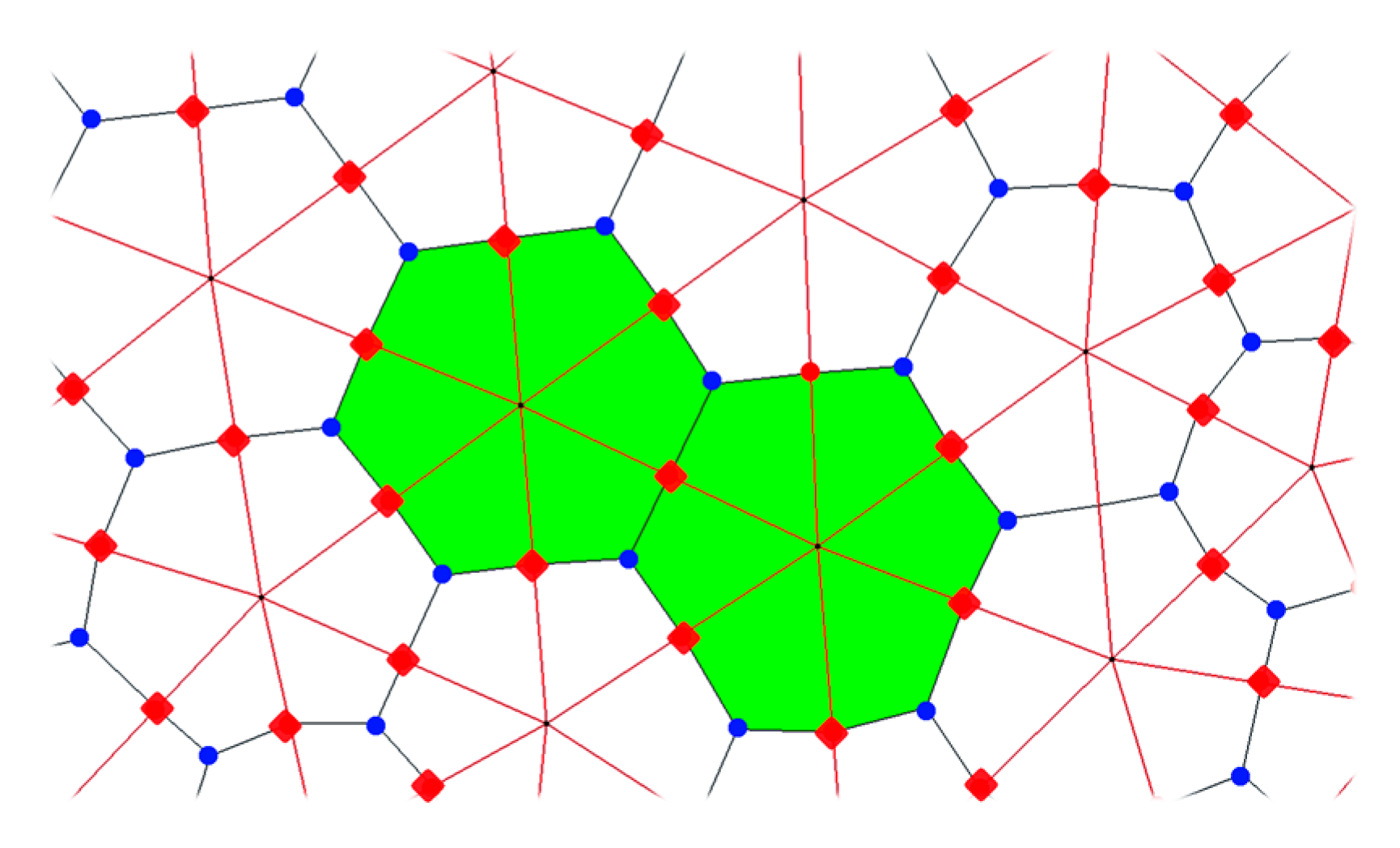
POLY mesh generation is a simple conversion of TETRAs to POLYs by decomposition of cells into multiple sub-volumes as illustrated in Figure 2. In order to do so, new edges are created on each face between the face centroid (dots in Figure 2) and the centroids of the edges of that face (diamonds in Figure 2). Subsequently, new faces are created within the cell by connecting the cell centroid to the new edges of each face. The newly-created faces may be adjusted and merged with the neighbouring faces during the agglomeration process in order to minimize the number of faces on the resultant polyhedral cell.
1.3. Numerical Accuracy
Numerical accuracy and its estimation is an important issue not only in CFD but also in broader areas of computational physics. Numerical errors resulting from an algorithm and mesh are difficult to be distinguished from physical modelling errors. The common practice of publishing comparisons based on coarse mesh solutions without systematic error testing is observed, although individual researchers strive to control numerical accuracy.
One issue connected with the numerical accuracy estimation is the iterative convergence: in most cases, it can be assumed that it is achieved with at least three orders of magnitude decrease in the normalized residuals for each equation solved.
The computational domain discretization resulting in mesh resolution is also a crucial factor influencing the solution of an analysed case. One such method for discretization error estimation is the Richardson Extrapolation (RE) [30]. The local RE values of predicted variables may not exhibit a monotonic dependence on mesh resolution. Moreover, in transient calculations, RE will also be a function of time and space. Despite its shortcomings and generalizations, it is currently the most reliable method available for the prediction of numerical uncertainty. The Grid Convergence Index (GCI) is based on the RE. It is recommended by the Fluids Engineering Division of the American Society of Mechanical Engineers to estimate the discretization error and was applied within this paper.
2. Methods
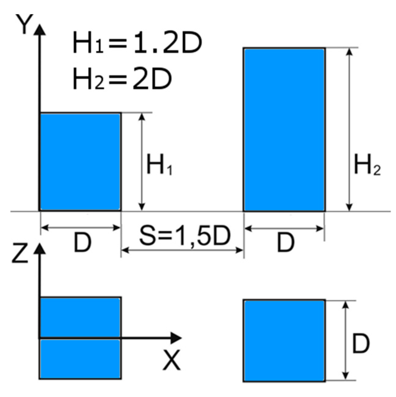
2.1. The Research Object
The research object represents a set of two buildings modelled as cuboids of square base and different heights settled in the flow domain. As depicted in Figure 3, the height ratio of the buildings models is 0.6 and the distance between them is set at 1.5 of the building base side length (D).
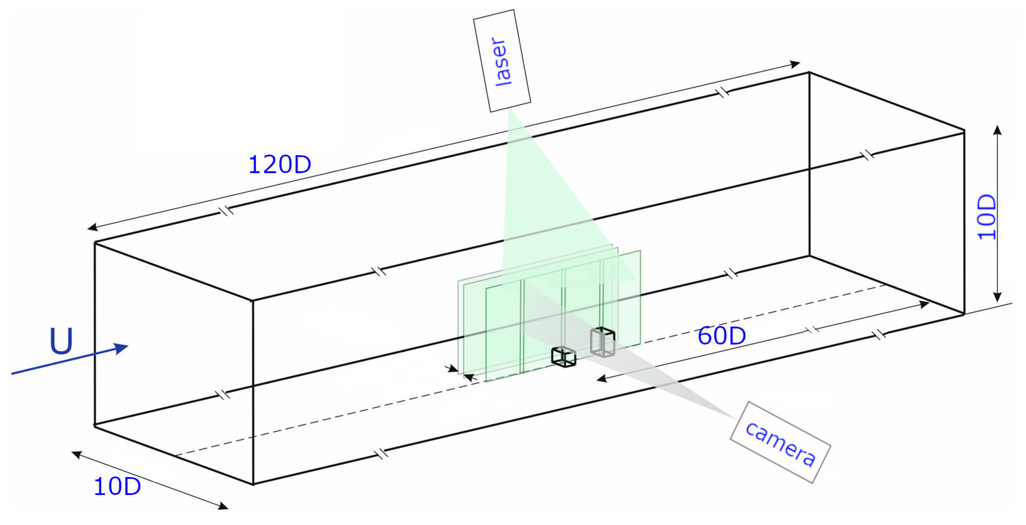
2.2. Experimental Research Using Particle Image Velocimetry
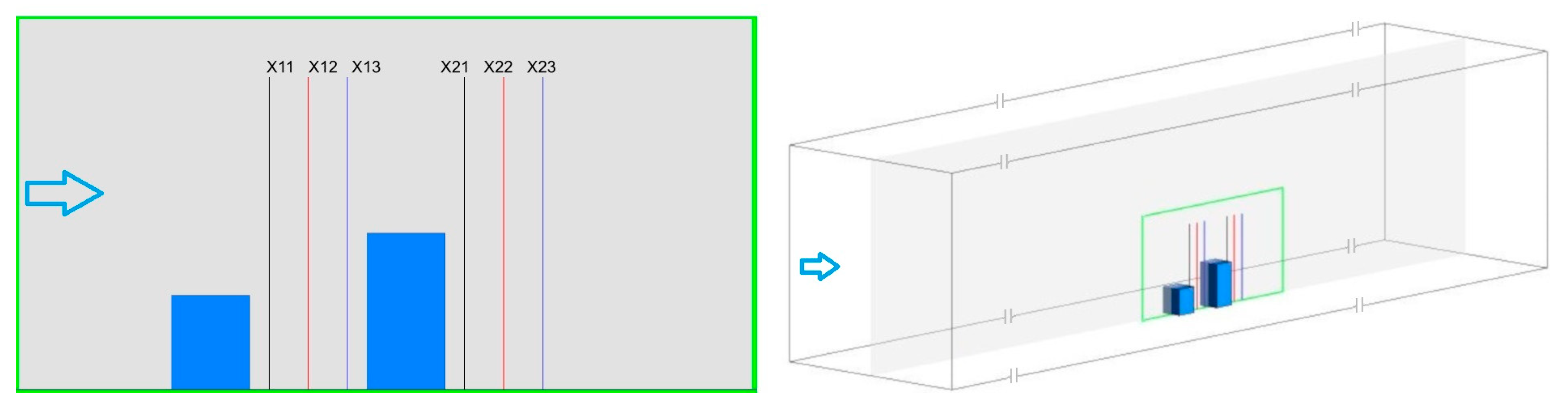
The experiment with the Particle Image Velocimetry (PIV) technique was carried out in the wind tunnel at the Institute of Thermomechanics of the Academy of Sciences of the Czech Republic. The measurements set-up is presented in Figure 4. The analysed configuration of building models was located within a ground boundary layer generated by the facility output from the contraction nozzle of a cross-section of 10D in width and 10D in height. The test section of the wind tunnel is 120D long but the measurements were performed in the central part of the tunnel. The lower building was placed 60D upstream the test section. A laser beam from a dual-head Nd:YLF laser with a pulse energy of 10 mJ at 2 kHz illuminated the particles. Dantec CCD camera (SpeedSense 611) was used to capture pairs of particle images at a frame rate of 100 Hz. The SAFEX fog generator was used to seed ~1 μm oil droplets. Seeding particles were introduced into the flow in a sufficient and stable concentration. The parameters of PIV experiments were set on the base of [31]. Instantaneous and time-averaged flow velocity fields were measured within the areas, marked in Figure 4 with green fields, lying in the plane Z = const. The PIV measurements provided the velocity vector field with two velocity components (Ux and Uy) in horizontal (X) and vertical (Y) direction. Time-averaged PIV results were used for comparison with CFD results.
2.3. Numerical Analysis
2.3.1. Pre-Processing
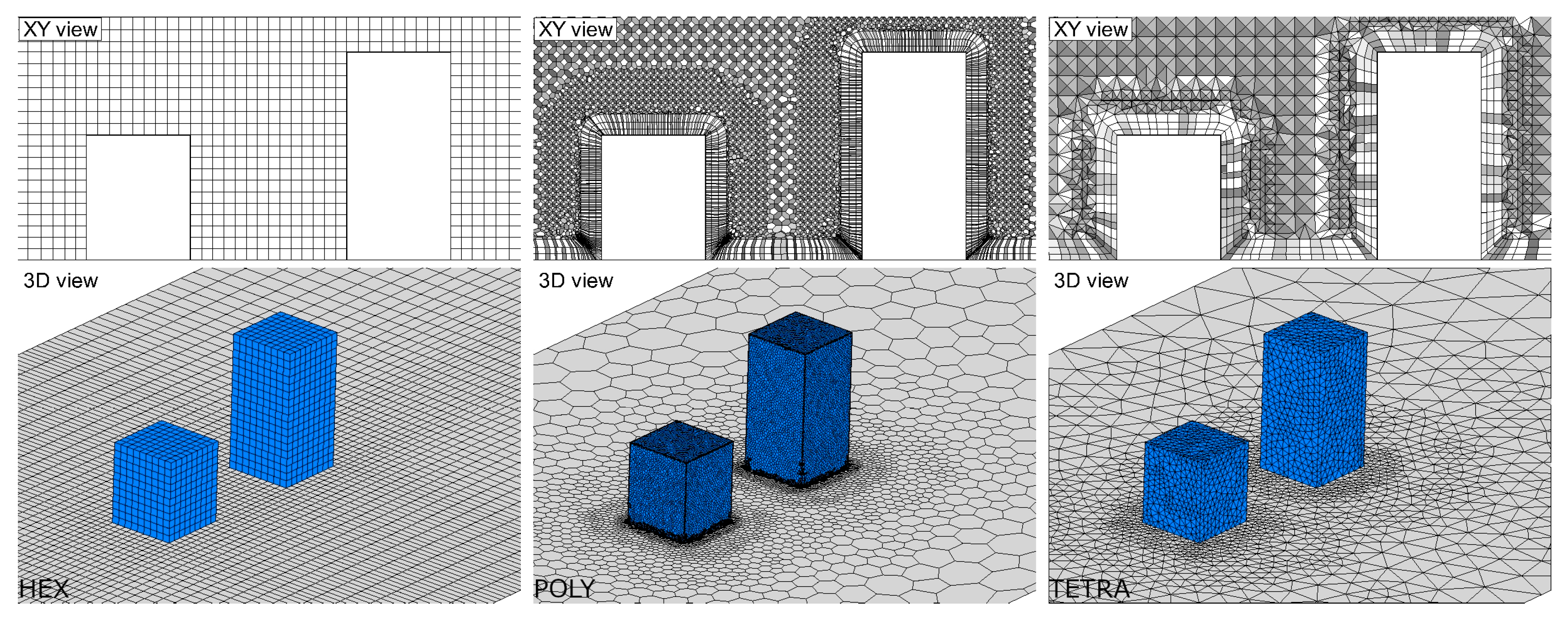
The computational domain represents the research object depicted in Figure 3 placed in a virtual wind tunnel domain of dimensions matching the experimental test section (Figure 4) of the wind tunnel. Moreover, the dimensions correspond with the best practise guidelines by [15]. The meshing was carried out using ICEM CFD 19.2 software. Three different mesh types were used (Figure 5): HEX, POLY and TETRA. For each mesh type, three meshes of different resolutions were generated in order to estimate the discretization error using the GCI method. The relative cell size was defined as the ratio of the average cell size (h) defined with Formula (1) and the base side length of the modelled building (D). Initially, HEX, POLY and TETRA meshes of the relative cell size h/D equal 0.32 were generated.
where:
- ΔVi—the volume of the ith cell,
- N—total number of cells in the computational domain.
The HEX mesh of h/D = 0.32 was prepared using the blocking technique in order to generate perfectly orthogonal cells. The domain was split into 42 blocks and edge parameters (number of nodes and node distribution along a specific edge) were defined for selected edges to control cell sizes distribution. The distribution of nodes along the edges of the modelled buildings was uniform and the node spacing was defined as D/10. The nods distribution away from the buildings was defined with a sophisticated approach described with Formula (2) with the first layer height equal to D/10. The defined edge parameters were copied to the parallel edges.
where:
- Si—distance from the node on the wall to node i,
- R—ratio limited by 0.25 < R < 4.0,
- n—total number of nodes along the edge.
The TETRA mesh was created using a top-down meshing approach (OCTREE algorithm) with prism layers. The mesh was intensively smoothed in order to meet the high mesh quality criteria. The mesh resolution was controlled by the global element seed size equal 2D and maximum element size on surfaces representing the walls of the modelled buildings equal D/10 with growth ratio equal to 1.2. The prism layer, which is state-of-the-art in industry, was applied in order to assure finer normal cell sizes perpendicular to the walls of the buildings and the bottom wall. The prism layer consisted of three individual layers of total height equal to D/5, growth ratio equal to 1.2 and exponential growth law.
The POLY mesh was obtained by converting the TETRA mesh of decreased relative cell size to POLY in Ansys Fluent 19.2 using the standard and fully automatic method described in the Section 1.2.3. Polyhedral mesh. Such procedure allowed to generate POLY meshes of the relative cell sizes matching the ones for HEX and TETRA meshes—0.32, 0.48, 0.64.
Subsequently, HEX, TETRA and POLY meshes of the relative cell size increased to h/D = 0.48 and finally to h/D = 0.64 were generated by proportional scaling the node distribution and nodes count of the initial meshes (h/D = 0.32).
2.3.2. Boundary Conditions and Numerical Model Parameters
The identical computational model (except for the mesh) was used for all cases analysed within the research. The solver was configured as pressure-based and analysis were performed for a steady state. A realizable k-epsilon viscous model according to [15,16] was applied along with enhanced wall treatment. The viscous model constants were given the following values: C2 Epsilon = 1.9, TKE Prandtl Number = 1 and TDR Prandtl Number = 1.3.
Velocity-inlet boundary condition type was assigned to the inlet of the computational domain with the use of the user-defined function (UDF). It was described by the velocity profile according to the Equation (3) [15] whereas the turbulence kinetic energy (k) and energy dissipation rate (ε) were defined on the basis of Equations (4) and (5) respectively and according to [32]. The values of the constants in Equations (3)–(5) were thoroughly investigated and validated during previous extensive research, therefore, the applied inlet profile corresponds with the inlet to the wind tunnel test section utilized within PIV research. All the measurements were carried out for the Reynolds number ReD = 9000 based on the free stream velocity U(δ) = 5.5 m/s.
where
- δ—the thickness of the ground layer (2D),
- U(δ)—free stream velocity (5.5 m/s),
- α—terrain type factor (0.15),
- u*—friction velocity (0.04 U(δ)),
- Cμ—constant (0.09),
- κ—von Karman constant (0.41).
The outlet of the computational domain was defined as pressure outlet with a gauge pressure of 0 Pa (operating pressure—101,325 Pa), backflow turbulent intensity of 5% and backflow turbulent viscosity ratio of 10. Wall no slip shear condition was assigned to the remaining surfaces. Pressure-velocity coupling by the SIMPLE algorithm was used as a solution method—this algorithm uses a relationship between velocity and pressure corrections to enforce mass conservation and to obtain the pressure field. The model convergence was defined on the basis of qualitative and quantitative monitoring of the residuals.
3. Results
3.1. Grid Convergence Index (GCI)
The GCI was calculated in order to minimize the discretization error. The grid refinement factor r was calculated based on the representative mesh size h (1) as:
Moreover, the following assumption was made:
k denotes the value of the variable important to the objective of the simulation study for solution obtained with the kth mesh. The average relative X velocity calculated for line X12 was selected as the above-mentioned variable (Figure 7 describes the location of the X12 line).
The approximate relative error was calculated on the basis of Equation (10).
Finally, the GCI was determined using Equation (11):
All the values of the above-defined quantities are listed in Table 1.
The obtained results indicate the mesh convergence in case of all analysed mesh types: HEX, POLY and TETRA.
3.2. Calculation Time
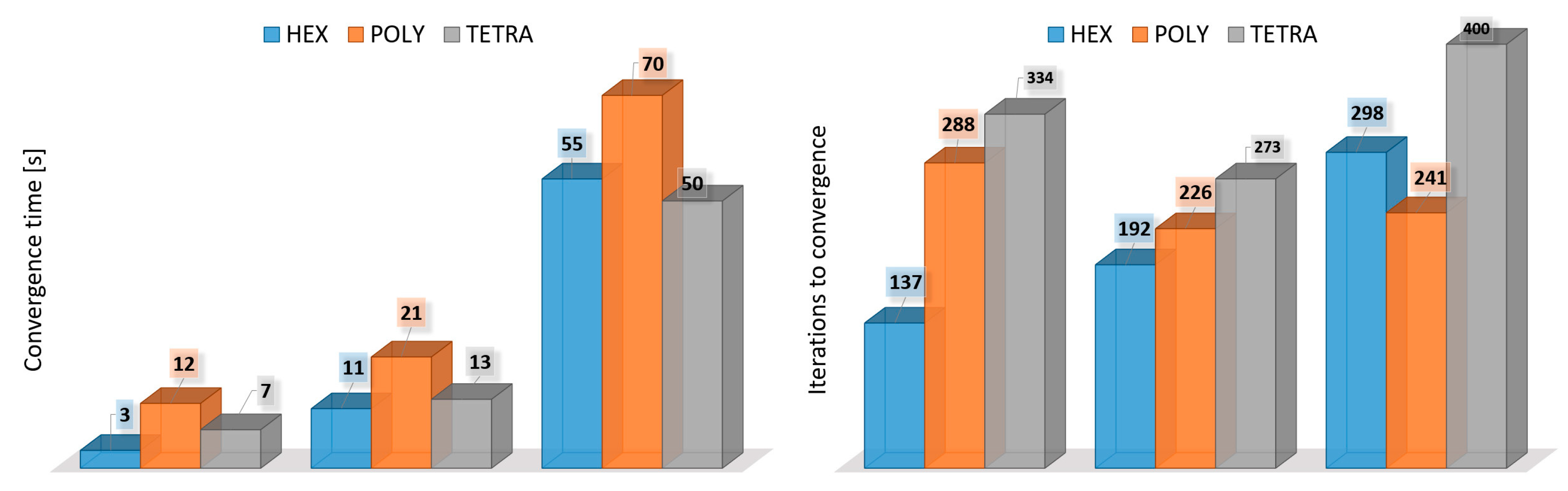
The numerical calculations were performed with Ansys Fluent 19.2 on Windows 10 workstation equipped with AMD Ryzen 7 2700X, 3700MHz CPU and 64GB of RAM. The solver was operating in parallel mode using 8 cores and 16 logical processors. The calculation time (Figure 6—left) and the number of iterations to convergence (Figure 6—right) were given as the solver output.
3.3. Velocity Profile
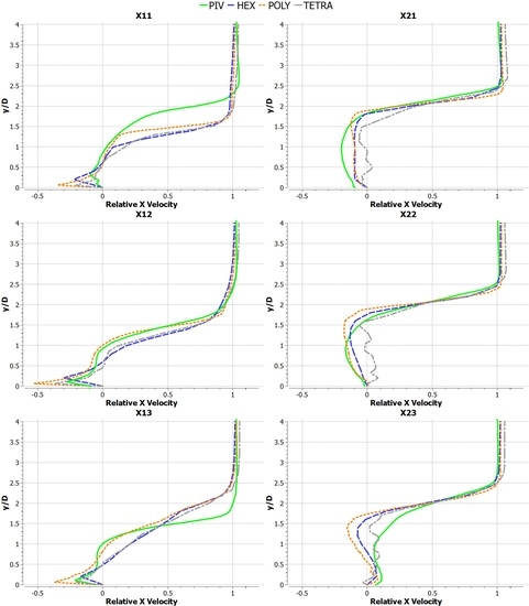
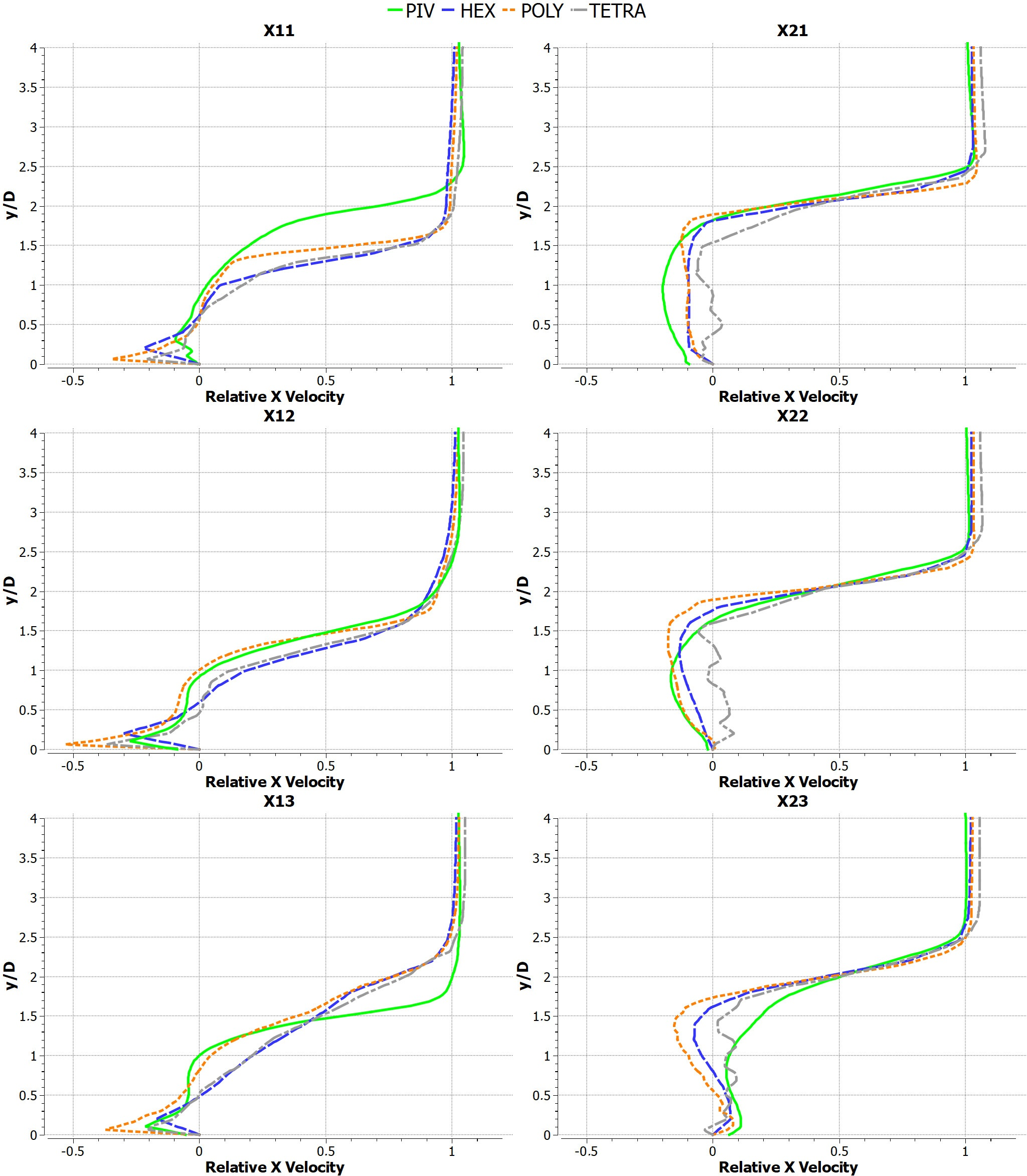
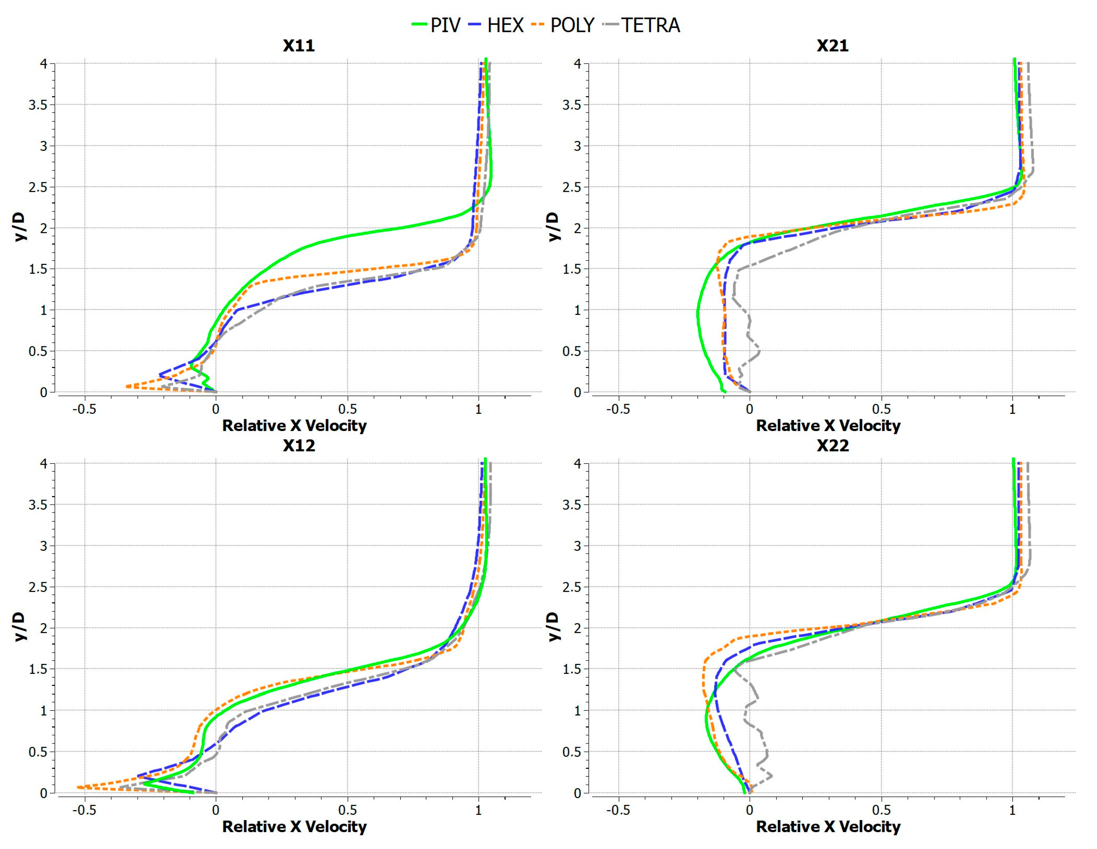
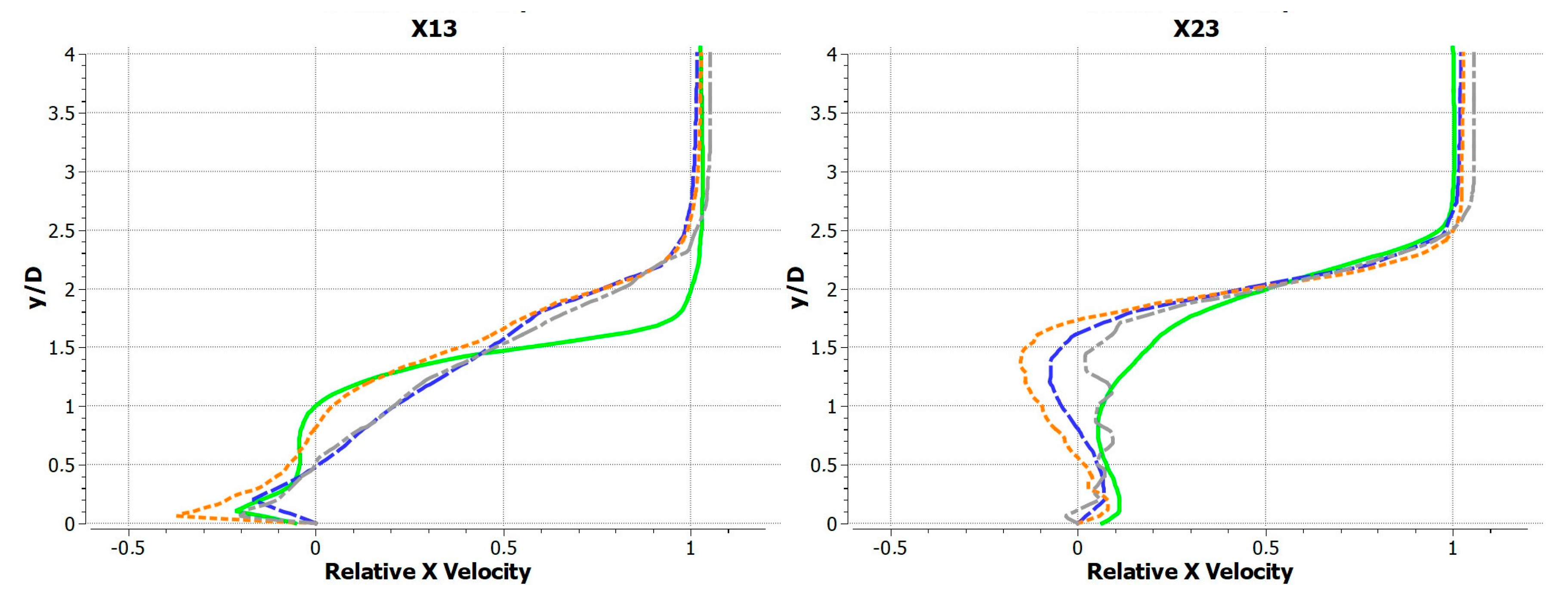
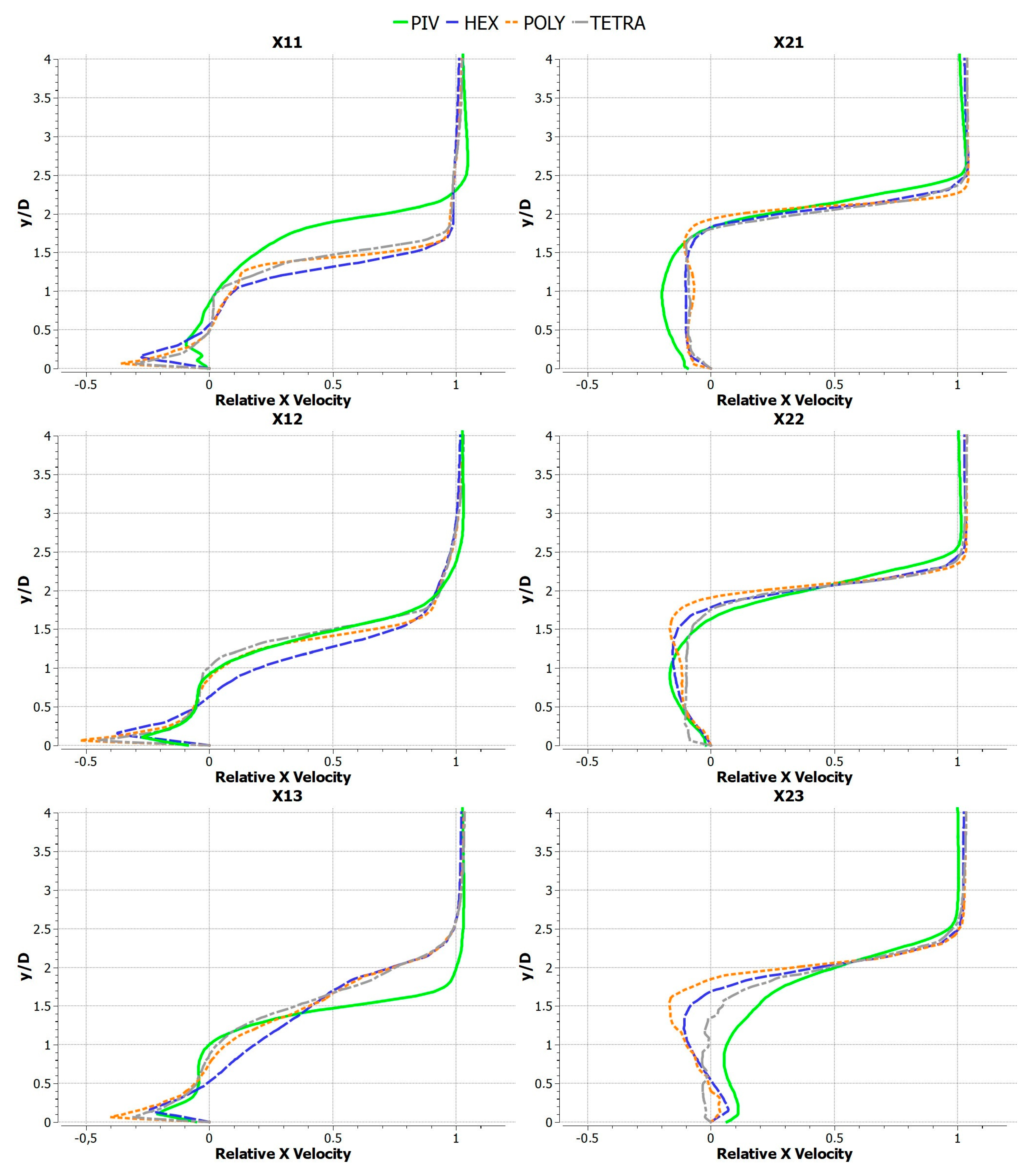
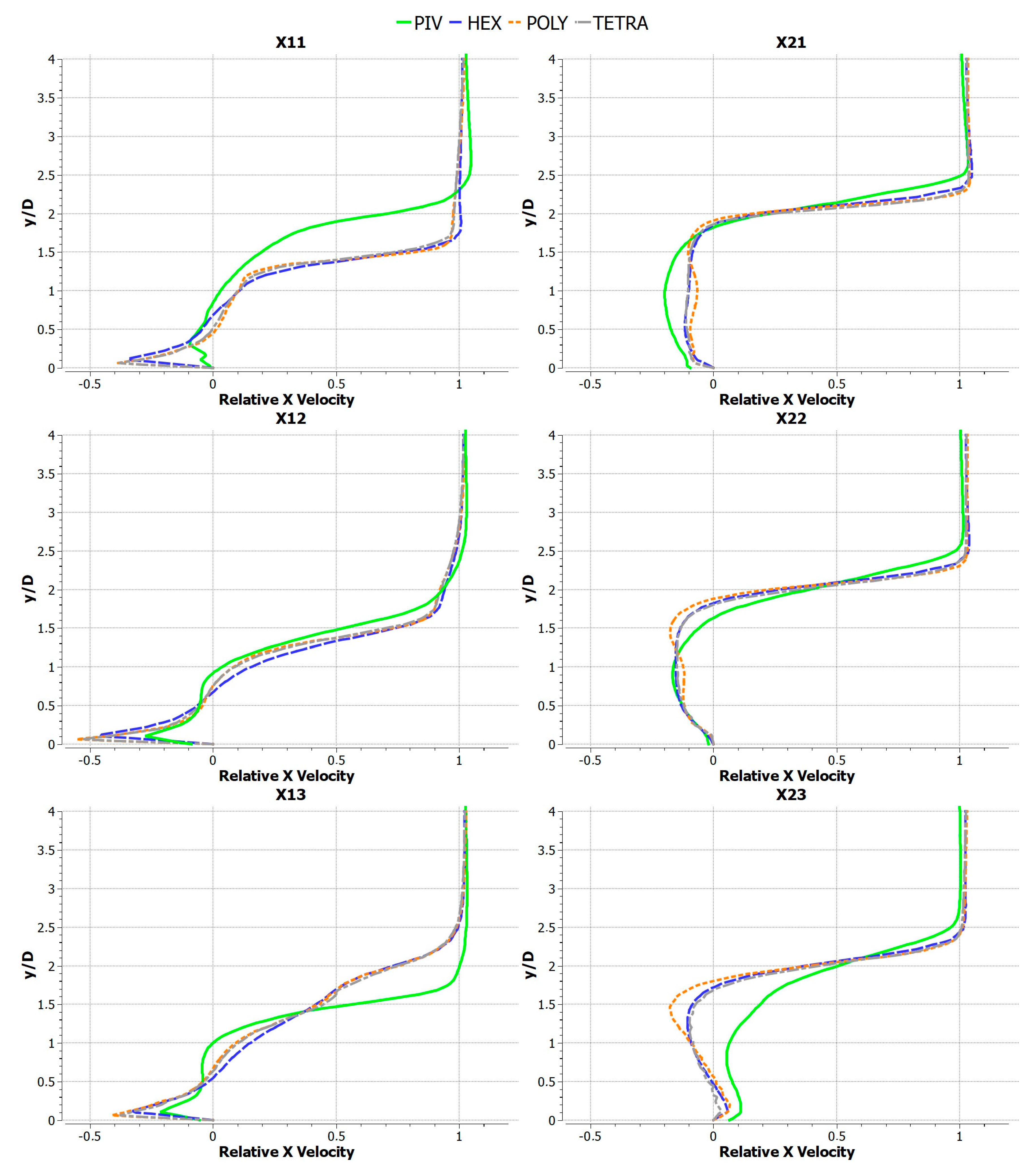
The relative horizontal (X) velocity is the velocity component along the horizontal (X) axis of the domain (parallel to the inflow) divided by the inflow velocity value above the boundary layer which for the analysed cases was 5.5 m/s. The profiles are depicted for the results obtained with the use of time-averaged PIV and for the results of the numerical analysis carried out for the three mesh types and three relative cell sizes.
The relative horizontal (X) velocity profiles are calculated along the Xij lines located in the midplane (Z = 0) of the domain as shown in Figure 7. Line X11 is situated 0.25D downstream the back of the first building whereas lines X12 and X13 are located 0.75D and 1.25D respectively. Similarly, line X21 is situated 0.25D, line X22—0.75D and line X23—1.25D downstream the back of the second building. The vertical extent of the lines was calculated as y/D <0.4>.
3.4. Velocity Field
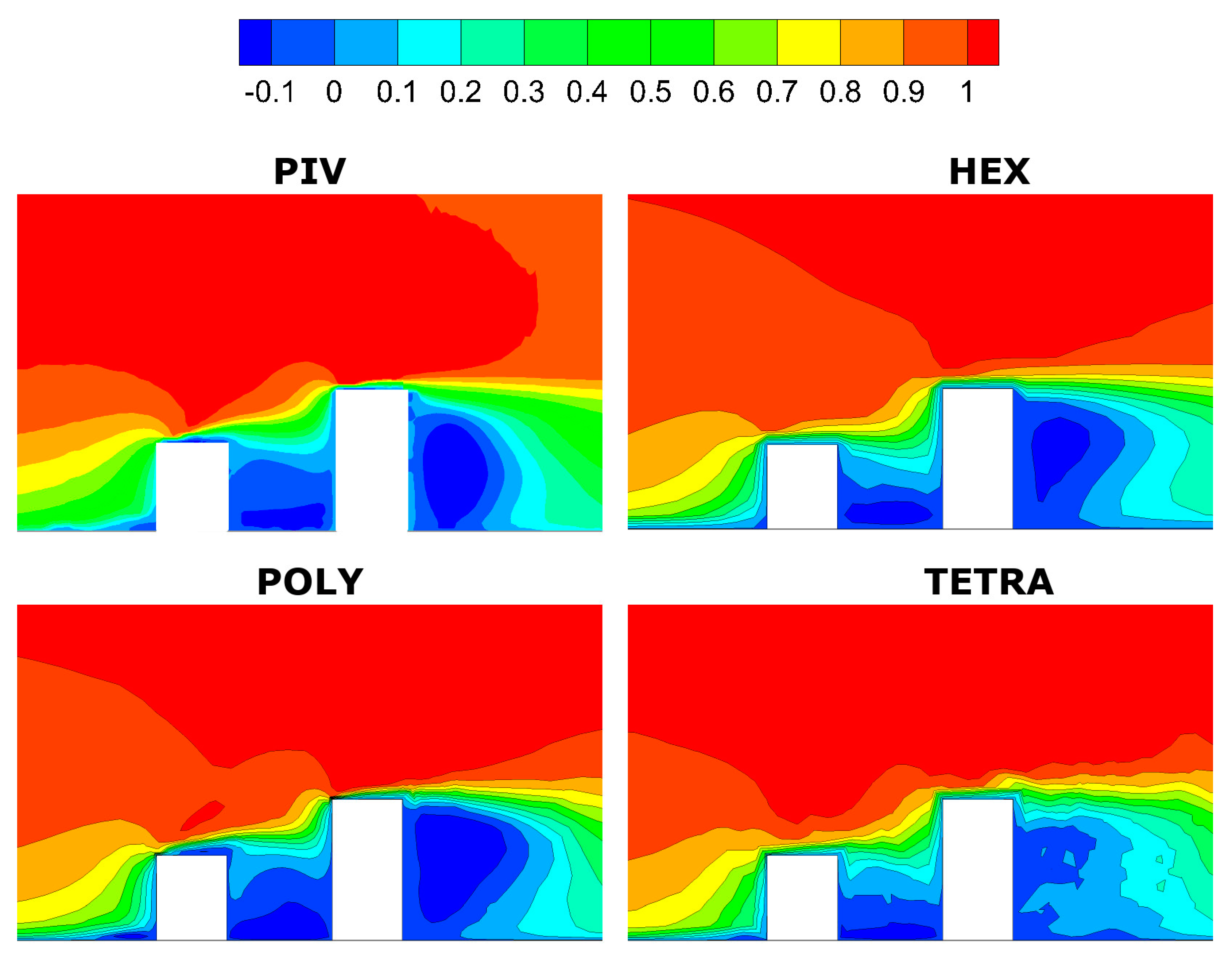
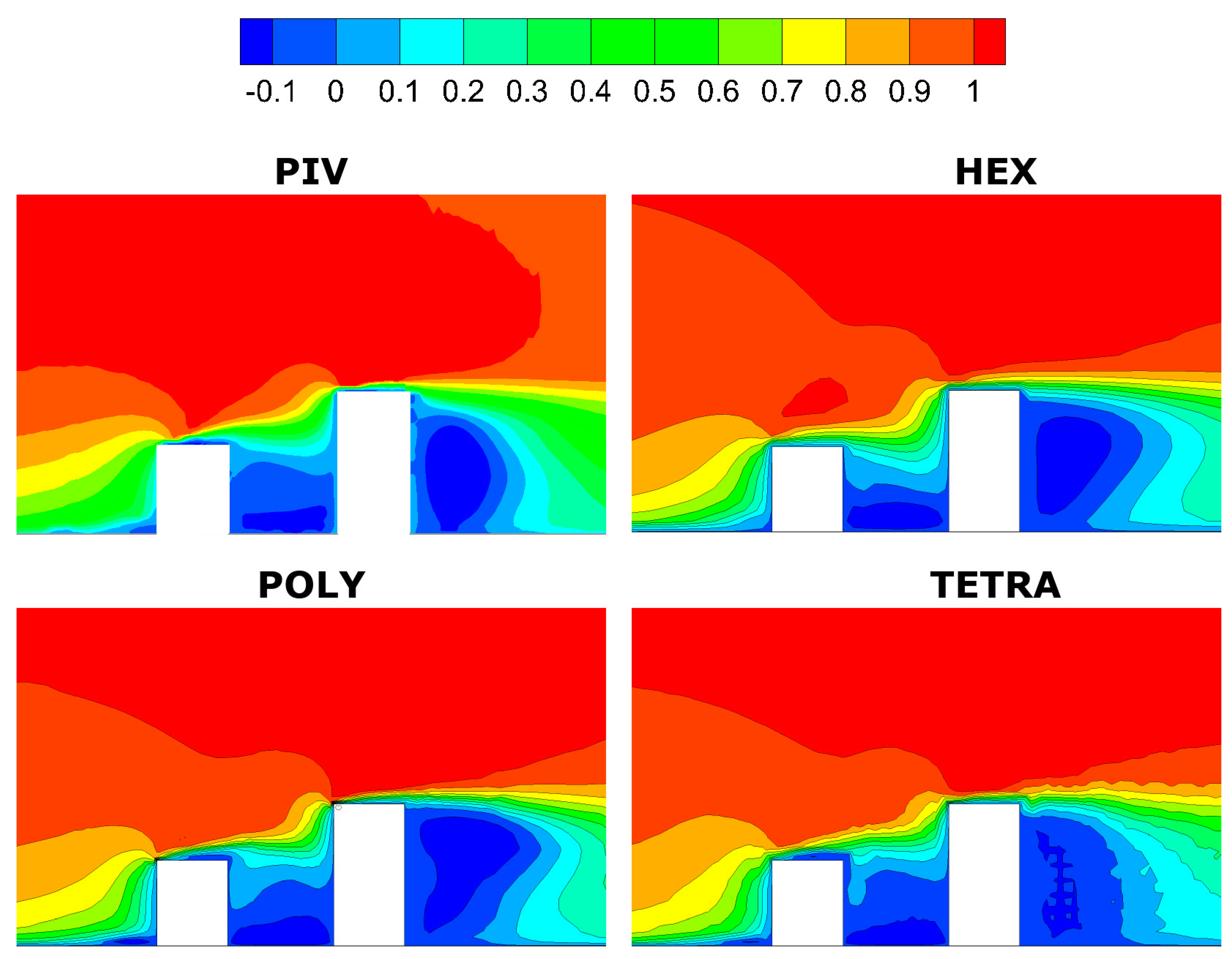
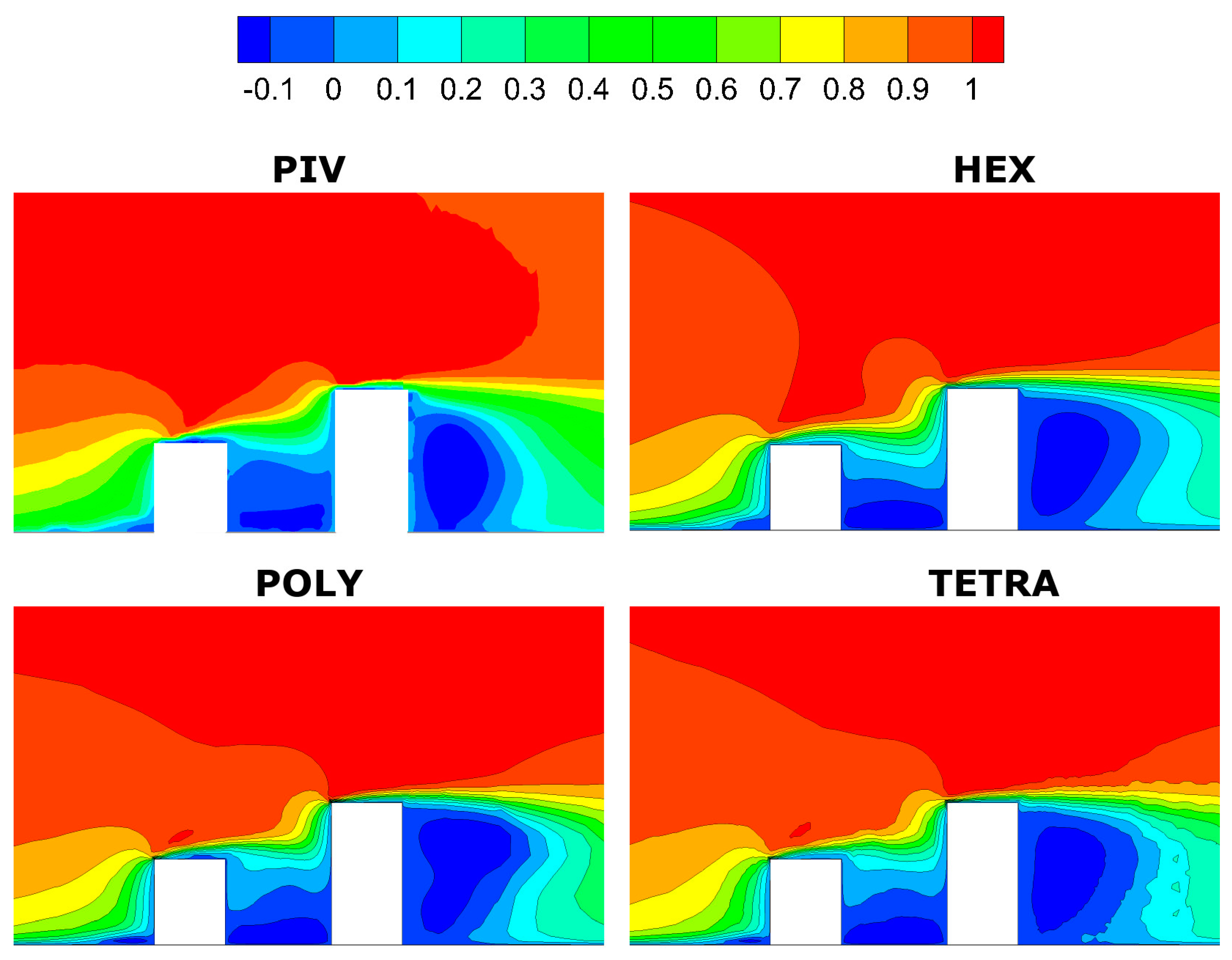
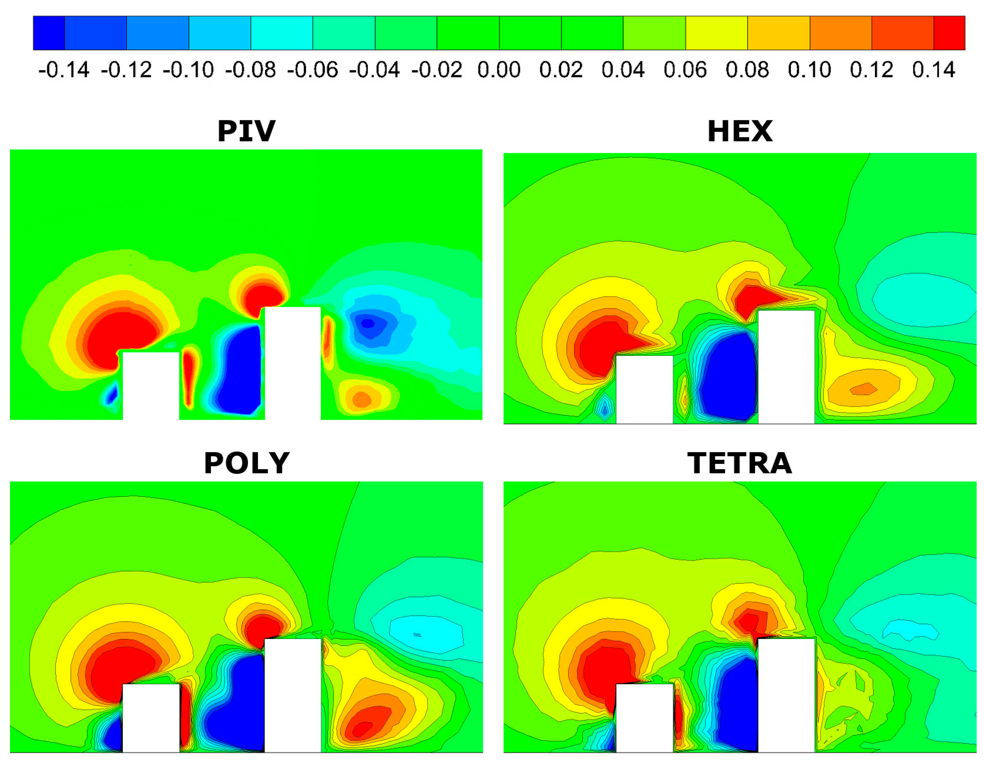
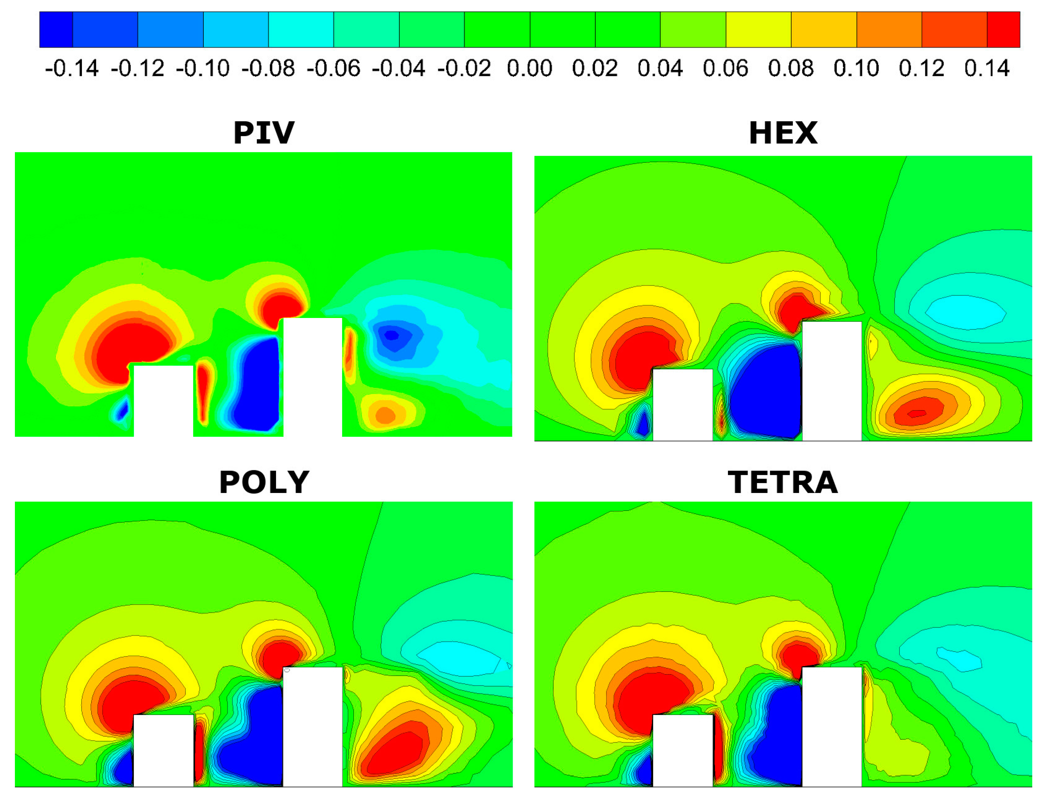
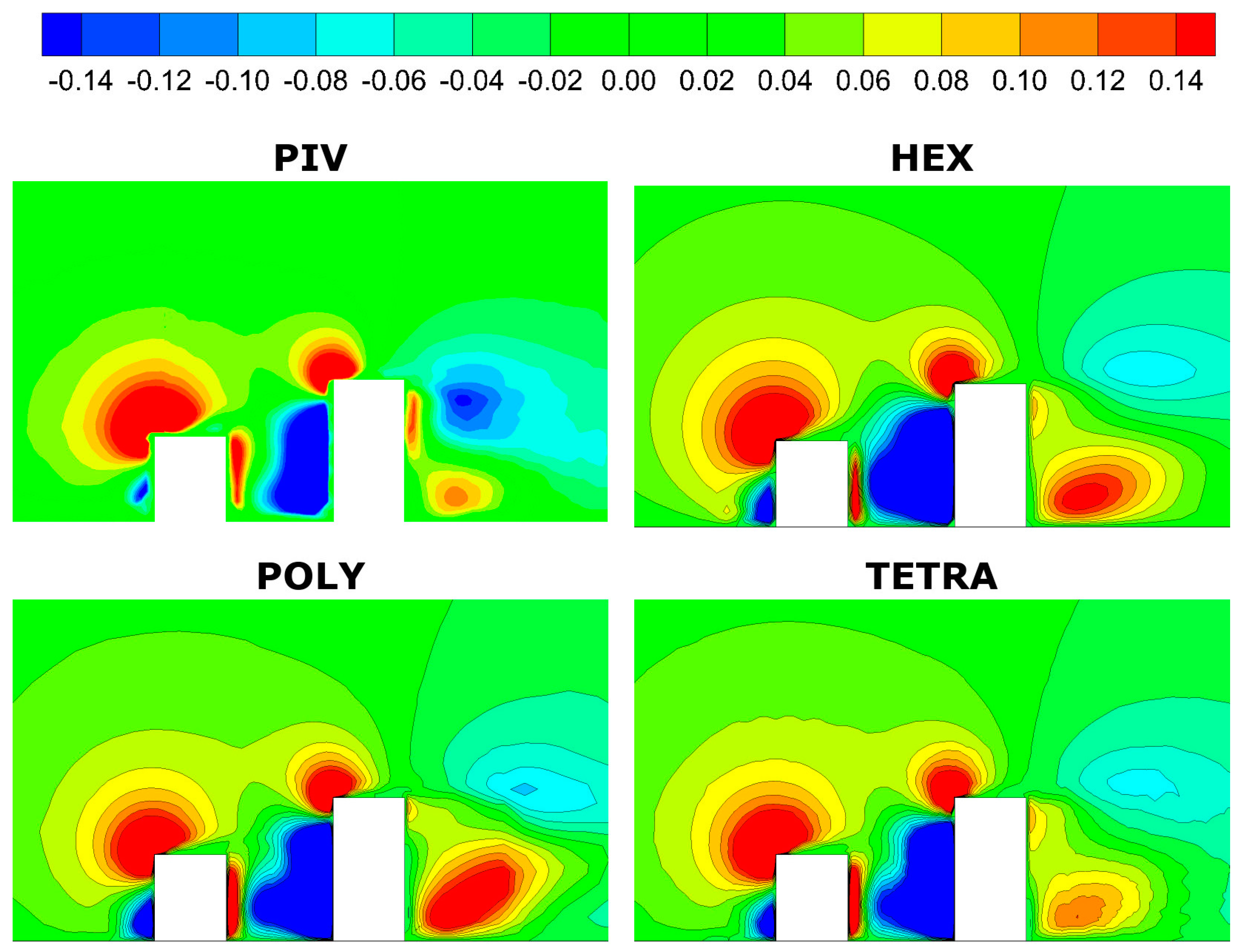
The relative horizontal (X) velocity field (velocity component parallel to the inflow) and the relative vertical (Y) velocity field (velocity component perpendicular to the inflow) are depicted in Figure 11, Figure 12 and Figure 13 and Figure 14, Figure 15 and Figure 16 for each of the analysed mesh types and relative cell sizes in midplane (Z = 0) for the extent of X <2D, 7.5D> and Y <0, 4.8D>.
4. Discussion
The mesh convergence analysis was carried out with the use of the GCI method, which is recommended by the Fluids Engineering Division of the American Society of Mechanical Engineers to estimate the discretization error. Three sets of meshes characterized by different relative cell sizes were generated for each of the analysed mesh type (HEX, POLY, TETRA) in order to define mesh convergence and the GCI. The mesh convergence was achieved for each of the analysed mesh types but the GCI for the HEX mesh was the lowest (0.76%) while it was almost three times more in case of TETRA mesh (2.19%). POLY mesh, with GCI = 1.36%, turned out to be advantageous in comparison to TETRA although the prevalence of HEX mesh is unquestionable. The iterations count to convergence of CFD analysis was lower for POLY in comparison to TETRA by 14% (h/D = 0.64), 17% (h/D = 0.48) and 40% (h/D = 0.32). HEX mesh needed the least iterations to achieve convergence of the model except for the case of the lowest relative cell sizes where POLY mesh was the best of all the mesh types. The above-mentioned characteristics did not translate directly to calculation time as each iteration for POLY mesh lasted longer in comparison to both HEX and TETRA meshes. Therefore the analysis with POLY mesh lasted for the longest time for all relative cell sizes. The calculation time was the lowest in case of HEX mesh for relative cell sizes equal 0.48 and 0.64 and in case of TETRA mesh for relative mesh size equal 0.32.
The results concerning the relative horizontal (X) velocity profiles for all mesh types and all relative cell sizes indicate very good conformity with PIV data above y/D = 2.0, that is above the taller building. The most significant discrepancies occur close to the ground (bottom wall) approx. up to y/D = 0.3. The differences can be observed not only between the PIV and CFD but also among CFD results for different mesh types. In case of the coarsest meshes (h/D = 0.64), POLY generated too intensive reversed flow between the buildings (X11, X12, X13), while HEX mesh results were the most comparable to PIV. One of the reasons for the above-mentioned differences between PIV and CFD can be the roughness of the wind tunnel’s bottom wall which was not taken into account in the CFD analysis. The differences between the results for the individual mesh types can be justified by the influence of the mesh type characteristics (i.e., numerical diffusivity) as the thickness of the prism layer was identical in case of POLY and TETRA. POLY mesh seems to be the most comparable to PIV for y/D <0.3, 2.0> in the area between the two buildings (X11, X12, X13). Results for POLY and HEX are comparable to PIV behind the second building, especially for X21 and X22. These meshes over predict the reversed flow for X23. The results for TETRA mesh behind the second building for y/D < 2.0 and h/D = 0.64 do not correspond with PIV as well as CFD for HEX and POLY. Very similar conclusions can be drawn for relative cell size equal 0.48 but POLY and TETRA results are more comparable to each other than it was for h/D = 0.64. Moreover, results for TETRA behind the second building (especially for X21 and X22) are in better agreement with PIV as well as with CFD for HEX and POLY. The discrepancies between PIV and CFD results in case of the finest meshes (h/D = 0.32) are, in general, similar as for the coarser meshes (h/D = 0.48 and 0.64) but the differences between the mesh types are less intensive. POLY and TETRA results are almost in a perfect match between the buildings while HEX and TETRA results are more consistent after the second building.
The in-depth analysis of the relative horizontal (X) velocity field indicates an acceptable qualitative agreement of the PIV and CFD results although quantitative differences are noticeable. The velocity gradients just above the upper walls of the buildings obtained with POLY mesh seem to be more comparable to PIV then HEX mesh results. It can be caused by the finer normal cell sizes towards and perpendicular to the wall (prism layer) applied in case of POLY and TETRA—structured and perfectly orthogonal HEX mesh is not so flexible in such cases. TETRA results for the meshes of h/D = 0.64 and 0.48 are characterized by unphysical (jagged) velocity contours, which require an individual post-processing approach to be better visualized. The influence of mesh size on the results is the most visible in case of TETRA and the least visible in case of POLY and HEX. Similar findings can be applied to relative vertical (Y) velocity fields but the velocity field near the back wall of the first building obtained with POLY mesh (regardless of the relative mesh size) best corresponds to PIV results.
5. Conclusions
The research concerns a very complex flow problem [33] and the purpose of the carried out analysis was to indicate the influence of the discretization of the computational domain representing the tandem building arrangement in an urban environment on CFD results, particularly the velocity field in the direct vicinity of the modelled objects. Three mesh types (HEX, POLY and TETRA) were analysed and the GCI was calculated for each of them based on three meshes of different relative cell sizes. The research proved the prevalence of HEX mesh in terms of time necessary to obtain a converged solution as well as the consistency of the CFD and experimental results. Moreover, HEX mesh was one of the lowest GCI (0.76%). On the other hand, this type of mesh needs significantly greater engineering skills as well as time to be generated and therefore is not popular in industrial applications, especially for initial analysis concerning complex geometries. The comparison of results generated with POLY and TETRA does not allow to indicate the more favourable one as each mesh type is advantageous in certain aspects. TETRA mesh generates the converged solution faster but results obtained with POLY mesh are less dependent on the relative cell size. The carried out research proved the importance and crucial significance of pre-processing on CFD results and indicated POLY mesh as one of the possible choices in computational domain discretization. The results obtained within this study will be beneficial to researchers and engineers in selecting the optimal method of computational domain discretization, which directly impacts the CFD results.
Author Contributions
Conceptualization, M.S., R.G. and K.G.; Methodology, M.S. and R.G.; Software, M.S. and K.G.; Validation, R.G.; Formal Analysis, M.S., R.G. and J.K.; Investigation, M.S. and R.G.; Resources, M.S., R.G. and K.G.; Data Curation, M.S. and A.J.; Writing-Original Draft Preparation, M.S. and R.G.; Writing-Review & Editing, M.S. and R.G.; Visualization, M.S.; Supervision, M.S. and R.G.; Project Administration, M.S. and R.G.; Funding Acquisition, M.S. and R.G.
Funding
This research was partially funded by the National Science Centre of Poland (Narodowe Centrum Nauki) grant number 2017/01/X/ST8/00019 and 2017/01/X/ST8/00076.
Conflicts of Interest
The authors declare no conflict of interest.
References
- Gnatowska, R. Numerical Method for Detection of Wind Discomfort in Built Environment. Part 1. Recent Adv. Res. Environ. Effects Build. People 2010, 217–224. [Google Scholar]
- Gnatowska, R. Development of Local Wind Climate as an Element of Rural Planning. Teka Kom. Ochr. Kszt. Środ. Przyr. Oddz. 2010, 7, 97–102. [Google Scholar]
- Koss, H.H. On differences and similarities of applied wind comfort criteria. J. Wind Eng. Ind. Aerodyn. 2006, 94, 781–797. [Google Scholar] [CrossRef]
- Willemsen, E.; Wisse, J.A. Design for wind comfort in The Netherlands: Procedures, criteria and open research issues. J. Wind Eng. Ind. Aerodyn. 2007, 95, 1541–1550. [Google Scholar] [CrossRef]
- Blocken, B. 50 years of Computational Wind Engineering: Past, present and future. J. Wind Eng. Ind. Aerodyn. 2014, 129, 69–102. [Google Scholar] [CrossRef]
- Gnatowska, R. Aerodynamic Characteristics of Three-Dimensional Surface-Mounted Objects in Tandem Arrangement. Int. J. Turbo Jet-Engines 2011, 28, 21–29. [Google Scholar] [CrossRef]
- Gnatowska, R. Application of model methods in designing and modernization of built-up areas. Civ. Environ. Eng. Rep. 2012, 9, 41–50. [Google Scholar]
- Martinuzzi, R.J.; Havel, B. Vortex shedding from two surface-mounted cubes in tandem. Int. J. Heat Fluid Flow 2004, 25, 364–372. [Google Scholar] [CrossRef]
- Martinuzzi, R.J.; Havel, B. Turbulent flow around two interfering surface-mounted cubic obstacles in tandem arrangement. J. Fluids Eng. Trans. Asme 2000, 122, 24–31. [Google Scholar] [CrossRef]
- Abd Razak, A.; Hagishima, A.; Ikegaya, N.; Tanimoto, J. Analysis of airflow over building arrays for assessment of urban wind environment. Build. Environ. 2013, 59, 56–65. [Google Scholar] [CrossRef]
- Blocken, B.; Stathopoulos, T.; van Beeck, J. Pedestrian-level wind conditions around buildings: Review of wind-tunnel and CFD techniques and their accuracy for wind comfort assessment. Build. Environ. 2016, 100, 50–81. [Google Scholar] [CrossRef] [Green Version]
- Blocken, B. Computational Fluid Dynamics for urban physics: Importance, scales, possibilities, limitations and ten tips and tricks towards accurate and reliable simulations. Build. Environ. 2015, 91, 219–245. [Google Scholar] [CrossRef] [Green Version]
- Blocken, B.; Gualtieri, C. Ten iterative steps for model development and evaluation applied to Computational Fluid Dynamics for Environmental Fluid Mechanics. Environ. Model. Softw. 2012, 33, 1–22. [Google Scholar] [CrossRef]
- Blocken, B.; Janssen, W.D.; van Hooff, T. CFD simulation for pedestrian wind comfort and wind safety in urban areas: General decision framework and case study for the Eindhoven University campus. Environ. Model. Softw. 2012, 30, 15–34. [Google Scholar] [CrossRef]
- Tominaga, Y.; Mochida, A.; Yoshie, R.; Katoka, H.; Nozu, T.; Yoshikava, M.; Shirashava, T. AIJ guidelines for practical applications of CFD to pedestrian wind environment around buildings. J. Wind Eng. Ind. Aerodyn. 2008, 96, 1749–1761. [Google Scholar] [CrossRef]
- Gnatowska, R.; Sosnowski, M.; Uruba, V. CFD modelling and PIV experimental validation of flow fields in urban environments. E3S Web Conf. 2017, 14, 01034. [Google Scholar] [CrossRef] [Green Version]
- Sosnowski, M.; Krzywanski, J.; Gnatowska, R. Polyhedral meshing as an innovative approach to computational domain discretization of a cyclone in a fluidized bed CLC unit. E3S Web Conf. 2017, 14, 01027. [Google Scholar] [CrossRef] [Green Version]
- Sosnowski, M. Computational domain discretization in numerical analysis of flow within granular materials. In Proceedings of the 24th International Conference on Experimental Fluid Mechanics (EFM), Mikulov, Czech Republic, 14–17 May 2007. [Google Scholar]
- Krzywanski, J.; Nowak, W. Artificial Intelligence Treatment of SO2 Emissions from CFBC in Air and Oxygen-Enriched Conditions. J. Energy Eng. 2016, 142, 04015017. [Google Scholar] [CrossRef]
- Krzywanski, J.; Nowak, W. Modeling of bed-to-wall heat transfer coefficient in a large-scale CFBC by fuzzy logic approach. Int. J. Heat Mass Transf. 2016, 94, 327–334. [Google Scholar] [CrossRef]
- Jamrozik, A.; Tutak, W.; Kociszewski, A.; Sosnowski, M. Numerical simulation of two-stage combustion in SI engine with prechamber. Appl. Math. Model. 2013, 37, 2961–2982. [Google Scholar] [CrossRef]
- Jamrozik, A.; Tutak, W.; Gnatowski, A.; Gnatowska, R.; Winczek, J.; Sosnowski, M. Modeling of thermal cycle CI engine with multi-stage fuel injection. Adv. Sci. Technol. Res. J. 2017, 11, 179–186. [Google Scholar] [CrossRef]
- Gnatowska, R.; Sosnowski, M. The influence of distance between vehicles in platoon on aerodynamic parameters. in International Conference on Experimental Fluid Mechanics (EFM). Eur. Phys. J. Conf. 2017, 180, 194–198. [Google Scholar]
- Sosnowski, M. Computer aided optimization of a nozzle in around-the-pump fire suppression foam proportioning system. In Proceedings of the 23rd International Conference Engineering Mechanics 2017, Svratka, Czech Republic, 15–18 May 2017; pp. 914–917. [Google Scholar]
- Spiegel, M.; Redel, T.; Zhang, J.T.; Strufferd, T.; Hornegger, J.; Grossman, R.G.; Doerfeler, A.; Karmonik, C. Tetrahedral vs. polyhedral mesh size evaluation on flow velocity and wall shear stress for cerebral hemodynamic simulation. Comput. Methods Biomech. Biomed. Eng. 2011, 14, 9–22. [Google Scholar] [CrossRef] [PubMed]
- Morris, P.D.; Narracott, A.; von Tengg-Kobligk, H.; Silva Soto, D.A.; Hsiao, S.; Lungu, A.; Evans, P.; Bressloff, N.W.; Lawford, P.V.; Hose, D.R.; et al. Computational fluid dynamics modelling in cardiovascular medicine. Heart 2016, 102, 18–28. [Google Scholar] [CrossRef] [PubMed]
- Lanzafame, R.; Mauro, S.; Messina, M. Wind turbine CFD modeling using a correlation-based transitional model. Renew. Energy 2013, 52, 31–39. [Google Scholar] [CrossRef]
- Su, J.W.; Gu, Z.; Chen, C.; Xu, X.Y. A two-layer mesh method for discrete element simulation of gas-particle systems with arbitrarily polyhedral mesh. Int. J. Numer. Methods Eng. 2015, 103, 759–780. [Google Scholar] [CrossRef]
- Sosnowski, M.; Krzywanski, J.; Grabowska, K.; Gnatowska, R. Polyhedral meshing in numerical analysis of conjugate heat transfer. International Conference on Experimental Fluid Mechanics (EFM). EPJ Web Conf. 2018, 180, 02096. [Google Scholar] [CrossRef]
- Celik, I.B. Procedure for estimation and reporting of uncertainty due to discretization in CFD applications. J. Fluids Eng. Trans. Asme 2008, 130, 078001. [Google Scholar]
- Melling, A. Tracer particles and seeding for particle image velocimetry. Meas. Sci. Technol. 1997, 8, 1406–1416. [Google Scholar] [CrossRef]
- Richards, P.; Hoxey, R.; Short, L. Wind pressures on a 6 m cube. J. Wind Eng. Ind. Aerodyn. 2001, 89, 1553–1564. [Google Scholar] [CrossRef]
- Gnatowska, R. Wind-induced pressure loads on buildings in tandem arrangement in urban environment. Environ. Fluid Mech. 2018, 18, 1–20. [Google Scholar] [CrossRef]
Figure 1.
Hexahedral (left), polyhedral (centre) and tetrahedral (right) control volumes.

Figure 2.
TETRA to POLY conversion.

Figure 3.
The research object.

Figure 4.
Sketch of the experimental test stand.

Figure 5.
The section of the computational domain discretized with the use of HEX, POLY and TETRA elements.
Figure 5.
The section of the computational domain discretized with the use of HEX, POLY and TETRA elements.

Figure 6.
Convergence time (left) and iterations count to convergence (right) of the analysed cases.
Figure 6.
Convergence time (left) and iterations count to convergence (right) of the analysed cases.

Figure 7.
Post-processing lines for the velocity profiles.

Figure 8.
Relative horizontal (X) velocity profiles for time-averaged PIV and CFD (h/D = 0.64).


Figure 9.
Relative horizontal (X) velocity profiles for time-averaged PIV and CFD (h/D = 0.48).

Figure 10.
Relative horizontal (X) velocity profiles for time-averaged PIV and CFD (h/D = 0.32).

Figure 11.
Relative horizontal (X) velocity field for time-averaged PIV and CFD (h/D = 0.64).

Figure 12.
Relative horizontal (X) velocity field for time-averaged PIV and CFD (h/D = 0.48).

Figure 13.
Relative horizontal (X) velocity field for time-averaged PIV and CFD (h/D = 0.32).

Figure 14.
Relative vertical (Y) velocity field for time-averaged PIV and CFD (h/D = 0.64).

Figure 15.
Relative vertical (Y) velocity field for time-averaged PIV and CFD (h/D = 0.48).

Figure 16.
Relative vertical (Y) velocity field for time-averaged PIV and CFD (h/D = 0.32).


Table 1.
Mesh parameters and values of quantities calculated based on Equations (1), (6)–(12).
| Mesh Type | h/D [-] | N [-] | [-] | h [-] | r [-] | [-] | [-] | p [-] | ea [%] | GCI [%] |
|---|---|---|---|---|---|---|---|---|---|---|
| HEX | 0.32 | 352,971 | 0.6452 | 8 | 1.4320 | 0.009 | converged | 3.2879 | 1.38% | 0.76% |
| 0.48 | 120,204 | 0.6541 | 12 | 1.3701 | 0.002 | |||||
| 0.64 | 46,736 | 0.6563 | 16 | - | - | |||||
| POLY | 0.32 | 350,779 | 0.6556 | 8 | 1.4410 | −0.042 | converged | 5.3027 | 6.47% | 1.36% |
| 0.48 | 117,234 | 0.6132 | 12 | 1.3279 | −0.004 | |||||
| 0.64 | 50,064 | 0.6096 | 16 | - | - | |||||
| TETRA | 0.32 | 329,615 | 0.6404 | 8 | 1.4002 | 0.021 | converged | 3.1619 | 3.33% | 2.19% |
| 0.48 | 120,064 | 0.6617 | 12 | 1.3533 | 0.006 | |||||
| 0.64 | 48,448 | 0.6679 | 16 | - | - |
© 2019 by the authors. Licensee MDPI, Basel, Switzerland. This article is an open access article distributed under the terms and conditions of the Creative Commons Attribution (CC BY) license (http://creativecommons.org/licenses/by/4.0/).
Share and Cite
MDPI and ACS Style
Sosnowski, M.; Gnatowska, R.; Grabowska, K.; Krzywański, J.; Jamrozik, A. Numerical Analysis of Flow in Building Arrangement: Computational Domain Discretization. Appl. Sci. 2019, 9, 941. https://doi.org/10.3390/app9050941
AMA Style
Sosnowski M, Gnatowska R, Grabowska K, Krzywański J, Jamrozik A. Numerical Analysis of Flow in Building Arrangement: Computational Domain Discretization. Applied Sciences. 2019; 9(5):941. https://doi.org/10.3390/app9050941
Chicago/Turabian StyleSosnowski, Marcin, Renata Gnatowska, Karolina Grabowska, Jarosław Krzywański, and Arkadiusz Jamrozik. 2019. "Numerical Analysis of Flow in Building Arrangement: Computational Domain Discretization" Applied Sciences 9, no. 5: 941. https://doi.org/10.3390/app9050941
Note that from the first issue of 2016, this journal uses article numbers instead of page numbers. See further details here.