Research on the Influence of Backlash on Mesh Stiffness and the Nonlinear Dynamics of Spur Gears
by
Yangshou Xiong
1,2,*, 
Kang Huang
3,*,
Fengwei Xu
3,†,
Yong Yi
3,†,
Meng Sang
3,† and
Hua Zhai
4,† 1
School of Materials Science and Engineering, Hefei University of Technology, Hefei 230009, China
2
Anhui Zhongke Photoelectric Color Selection Machinery Co., Ltd., Hefei 231202, China
3
School of Mechanical Engineering, Hefei University of Technology, Hefei 230009, China
4
Institute of Industry & Equipment Technology, Hefei University of Technology, Hefei 230009, China
*
Authors to whom correspondence should be addressed.
†
These authors contributed equally to this work.
Appl. Sci. 2019, 9(5), 1029; https://doi.org/10.3390/app9051029
Submission received: 26 December 2018
/
Revised: 4 March 2019
/
Accepted: 7 March 2019
/
Published: 12 March 2019
(This article belongs to the Special Issue Optical High-speed Information Technology)
Abstract
:In light of ignoring the effect of backlash on mesh stiffness in existing gear dynamic theory, a precise profile equation was established based on the generating processing principle. An improved potential energy method was proposed to calculate the mesh stiffness. The calculation result showed that when compared with the case of ignoring backlash, the mesh stiffness with backlash had an obvious decrease in a mesh cycle and the rate of decline had a trend of decreasing first and then increasing, so a stiffness coefficient was introduced to observe the effect of backlash. The Fourier series expansion was employed to fit the mesh stiffness rather than time-varying mesh stiffness, and the stiffness coefficient was fitted with the same method. The time-varying mesh stiffness was presented in terms of the piecewise function. The single degree of freedom model was employed, and the fourth order Runge–Kutta method was utilized to investigate the effect of backlash on the nonlinear dynamic characteristics with reference to the time history chart, phase diagram, Poincare map, and Fast Fourier Transformation (FFT) spectrogram. The numerical results revealed that the gear system primarily performs a non-harmonic-single-periodic motion. The partially enlarged views indicate that the system also exhibits small-amplitude and low-frequency motion. For different cases of backlash, the low-frequency motion sometimes shows excellent periodicity and stability and sometimes shows chaos. It is of practical guiding significance to know the mechanisms of some unusual noises as well as the design and manufacture of gear backlash.
1. Introduction
Gear dynamics is an important method to predict dynamic performance as well as to monitor the status of a gear system. The time-varying mesh stiffness caused by alternately changing the gear pairs in mesh plays a crucial role in dynamic responses. An effective time-varying mesh stiffness model is a basic condition to conduct a dynamic analysis. Thus, it is significant to recognize the mechanism of a gear system’s shock and vibration to investigate the influence of time-varying mesh stiffness on vibration responses, especially with regard to the mechanism of the noise, which is hard to identify.
One consistently popular topic in gear dynamics is how to describe the change rule of time-varying mesh stiffness correctly and effectively. The ISO Standard 6336-1 [1] recommends a stiffness formula to calculate the maximum single tooth mesh stiffness for spur and helical gears according to experimental tests. In References [2,3,4], time-varying mesh stiffness was simplified as a rectangular equation which had significant differences from the actual value. The authors in Reference [5] used a polynomial fitting method to smooth the result of the time-varying contact stiffness that was obtained by the Hertz contact algorithm. The Fourier series was used to fit time-varying mesh stiffness function approximatively in Reference [6]. Kuang and Yang proposed an equation to calculate the single tooth bending stiffness for the addendum-modified gear and the curve-fitted coefficients took the number of teeth as a variable [7]. In Reference [8], the mesh stiffness between an engaged gear pair was regarded as consisting of local Hertzian stiffness and tooth bending stiffness. Cai and Tang revised Kuang’s calculation formula and proposed an analytical method to calculate the mesh stiffness by considering the load condition and the tooth profile modification in References [9,10]. Chen investigated the differences between the rectangular stiffness and its approximate form on the gear nonlinear dynamic characteristics in Reference [11].
According to the available literature, the main methods to calculate mesh stiffness are Finite Element Method (FEM) and the potential energy method. These two methods have advantages and disadvantages. The potential energy method was proposed by Yang [12] and has been improved several times [13,14,15,16]. It is widely used in the failure analysis of a gear system [17,18,19,20,21]. The FEM, which can reflect the real contact status, is often applied to figure out engineering problems [22,23,24]. Moreover, the FEM is a common method to verify the validity of the potential energy method while both the FEM and potential energy method always ignore the influence of backlash on mesh stiffness.
The backlash is very useful to avoid the jam phenomenon in conditions of elastic deformation and thermal expansion, i.e., adaptive backlash is one of the necessary conditions to ensure the normal operation of gear. One way to achieve backlash is to reduce tooth thickness. The reduction in tooth thickness will cause a decrease in the stiffness, further influencing the dynamic performance. In current gear dynamics, the effect of backlash is limited to the definition of the nonlinear backlash function [25,26,27,28,29,30].
Thus, this work will focus on the influence of backlash on time-varying mesh stiffness, carry out nonlinear dynamic analysis, and investigate the dynamic responses for various values of backlash. This is expected to establish the indirect relationship between backlash and dynamic performance as well as direct the design and control of the gear’s backlash.
2. Influence of Backlash on Time-Varying Mesh Stiffness
2.1. Mesh Stiffness Model with Backlash
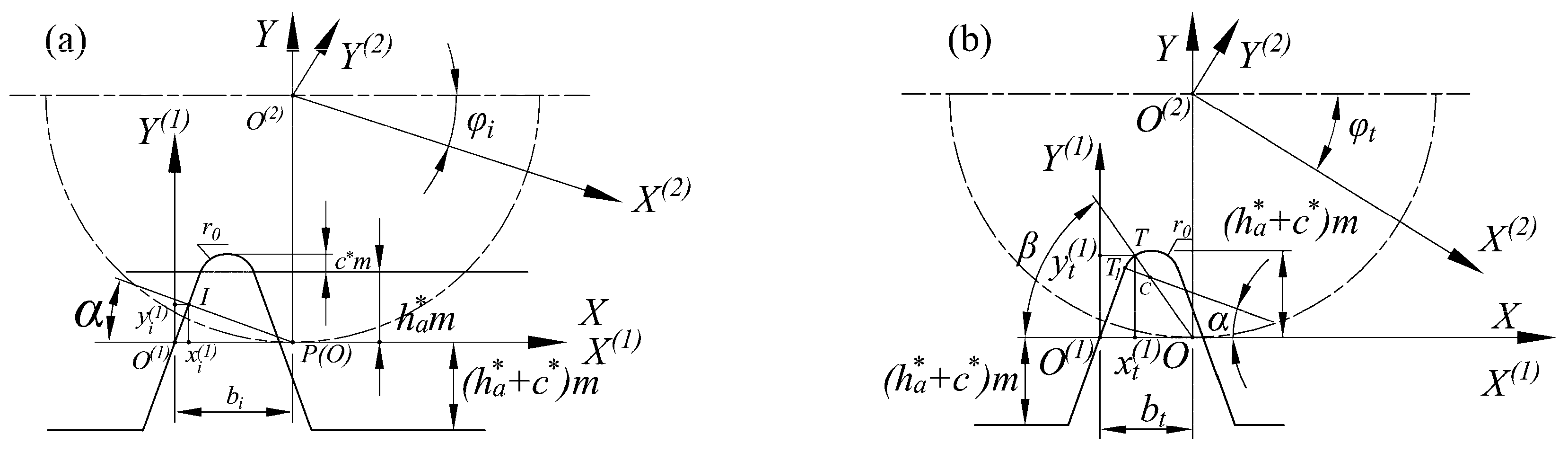
Available mesh stiffness models do not consider the influence of backlash. Precision tooth profile equations play an important role in the analysis method to calculate the mesh stiffness. According to the generating method of gear cutting, the tooth profile equations consist of two parts: the involute and transition curve, as shown in Figure 1.
The subscripts and in Figure 1 denote the involute curve and transition curve.
Equations of the involute curve are expressed as
where is defined as the contact point of the rack cutter and gear blank, and , .
The relationship between the pressure angle of the arbitrary point at the involute curve and can be deduced by
which can be simplified as
The value of for the involute start point is , Thus, the range of is
Equations of the transition curve are expressed as
where , , , , .
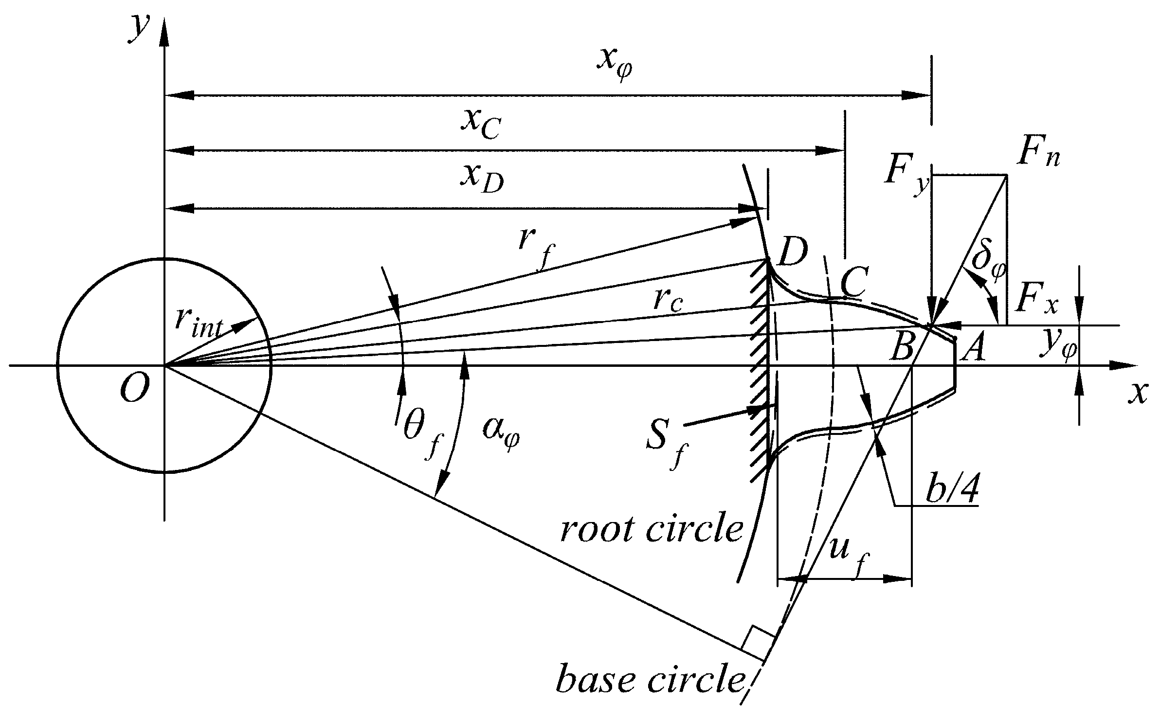
Then, the tooth profile, as shown in Figure 2, can be obtained by the new tooth profile equations as follows:
Here, , where represents the backlash, Z represents the tooth number, and it is assumed that the gear and pinion have the same value as the reduction in the thickness of the tooth.
According to the potential energy method, the potential energy deposited in the gear set can be divided into Hertzian energy , bending energy , shear energy , axial compressive energy , and fillet foundation energy . The relationship between the potential energy and corresponding stiffness can be expressed as follows:
where , , , , and denote the Hertzian contact stiffness, bending stiffness, shear stiffness, axial compressive stiffness, and fillet foundation stiffness, respectively. The stiffness contribution of the gear body is omitted [31].
Then, the total potential energy for a pair of teeth can be achieved by summing the energy components, i.e.,
Then, the single-tooth-pair mesh stiffness for a pair of spur gears with a contact ratio between 1 and 2 can be expressed as follows:
where the subscripts represent the gear and the pinion.
According to Reference [32], the Hertzian contact stiffness can be expressed as
where is Young’s modulus; is the tooth width; and is the Poisson’s ratio.
The fillet foundation stiffness can be calculated according to [13]
where is the angle between normal force and axis in Figure 2. The parameters can be calculated according to the following equation:
where , and are described in Figure 2, and are listed in Table 1.
According to cantilever beam theory, axial compressive energy, bending energy, and shear energy can be calculated by
where , , , , .
Further, the bending stiffness , shear stiffness , and axial compressive stiffness can be expressed as
2.2. Influence of Backlash on Stiffness
The backlash can be obtained by decreasing the thickness of the tooth or by increasing the center distance. Here, only the former situation will be discussed.
According to ISO/TR 10064-2-1996, the value of minimum backlash can be expressed as
where is the center distance.
In this paper, three cases will be discussed, i.e., Case 1: ; Case 2: ; Case 3: .
The parameters of an example gear pair are listed in Table 2.
According to the above-mentioned mesh stiffness model, the single-tooth-pair mesh stiffness and time-varying mesh stiffness can be calculated, as shown in Figure 3 and Figure 4.
By introducing a stiffness coefficient ,
where is the single-tooth-pair mesh stiffness for different values of backlash, a better view can be obtained to present the effect of backlash on stiffness, as shown in Figure 5.
Compared to Case 1, Case 2 and Case 3 shows an obvious reduction in single stiffness and mesh stiffness according to Figure 5. Moreover, the reduction is not proportionate. Compared with Case 1, the rate of decline for Case 2 and Case 3 shows a trend of decreasing first and then increasing in a mesh cycle from coming into the mesh to going out of the mesh.
2.3. Mesh Stiffness Fitting Method
In many studies, time-varying mesh stiffness is fitted in the form of the Fourier series expansion [33,34]. Despite being fitted by a high-level Fourier series, the difference between time-varying mesh stiffness and the fitting one is still very obvious in the alternate mesh area for single and double teeth. Here, the single-tooth-pair mesh stiffness, rather than the time-varying mesh stiffness, will be expressed in the form of the Fourier series expansion:
where is the mean value of the single-tooth-pair mesh stiffness. , are the amplitudes of the th order harmonic. is the stiffness fitting frequency when the mesh period is .
Similarly, the stiffness coefficient can also be expressed in the form of Fourier series expansion:
where is the mean value of the stiffness coefficient, are the amplitudes of the th order harmonic. is the coefficient fitting frequency when the mesh period is .
For the example gear pair, it can be found that the fitting effect is very well when , . The corresponding parameters are listed in Table 3.
Moreover, , , and can be further expressed as functions of backlash:
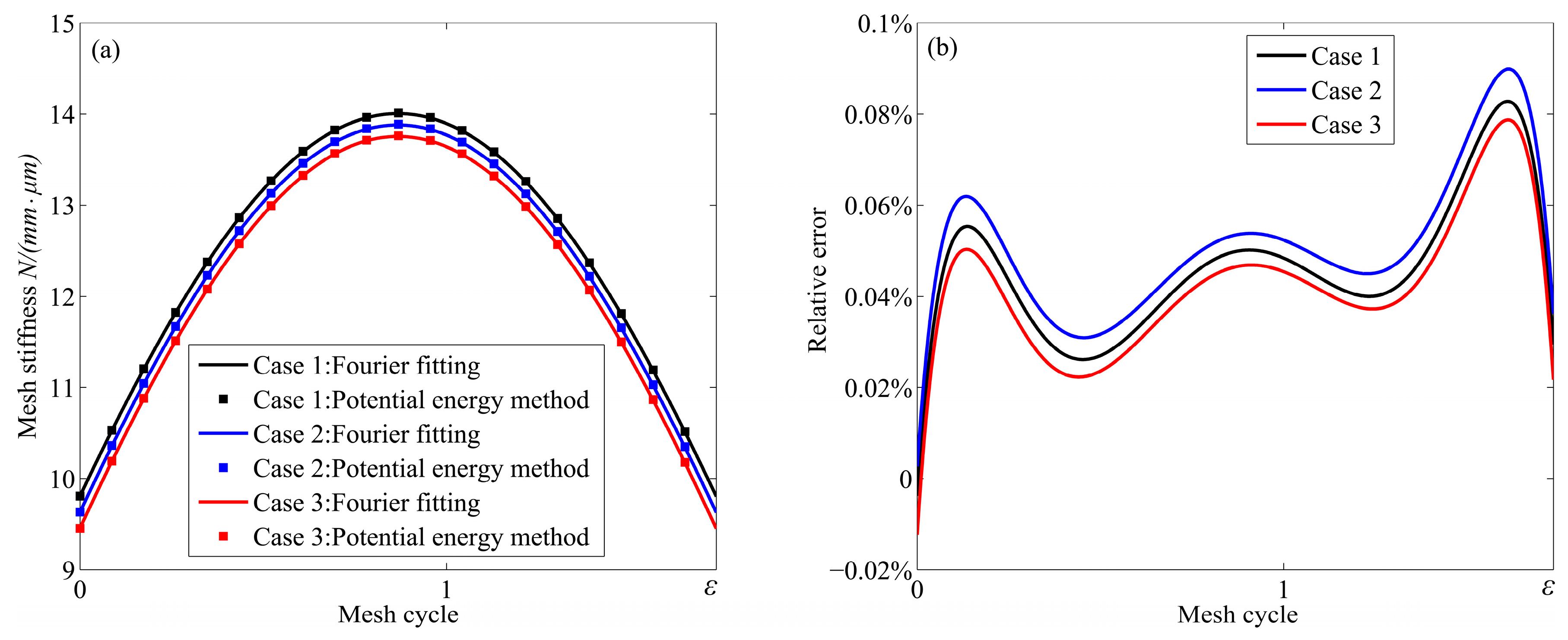
The fitting results are shown in Figure 6a:
According to Figure 6b, the relative error is less than 0.1%, which means the Fourier fitting has high precision.
Then, the time-varying mesh stiffness can be obtained by defining two pairs of teeth in mesh. In the meshing process of a gear set with a contact ratio between 1 and 2, as shown in Figure 7, the meshing teeth pair with the contact point located between point A and point C is defined as pair #1, and the meshing teeth pair with the contact point located between point C and point D is defined as pair #2.
The piecewise stiffness functions can be expressed as
3. Influence of Backlash on Dynamics
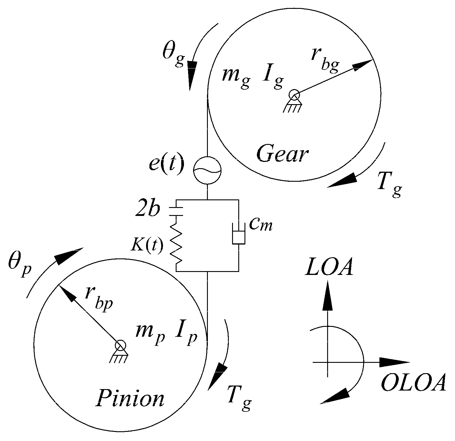
3.1. Single-Degree-of-Fredom(SDOF) Model and Dynamic Differential Equation
The SDOF model is shown in Figure 8. Two gears are combined with supporting shafts, which are regarded as rigid bodies with large support stiffness. The influences of friction and radial support are ignored. The pinion and gear are represented by their base circle radii of and , respectively. Then, the equations of motion can be expressed as follows:
where and represent the polar mass moments of inertia, respectively. and represent the masses of pinion and gear. represents the time-varying mesh stiffness. represents viscous damping, and represents the damping ratio. represents the static transmission error. and represent the input and output torques acting on the pinion and gear. To simplify the calculation, the fluctuations of input and output torque are neglected. The backlash function ‘’ can be expressed as
By employing dynamic transmission error , Equation (27) can be re-formed as
with , , .
3.2. Numerical Results and Discussion
The dynamic Equation (29) can be numerically integrated by using the fourth order Runge–Kutta method. The simulation runs for 20,000 periods and only the data of the last 50 periods are plotted to guarantee the data relates to the steady state conditions. Here, a system with , , , is established.
Figure 9 shows the dynamic response of the system as , the response period of the time history chart equals the excitation period, the phase diagram presents a closed non-circle and non-elliptic curve, and the discrete points are located at the frequencies of in the FFT spectrogram, which means that the system exhibits a non-harmonic-single-periodic motion, but the periodicity is not strict. Partially enlarged views of the graphics showed that the phase diagram had 50 curves, the resulting trace in the Poincare map was concentrated in 50 points, and the enlarged spectrum had obvious perturbation peaks. That is to say, the plotted 50 periods were not strictly repetitive, and the situation was the same as the simulation runs for more periods. Thus, we were certain that the system exhibited a non-strictly non-harmonic-single-periodic vibration.
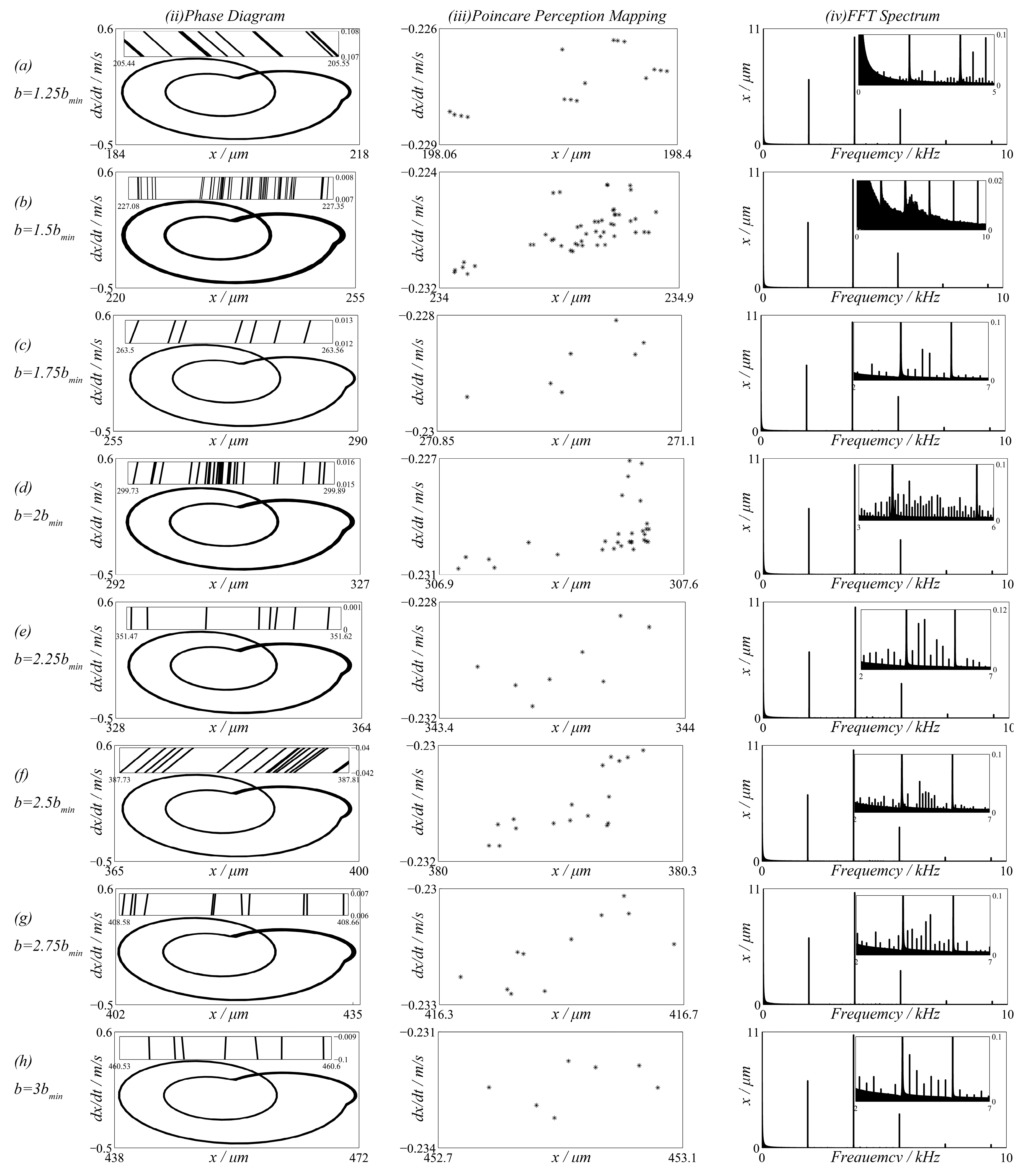
In practical engineering applications, the value range of the backlash is . Here, the research range of the backlash was expanded to to conduct a better study on the influence of backlash on the dynamics. Figure 10 shows the system response in terms of the dynamic transmission error for various backlash values. In the case of , the dynamic motion is non-harmonic-single-periodic as a whole. Partially enlarged views indicated that the system presented a low-frequency vibration, as shown in Figure 10a. The phase diagram had 16 curves, the resulting trace in the Poincare map was concentrated in 16 points, and the enlarged spectrum had peaks at the points of . As a result, the system mainly exhibited non-harmonic-single-periodic vibration and also exhibited 16T-periodic low-frequency vibration with a small amplitude.
As the backlash increased to , the motion was similar to that of where no significant period of low-frequency vibration was presented. As the backlash further increased, the low-frequency vibrations were 7T-periodic in the case of and 30T-periodic in the case of , respectively. According to Figure 10e–h, it was clear that the low-frequency vibrations were 8T-periodic, 16T-periodic, 11T-periodic, and 7T-periodic, respectively.
The dynamic transmission error is a key parameter to evaluate the gear system’s vibration and noise. Available studies have often been concerned with the vibration whose minimum response frequency equals that of the excitation frequency, and those small-amplitude and low-frequency motions have received less attention. According to Figure 9 and Figure 10, it is quite clear that the backlash had a great influence on the small-amplitude and low-frequency vibration, which can be regarded as secondary vibration and can guide us to understanding the mechanism of some special noise.
4. Conclusions
An improved mesh stiffness was proposed by taking the effect of backlash into account. The precise tooth profile equations with backlash were established to generate the gears. The potential energy method was employed to calculate the mesh stiffness. The calculation results indicated that when compared with the case of ignoring backlash, the mesh stiffness had an obvious decrease in the cycle of coming into the mesh to going out of the mesh. Moreover, the rate of decline showed a trend of decreasing first before increasing.
To obtain an accurate stiffness function for numerical analysis, the mesh stiffness rather than the time-varying mesh stiffness was fitted in the form of Fourier series expansion, and the time-varying mesh stiffness was presented in terms of a piecewise function. The proposed fitting mesh used a low order Fourier series to obtain very high accuracy. The stiffness coefficient was also fitted by the Fourier series.
The effects of backlash on dynamic transmission error were investigated, and the numerical results revealed that the gear system primarily performed a non-harmonic-single-periodic motion. The partially enlarged views indicated that the system also exhibited small-amplitude and low-frequency motion. For different cases of backlash, the low-frequency motion sometimes showed excellent periodicity and stability and sometimes showed a non-repetitive and aperiodic situation.
The theory here focused on the impact of backlash on mesh stiffness and dynamic performance and established an indirect relationship between backlash and dynamic transmission error, which is expected in order to understand the mechanism of some unusual noise and to guide the design and manufacture of backlash in the future.
Author Contributions
Conceptualization, methodology, data curation, writing—original draft preparation, visualization, Y.X.; writing—review and editing, funding acquisition, K.H.; investigation, software, validation, F.X., Y.Y. and M.S.; supervision, Z.Z.
Funding
This work was supported by the National Natural Science Foundation of China (51775156) and the Fundamental Research Funds for the Central Universities of China (JZ2018HGTA0206, JZ2018HGBZ0101).
Conflicts of Interest
The authors declare no conflict of interest.
References
- Draft International Standard ISO 6336-1. Calculation of Load Capacity of Spur and Helical Gears; Part I: Basic principles and influence factors; International Organization for Standardization: Geneva, Switzerland, 1990; pp. 87–95. [Google Scholar]
- Walha, L.; Fakhfakh, T.; Haddar, M. Nonlinear dynamics of a two-stage gear system with mesh stiffness fluctuation, bearing flexibility and backlash. Mech. Mach. Theory 2009, 44, 1058–1069. [Google Scholar] [CrossRef]
- Vaishya, M.; Singh, R. Analysis of periodically varying gear mesh systems with Coulomb friction using Floquet theory. J. Sound Vib. 2001, 243, 525–545. [Google Scholar] [CrossRef]
- Yang, J.; Peng, T.; Lim, T.C. An enhanced multi-term harmonic balance solution for nonlinear period-one dynamic motions in right-angle gear pairs. Nonlinear Dyn. 2014, 76, 1237–1252. [Google Scholar] [CrossRef]
- Jiang, H.; Shao, Y.; Mechefske, C.K. Dynamic characteristics of helical gears under sliding friction with spalling defect. Eng. Failure Anal. 2014, 39, 92–107. [Google Scholar] [CrossRef]
- Li, Y.; Ding, K.; He, G.; Lin, H. Vibration mechanisms of spur gear pair in healthy and fault states. Mech. Syst. Signal Process. 2016, 81, 183–201. [Google Scholar] [CrossRef]
- Kuang, J.H.; Yang, Y.T. An estimate of mesh stiffness and load sharing ratio of a spur gear pair. In Proceedings of the ASME Proceedings of International Power Transmission and Gearing Conference, Scottsdale, Arizona, 13–16 September 1992; pp. 1–9. [Google Scholar]
- Parey, A.; El Badaoui, M.; Guillet, F.; Tandon, N. Dynamic modelling of spur gear pair and application of empirical mode decomposition-based statistical analysis for early detection of localized tooth defect. J. Sound Vib. 2006, 294, 547–561. [Google Scholar] [CrossRef]
- Hu, Z.; Tang, J.; Zhong, J.; Chen, S.; Yan, H. Effects of tooth profile modification on dynamic responses of a high speed gear-rotor-bearing system. Mech. Syst. Signal Process. 2016, 76–77, 294–318. [Google Scholar] [CrossRef]
- Tang, J.; Cai, W.; Wang, Z. Meshing stiffness formula of modification gear. J. Central South Univ. 2017, 48, 337–342. [Google Scholar]
- Siyu, C.; Jinyuan, T.; Zehua, H. Comparisons of gear dynamic responses with rectangular mesh stiffness and its approximate form. J. Mech. Sci. Technol. 2015, 29, 3563–3569. [Google Scholar]
- Yang, D.C.H.; Lin, J.Y. Hertzian Damping, Tooth Friction and Bending Elasticity in Gear Impact Dynamics. J. Mech. Des. 1987, 109, 189–196. [Google Scholar] [CrossRef]
- Philippe, S.; Philippe, V.; Olivier, D. Contribution of gear body to tooth deflections—A new bidimensional analytical formula. J. Mech. Des. 2004, 126, 748–752. [Google Scholar]
- Xinhao, T. Dynamic Simulation for System Response of Gearbox Including Localized Gear Faults. Ph.D. Thesis, University of Alberta, Edmonton, AB, Canada, 2004. [Google Scholar]
- Wan, Z.; Cao, H.; Zi, Y.; He, W.; He, Z. An improved time-varying mesh stiffness algorithm and dynamic modeling of gear-rotor system with tooth root crack. Eng. Failure Anal. 2014, 42, 157–177. [Google Scholar] [CrossRef]
- Ma, H.; Zeng, J.; Feng, R.; Pang, X.; Wen, B. An improved analytical method for mesh stiffness calculation of spur gears with tip relief. Mech. Mach. Theory 2016, 98, 64–80. [Google Scholar] [CrossRef]
- Yu, W.; Shao, Y.; Mechefske, C.K. The effects of spur gear tooth spatial crack propagation on gear mesh stiffness. Eng. Failure Anal. 2015, 54, 103–119. [Google Scholar] [CrossRef]
- Li, Z.; Ma, H.; Feng, M.; Zhu, Y.; Wen, B. Meshing characteristics of spur gear pair under different crack types. Eng. Failure Anal. 2017, 80, 123–140. [Google Scholar] [CrossRef]
- Chen, Z.; Zhang, J.; Zhai, W.; Wang, Y.; Liu, J. Improved analytical methods for calculation of gear tooth fillet-foundation stiffness with tooth root crack. Eng. Failure Anal. 2017, 82, 72–81. [Google Scholar] [CrossRef]
- Ma, H.; Feng, M.; Li, Z.; Feng, R.; Wen, B. Time-varying mesh characteristics of a spur gear pair considering the tip-fillet and friction. Meccanica 2017, 52, 1695–1709. [Google Scholar] [CrossRef]
- Lei, Y.; Liu, Z.; Wang, D.; Yang, X.; Liu, H.; Lin, J. A probability distribution model of tooth pits for evaluating time-varying mesh stiffness of pitting gears. Mech. Syst. Signal Process. 2018, 106, 355–366. [Google Scholar] [CrossRef]
- Ma, H.; Yang, J.; Song, R.; Zhang, S.; Wen, B. Effects of Tip Relief on Vibration Responses of a Geared Rotor System. Proc. Inst. Mech. Eng. Part C J. Mech. Eng. Sci. 2014, 228, 1132–1154. [Google Scholar] [CrossRef]
- Guo, Y.; Parker, R.G. Analytical determination of back-side contact gear mesh stiffness. Mech. Mach. Theory 2014, 78, 263–271. [Google Scholar] [CrossRef]
- Yogesh, P.; Anand, P. Simulation of crack propagation in spur gear tooth for different gear parameter and its influence on mesh stiffness. Eng. Failure Anal. 2013, 30, 124–137. [Google Scholar]
- Chen, Q.; Ma, Y.; Huang, S.; Zhai, H. Research on gears’ dynamic performance influenced by gear backlash based on fractal theory. Appl. Surface Sci. 2014, 313, 325–332. [Google Scholar] [CrossRef]
- Zhixiong, L.; Zeng, P. Nonlinear dynamic response of a multi-degree of freedom gear system dynamic model coupled with tooth surface characters: A case study on coal cutters. Nonlinear Dyn. 2015, 84, 1–16. [Google Scholar]
- Saghafi, A.; Farshidianfar, A. An analytical study of controlling chaotic dynamics in a spur gear system. Mech. Mach. Theory 2016, 96, 179–191. [Google Scholar] [CrossRef]
- Xianzeng, L.; Yuhu, Y.; Jun, Z. Investigation on coupling effects between surface wear and dynamics in a spur gear system. Tribol. Int. 2016, 101, 383–394. [Google Scholar]
- Yun, Y.J.; Byeongil, K. Effect and feasibility analysis of the smoothening functions for clearance-type nonlinearity in a practical driveline system. Nonlinear Dyn. 2016, 85, 1651–1664. [Google Scholar] [CrossRef]
- Xiangfeng, G.; Lingyun, Z.; Dailin, C. Bifurcation and chaos analysis of spur gear pair in two-parameter plane. Nonlinear Dyn. 2015, 79, 2225–2235. [Google Scholar]
- Wang, J.; Howard, I. The torsional stiffness of involute spur gears. Proc. Inst. Mech. Eng. Part C: J. Mech. Eng. Sci. 2004, 218, 131–142. [Google Scholar] [CrossRef]
- Suit, Z. A rotary model for spur gear dynamics. J. Mech. Trans. Autom. Des. 1985, 107, 529–535. [Google Scholar]
- Farshidianfar, A.; Saghafi, A. Global bifurcation and chaos analysis in nonlinear vibration of spur gear systems. Nonlinear Dyn. 2014, 75, 783–806. [Google Scholar] [CrossRef]
- Wang, J.; Yang, J.; Li, Q. Quasi-static analysis of the nonlinear behavior of a railway vehicle gear system considering time-varying and stochastic excitation. Nonlinear Dyn. 2018, 93, 463–485. [Google Scholar] [CrossRef]
Figure 1.
The principle of the generating method: (a) involute; (b) transition curve.

Figure 2.
The geometric model of the gear profile.

Figure 3.
The single-tooth-pair mesh stiffness.
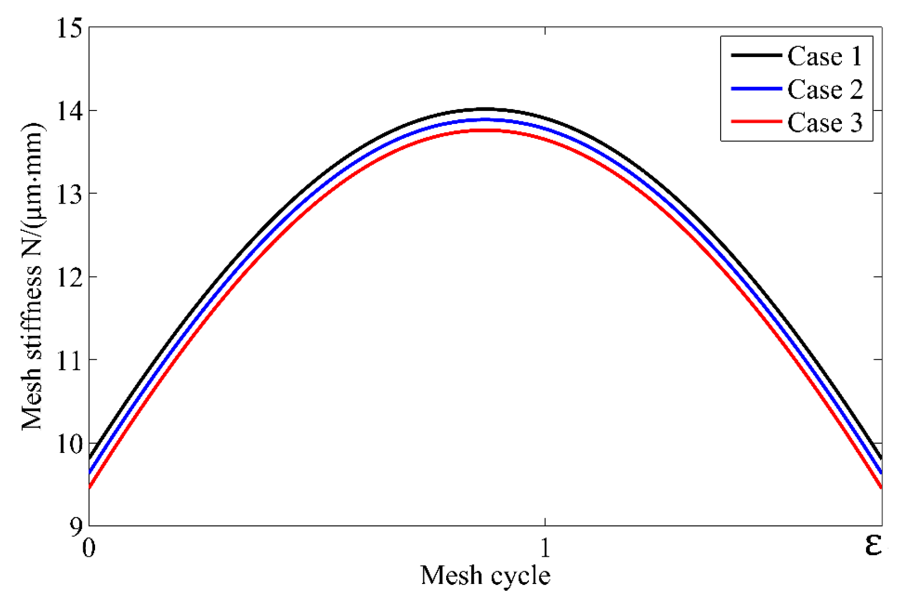
Figure 4.
The time-varying mesh stiffness.
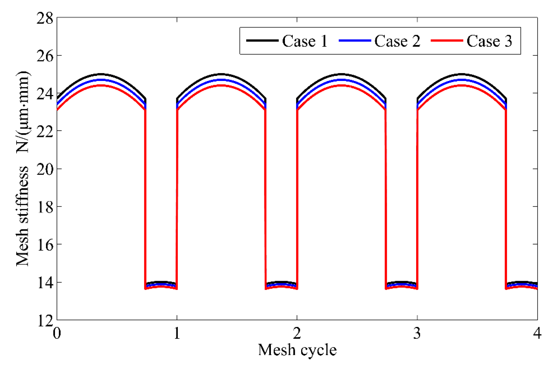
Figure 5.
for the different values of backlash.
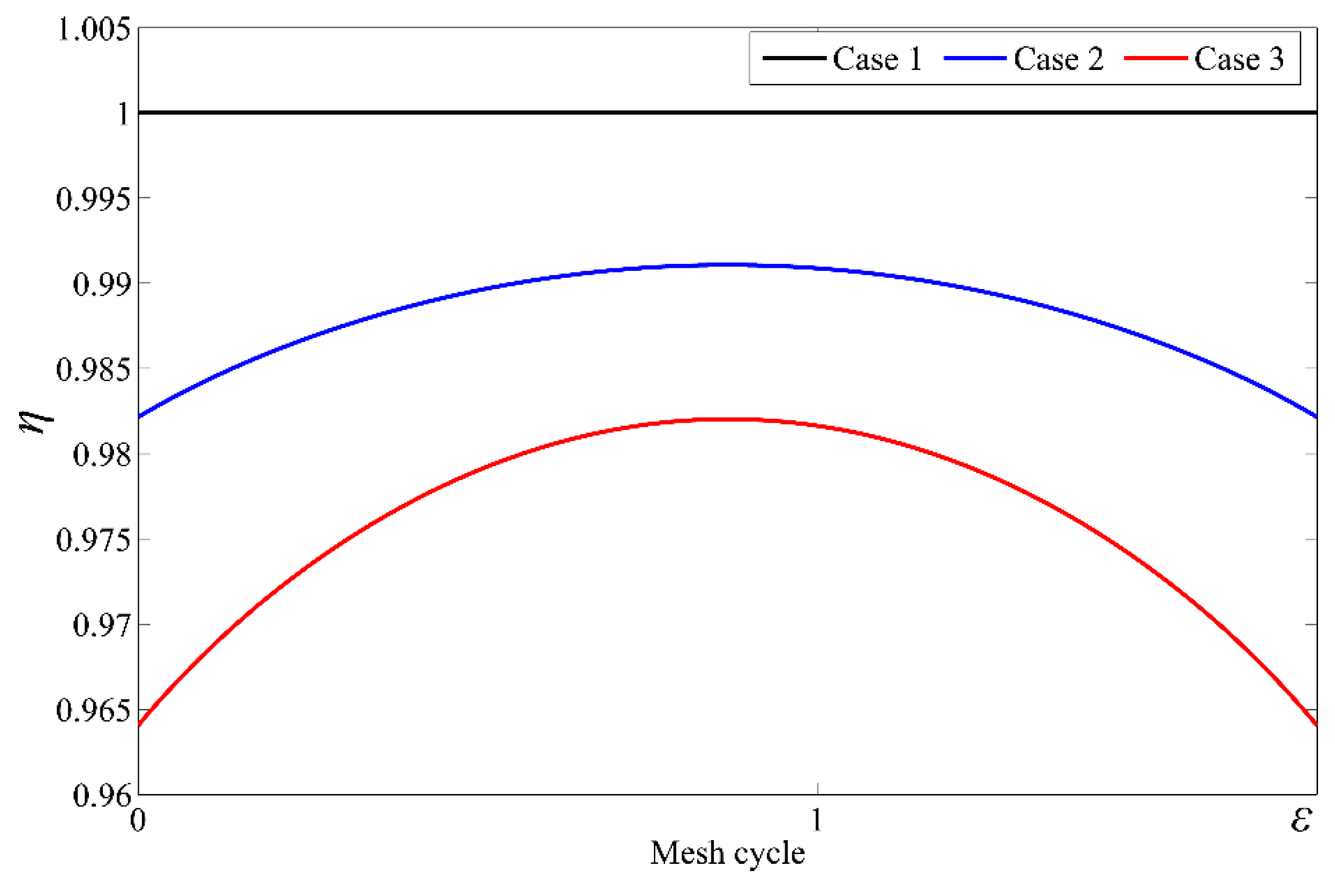
Figure 6.
The single-tooth-pair mesh stiffness: (a) Comparison of calculated stiffness and fitted stiffness. (b) Relative error curve.
Figure 6.
The single-tooth-pair mesh stiffness: (a) Comparison of calculated stiffness and fitted stiffness. (b) Relative error curve.

Figure 7.
A snapshot of the contact pattern (at t = 0) of a spur gear pair.

Figure 8.
The non-linear dynamic model.

Figure 9.
The system response in terms of the dynamic transmission error for .
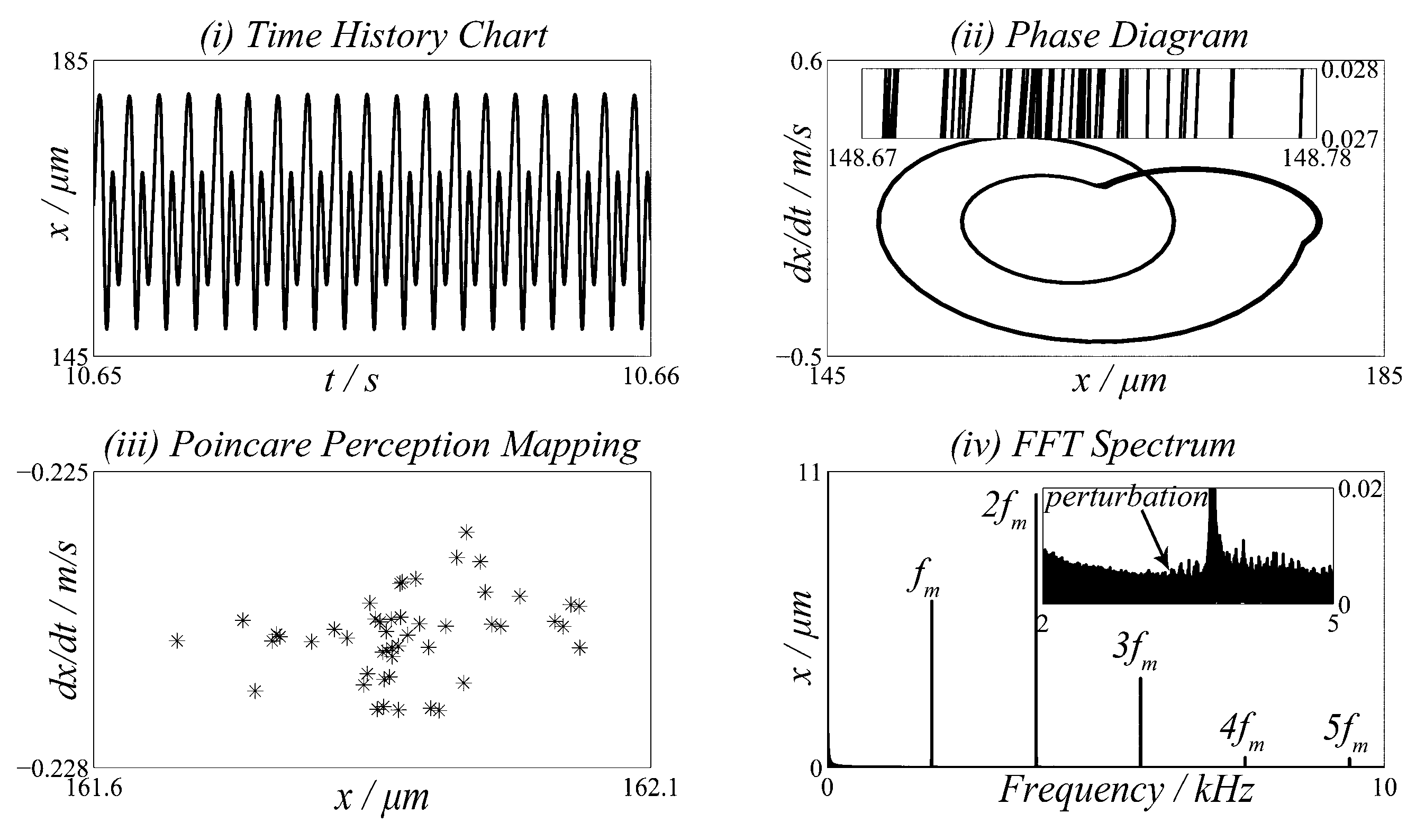
Figure 10.
The system response in terms of the dynamic transmission error of various backlash. (a) ; (b) ; (c) ; (d) ; (e) ; (f) ;(g) ; (h) .
Figure 10.
The system response in terms of the dynamic transmission error of various backlash. (a) ; (b) ; (c) ; (d) ; (e) ; (f) ;(g) ; (h) .


Table 1.
The values of the coefficients of Equation (12).
| –5.574 10−5 | –1.9986 10−3 | –2.3015 10−4 | 4.7702 10−3 | 0.0271 | 6.8045 | |
| 60.111 10−5 | 28.100 10−3 | –83.431 10−4 | –9.9256 10−3 | 0.1624 | 0.9086 | |
| –50.952 10−5 | 185.50 10−3 | 0.0538 10−4 | 53.3 10−3 | 0.2895 | 0.9236 | |
| –6.2042 10−5 | 9.0889 10−3 | –4.0964 10−4 | 7.8297 10−3 | –0.1472 | 0.6904 |
Table 2.
The parameters of the example gear pair.
| Properties | Symbol | Value (Unit) |
|---|---|---|
| Young’s modulus | E | |
| Poisson’s ratio | 0.3 | |
| Pressure angle | ||
| Width of teeth | ||
| Number of teeth | 45/45 | |
| Module | 3 | |
| Radius of the inner hub | 25 | |
| Addendum coefficient | 1 | |
| Clearance coefficient | 0.25 | |
| Contact ratio | 1.7358 |
Table 3.
The fitting parameters for the example gear pair.
© 2019 by the authors. Licensee MDPI, Basel, Switzerland. This article is an open access article distributed under the terms and conditions of the Creative Commons Attribution (CC BY) license (http://creativecommons.org/licenses/by/4.0/).
Share and Cite
MDPI and ACS Style
Xiong, Y.; Huang, K.; Xu, F.; Yi, Y.; Sang, M.; Zhai, H. Research on the Influence of Backlash on Mesh Stiffness and the Nonlinear Dynamics of Spur Gears. Appl. Sci. 2019, 9, 1029. https://doi.org/10.3390/app9051029
AMA Style
Xiong Y, Huang K, Xu F, Yi Y, Sang M, Zhai H. Research on the Influence of Backlash on Mesh Stiffness and the Nonlinear Dynamics of Spur Gears. Applied Sciences. 2019; 9(5):1029. https://doi.org/10.3390/app9051029
Chicago/Turabian StyleXiong, Yangshou, Kang Huang, Fengwei Xu, Yong Yi, Meng Sang, and Hua Zhai. 2019. "Research on the Influence of Backlash on Mesh Stiffness and the Nonlinear Dynamics of Spur Gears" Applied Sciences 9, no. 5: 1029. https://doi.org/10.3390/app9051029
Note that from the first issue of 2016, this journal uses article numbers instead of page numbers. See further details here.