Consensus Algorithms Based Multi-Robot Formation Control under Noise and Time Delay Conditions

Abstract

In recent years, the formation control of multi-mobile robots has been widely investigated by researchers. With increasing numbers of robots in the formation, distributed formation control has become the development trend of multi-mobile robot formation control, and the consensus problem is the most basic problem in the distributed multi-mobile robot control algorithm. Therefore, it is very important to analyze the consensus of multi-mobile robot systems. There are already mature and sophisticated strategies solving the consensus problem in ideal environments. However, in practical applications, uncertain factors like communication noise, communication delay and measurement errors will still lead to many problems in multi-robot formation control. In this paper, the consensus problem of second-order multi-robot systems with multiple time delays and noises is analyzed. The characteristic equation of the system is transformed into a quadratic polynomial of pure imaginary eigenvalues using the frequency domain analysis method, and then the critical stability state of the maximum time delay under noisy conditions is obtained. When all robot delays are less than the maximum time delay, the system can be stabilized and achieve consensus. Compared with the traditional Lyapunov method, this algorithm has lower conservativeness, and it is easier to extend the results to higher-order multi-robot systems. Finally, the results are verified by numerical simulation using MATLAB/Simulink. At the same time, a multi-mobile robot platform is built, and the proposed algorithm is applied to an actual multi-robot system. The experimental results show that the proposed algorithm is finally able to achieve the consensus of the second-order multi-robot system under delay and noise interference.

1. Introduction

In recent years, with the continuous development of computer science, complex network theory and control theory, autonomous mobile robots have received more and more attention [1]. Compared to single mobile robots, multi-mobile robot systems have better stability, higher fault tolerance and higher work efficiency. As a result, they have better application prospects and higher research value in the fields of reconnaissance, patrol, rescue and environmental survey. Formation control of multi-mobile robots is the basis of multi-mobile robot systems, and has become a hotspot in the field of robotics [2].

As part of the design process of multi-robot formation control algorithm, many problems need to be considered, including robot model, external environmental interference, sensor measurement noise, algorithm control precision, and the controllability of different formations [3]. The existing formation control algorithms for multi-robots mainly include the leader-follower algorithm [4], the behavior-based algorithm [5], the graph theory-based method [6], the virtual structure method [7], and the artificial potential field method. The leader-follower algorithm has flexible motion strategy and scalability, but the algorithm cannot form stable and reliable feedback between the follower and the leader. Therefore, the control error of the follower will increase with interference from the environment. In particular, when the leader fails, it can cause the entire multi-robot system to crash. The behavior-based algorithm can effectively reduce the complexity of the entire formation control algorithm, but it has higher requirements in terms of sensor sensing ability and communication ability between robots, and cannot accurately quantify the behavior of robots during operation. Thus, it is difficult to guarantee the system’s robustness using the behavior-based algorithm. The virtual structure method is convenient for designing the formation behavior of multi-robot systems, while due to the constraints of rigid structures, it lacks flexibility with respect to obstacle avoidance and formation transformation. The artificial potential field algorithm has a simple structure and can effectively avoid collisions and obstacles, but it is susceptible to interference when maintaining the formation, and it is difficult to perform precise formation control. Moreover, the potential energy function needs to be reset if the formation transformation is performed, leading to a lack of flexibility.

In view of the shortcomings of the traditional formation control algorithm, considering the increase in the number of robots in the multi-robot system and the continuous improvement of the data processing capability of a single robot, the distributed multi-robot control algorithm has attracted the attention of researchers. The distributed multi-robot system can make full use of the data processing resources of the robot and share the pressure of the central processing machine, which has great advantages in terms of flexibility and fault tolerance [8,9]. In addition, solving the consensus problem is the core of the distributed multi-robot control algorithm [10]. There are already mature and sophisticated strategies for solving the consensus problem in ideal environments [11,12]. However, in practical applications, uncertain factors like communication noise, communication delay and measurement error will still lead to many problems in multi-robot formation control. Some algorithms have considered some practical problems. Reference [13] studied the conditions of the system reaching consensus under uniform delay, when the communication structures of second-order multi-robot systems were a directed graph with spanning tree or a strongly connected graph, respectively. However, that paper does not consider the noise condition or consensus under different delay conditions. Reference [14] studied the consensus problem of second-order multi-robot systems under noisy conditions. A control protocol based on distributed sampling data was proposed to achieve system consensus, but the delay condition was not taken into account in the algorithm. Reference [15] studied the consensus of second-order multi-robot systems under non-uniform and multi-time delays using the frequency domain analysis method. Compared with the Lyapunov method, it has lower conservativeness, and the results were extended to higher-order multi-robot systems. However, it did not take noise into consideration, which is unavoidable in practical environments. Reference [16] studied the consensus of second-order multi-robot systems under uniform time delay and noise environments, and designed different control protocols for different types of noise, thus achieving the consensus of the system. These algorithms provide some basic solutions to the second-order system consensus problem, but the problems encountered by multi-robots in practical applications are far more varied than these. On the basis of these algorithms, this paper performs a more in-depth analysis, especially considering the consensus of the second-order system in which there are many different time delays and multiplicative noises in the system, laying the foundations for a formation control algorithm for second-order multi-robot systems that can be truly implemented in real robot systems.

In summary, this paper analyzes the consensus problem of second-order multi-robot systems under various delay and noise conditions. The system character equations are transformed into quadratic polynomials of pure imaginary eigenvalues based on frequency domain analysis, and then solved. Finally, its critical steady state is obtained and verified using Matlab numerical simulation. Compared with existing algorithms, this algorithm has lower conservativeness, and it is easier to extend the results to higher-order multi-robot systems. Since the omnidirectional mobile robot is a fully driven robot, and the horizontal and vertical directions can be separately controlled, it can be constructed as two one-dimensional second-order multi-robot systems. Therefore, experiments were carried out on a multi-omnidirectional mobile robot platform built in the laboratory using the proposed algorithm [17,18], which verifies the effectiveness of the proposed algorithm.

2. Pre-Preparation and Problem Description

2.1. Graph Theory

$G=\{V,E\}$ represents the communication topology between robots, in which each robot represents a node. $V$ is a set of nodes. $E$ is a set of edges, representing the connection state between robots. The topology map is represented by a Laplacian matrix, which is $L=D-A$. $D$ is the degree matrix, which represents how many nodes are adjacent to each node. $A=[a_{ij}]$ is the adjacent matrix and $i,j\in V$. $N_i$ represents all sets of nodes adjacent to the $i$ node. If node $j$ is adjacent to node $i$, then $a_{ij}>0$. If $a_{ij}=a_{ji}$ for any $i,j\in V$, the graph is an undirected graph; otherwise, it is a directed graph. If there is a directed path on any two nodes in the graph, the directed graph $G$ is strongly connected. If there is a directed path to a node in the graph to any other node, then the directed graph $G$ contains a spanning tree. If the undirected graph $G$ is strongly connected, it is called a connected graph. When the undirected graph $G$ is a connected graph, its Laplacian $L$ matrix contains a zero root, and the other eigenvalues are positive real numbers. When a directed graph $G$ contains a spanning tree, its Laplacian $L$ matrix contains a zero root, and the rest eigenvalue’s real part are positive.

2.2. Problem Description

Suppose the system consists of n omnidirectional robots. The dynamic characteristics of the omnidirectional robot in the x direction are:

$$\{\begin{array}{l}{\dot{x}}_i(t)=v_i(t)\\ {\dot{v}}_i(t)=u_i(t)\end{array}$$

(1)

where $x_i(t)$ is position, $v_i(t)$ is velocity and $u_i(t)$ is input control. If any i robot and j robot in the multi-robot system satisfy the identities as follows:

$$\underset{t\to +\infty }{\lim }[x_i(t)-x_j(t)]=0$$

(2)

$$\underset{t\to +\infty }{\lim }[v_i(t)-v_j(t)]=0$$

(3)

then the multi-robot system (1) has achieved consensus under the control protocol $u_i(t)$ Let the state vector of the i robot be ${\delta }_i(t)={\left[x_i(t),v_i(t)\right]}^T$, then the multi-robot system state vector is $S(t)=\left[{\delta }_1(t),{\delta }_2(t),{\delta }_3(t),\dots ,{\delta }_n(t)\right]$. Rewrite system (1) as:

$$\dot{S}(t)=\Psi S(t)$$

(4)

where $\Psi =I\otimes A-L\otimes B$, $A=\left[\begin{array}{cc}0& 1\\ 0& 0\end{array}\right]$, $B=\left[\begin{array}{cc}0& 0\\ k_1& k_2\end{array}\right]$, $\otimes$ is Kronecker. When ideally without noise and delay, the control protocol designed in [13] is as follows:

$$u_i(t)={\displaystyle \sum _{j\in N_i}{a}_{ij}\left\{k_1[x_i(t)-x_j(t)]+k_2[v_i(t)-v_j(t)]\right\}}$$

(5)

where $a_{ij}>0$ is the topology weight of the communication between robot i and robot j, $k_1$ is the position scale factor that needs to be designed, $k_2$ is the velocity scale factor that needs to be designed. Lemmas 1 and 2 give the conditions that the coefficient matrix $\Psi$ of control protocol (5) must satisfy when the communication topology of system (4) is undirected graph and directed graph, respectively.

Lemma 1.

When the communication topology of multi-robot system (4) is connected graph, the coefficient matrix$\Psi$has a double zero root, and the real part of other eigenvalues is negative.

Proof. 

Let there be an orthogonal matrix $Q$, such that:

$$Q^{T}LQ=diag\{0,{\lambda }_2,{\lambda }_3,\dots ,{\lambda }_n\}$$

(6)

where $0,{\lambda }_2,{\lambda }_3,\dots ,{\lambda }_n$ is the eigenvalue of the Laplacian matrix $L$, and ${\lambda }_i$ > 0 ($i$ = 2, 3, …, n). Formula (7) is obtained from Formula (6):

$${(Q\otimes I_2)}^T\psi (Q\otimes I_2)=diag\{A,A-{\lambda }_{2}B,A-{\lambda }_{3}B,\dots ,A-{\lambda }_{n}B\}$$

(7)

The determinant of Formula (7) is obtained:

$$\left|diag\{A,A-{\lambda }_{2}B,A-{\lambda }_{3}B,\dots ,A-{\lambda }_{n}B\}\right|=s^2{\displaystyle \prod _2^n{s}^2+{\lambda }_i{k}_{2}s+{\lambda }_i{k}_1}=0$$

(8)

Because there is $s^2$ in Formula (8), there must be a double zero root in the eigenvalue. By solving polynomial equation $s^2+{\lambda }_i{k}_{2}s+{\lambda }_i{k}_1=0$, we can get:

$$s_1=\frac{-{\lambda }_i{k}_2+\sqrt{{({\lambda }_i{k}_2)}^2-4{\lambda }_i{k}_1}}{2}$$

$$s_2=\frac{-{\lambda }_i{k}_2-\sqrt{{({\lambda }_i{k}_2)}^2-4{\lambda }_i{k}_1}}{2}$$

Based on this analysis, when ${({\lambda }_i{k}_2)}^2$ > $4{\lambda }_i{k}_1$, obviously $-{\lambda }_i{k}_2\pm \sqrt{{({\lambda }_i{k}_2)}^2-4{\lambda }_i{k}_1}$ < 0, so the eigenvalues $s_1$ and $s_2$ are negative. When ${({\lambda }_i{k}_2)}^2$ < $4{\lambda }_i{k}_1$, because ${\lambda }_i{k}_2$ > 0, so $-{\lambda }_i{k}_2$ < 0, the eigenvalues $s_1$ and $s_2$ have negative real parts. Lemma 1 is proved.  □

Lemma 2.

When the communication topology of multi-robot system (4) is directed graph and contains spanning tree,$k_1\in (0,k_0{k}_2^2)$the coefficient matrix$\Psi$has a double zero root, and the real part of other eigenvalues is negative. Where$k_0=\underset{\Vert {\lambda }_i\Vert \ne 0}{\min }\left\{\frac{{\Vert {\lambda }_i\Vert }^2\mathrm{real}({\lambda }_i)}{\mathrm{imag}({\lambda }_i)}\right\}$.

Proof. 

The characteristic determinant of system (4) is obtained by Formula (8), assuming that there are polynomial equations:

$$s^2+s(a+bj)+k(a+bj)=0$$

(9)

where $a$ > 0, $k,a,b\in R$. Let $s=jw$:

$$-w^2-bw+ka+(aw+kb)j=0$$

(10)

Solving Formula (10), we can get:

$$\{\begin{array}{l}-w^2-bw+ka=0\\ aw+kb=0\end{array}$$

(11)

Thus, solved:

$$\{\begin{array}{l}{k}_1=0\\ k_2=\frac{a(a^2+b^2)}{b^2}\end{array}$$

(12)

Document [13] proves that when $0<k<\frac{a(a^2+b^2)}{b^2}$, the roots of Formula (9) are all on the left open half plane. Formula (8) is modified according to Formula (9):

$$s^2{\displaystyle \prod _2^n{s}^2+{\lambda }_i{k}_{2}s+{\lambda }_i\frac{k_1}{k_2}}{k}_2=0$$

(13)

The analysis shows that when $k_0=\underset{\Vert {\lambda }_i\Vert \ne 0}{\min }\left\{\frac{{\Vert {\lambda }_i\Vert }^2\mathrm{real}({\lambda }_i)}{\mathrm{imag}({\lambda }_i)}\right\}$, $k_1\in (0,k_0{k}_2^2)$, the coefficient matrix $\Psi$ has a double zero root, and the real part of other eigenvalues is negative. Lemma 2 is proved.  □

3. Consensus Analysis of Multi-Robot with Various Delays and Noise Conditions

In the previous section, we analyzed the conditions under which second-order systems achieve consensus in an ideal environment. However, in real environments, due to noise interference and communication differences between different robotic hardware, the above control protocols need to be improved. Assuming that there are D kinds of different delays in the system, the multi-agent system (4) can be changed to:

$$\dot{S}(t)=(I\otimes A)·S(t)-{\displaystyle \sum _{\mathrm{d}=1}^D(L_d\otimes B)·\zeta (t)·S(t-{\tau }_d)}$$

(14)

where $\zeta (t)$ is the communication noise or measurement noise between robots, ${\tau }_{ij}$ is the transmission delay, which represents the time taken by $i$ robot to receive and process information transmitted by $j$ robot, $L_d$ is the Laplacian matrix corresponding to the sub-topological graph of the robot node when the delay is ${\tau }_d$, and ${\displaystyle \sum _{\mathrm{d}=1}^D{L}_d}=L$.

Theorem 1.

If system (14) is a connected graph, the system can achieve consensus when the system delay${\tau }_d$is less than${\tau }_{\max }$under the action of noise$\zeta (t)$. Among them:

$$\{\begin{array}{l}{\tau }_{\max }=\left[\arctan \left(\frac{k_2}{k_1}{w}_{\max }\right)\right]/w_{\max }\\ w_{\max }=\sqrt{\frac{{\lambda }_{\max }^2{k}_2^2{\zeta }^2(t)+\zeta (t)\sqrt{{\zeta }^2(t){({\lambda }_{\max }^2{k}_2^2)}^2+4{\lambda }_{\max }^2{k}_1^2}}{2}}\end{array}$$

(15)

Proof. 

Using the frequency domain analysis method for analysis, the Laplace transform of Equation (14) can be obtained:

$$S(s)=(s{{\rm I}}_{2n}-({{\rm I}}_n\otimes A)+{\displaystyle \sum _{\mathrm{d}=1}^D(L_d\otimes B)\zeta (t)e^{-{\tau }_{d}s}}){}^{-1}S(0)$$

(16)

Let $G_{\tau }(s)=s{{\rm I}}_{2n}-({{\rm I}}_n\otimes A)+{\displaystyle \sum _{\mathrm{d}=1}^D(L_d\otimes B)\zeta (t)e^{-{\tau }_{d}s}}$, so the eigenvalues of the determinant $\left|G_{\tau }(s)\right|$ are the eigenvalues of the system. Lemma 1 proves that multi-robot system (4) achieves the conditions of consensus. According to Lemma 1, how can the eigenvalues of system (14) be kept in the negative half-plane under the interference of time delay $\tau$ and noise $\zeta (t)$ relative to the system (4)? Because the measurement noise and communication noise are uncertainties in real environments, it is impossible to carry out accurate quantitative analysis. Therefore, only when the system delay $\tau$ increases to a value under the action of noise $\zeta (t)$ does a non-zero eigenvalue of the system appear on the virtual axis for the first time, while the time delay $\tau$ is the critical value for the system to maintain stability.

Assuming that the eigenvalue of the system is on the imaginary axis, let $s=jw$ be the eigenvalue; then $\alpha ={\alpha }_1\otimes {[1,0]}^T+{\alpha }_2\otimes {[0,1]}^T$ is the eigenvector corresponding to the eigenvalue, and if $\Vert \alpha \Vert =1$, ${\alpha }_1,{\alpha }_2\in {ℂ}^n$, then:

$$\left[jw{{\rm I}}_{2n}-({{\rm I}}_n\otimes A)+{\displaystyle \sum _{\mathrm{d}=1}^D(L_d\otimes B)\zeta (t)e^{-jw{\tau }_d}}\right]\alpha =0$$

(17)

The imaginary eigenvalues of the system appear in pairs in conjugate form. This paper only analyzes the case where $w$ > 0. Formula (17) left multiplied by ${\alpha }^H$ is:

$${\alpha }^H\left[jw{{\rm I}}_{2n}-({{\rm I}}_n\otimes A)+{\displaystyle \sum _{\mathrm{d}=1}^D(L_d\otimes B)\zeta (t)e^{-jw{\tau }_d}}\right]\alpha =0$$

(18)

Because each line of the left matrix of Formula (17) is zero, so $jw{\alpha }_1={\alpha }_2$, and substituting it into Formula (18):

$${\displaystyle \sum _{\mathrm{d}=1}^D{\beta }_d\zeta (t)e^{-jw{\tau }_d}}=\frac{w^2}{k_1+jw{k}_2}$$

(19)

where ${\beta }_d=\frac{{\alpha }^H(L_d\otimes I_2)\alpha }{{\alpha }^H\alpha }$. Replace A with B in Formula (19):

$$F(w)={\displaystyle \sum _{\mathrm{d}=1}^D{\beta }_d\zeta (t)e^{jw{\tau }_d}}=\frac{w^2}{k_1-jw{k}_2}$$

(20)

Take module operation on both sides of the upper equal sign:

$$\Vert F(w)\Vert =\Vert {\displaystyle \sum _{\mathrm{d}=1}^D{\beta }_d\zeta (t)e^{-jw{\tau }_d}}\Vert <\Vert {\displaystyle \sum _{\mathrm{d}=1}^D{\beta }_d\zeta (t)}\Vert =\frac{{\alpha }^H(L\otimes I_2)\alpha }{{\alpha }^H\alpha }\zeta (t)\le {\lambda }_{\max }\zeta (t)$$

(21)

Let $w_{\max }=\sqrt{\frac{{\lambda }_{\max }^2{k}_2^2{\zeta }^2(t)+\zeta (t)\sqrt{{\zeta }^2(t){({\lambda }_{\max }^2{k}_2^2)}^2+4{\lambda }_{\max }^2{k}_1^2}}{2}}$ get $w\le w_{\max }$, upper formula establishment. From Formula (20):

$$\theta (w)=\mathrm{argz}[F(w)]=\arctan (\frac{k_2}{k_1}w)$$

(22)

where $\theta (w)\in [0,2\pi )$. Let $\tau (w)=\frac{\theta (w)}{w},a=\frac{k_2}{k_1}$, deriving for $\tau (w)$, we can obtain:

$$M_1(w)=\frac{d\tau (w)}{dw}=\frac{1}{w^2}{M}_2(w)=\frac{1}{w^2}\left[\frac{aw}{a^2{w}^2+1}-\arctan (aw)\right]$$

(23)

Deriving for $M_2(w)$ we can obtain:

$$\frac{d{M}_2(w)}{dw}=-\frac{2a^3{w}^2}{{(a^2{w}^2+1)}^2}<0$$

(24)

$M_2(w)$ is decreasing, so when $w>0$, $M_2(w)<M_2(0)=0$, so $M_1(w)$ < 0; that is, $\tau (w)$ is also decreasing. So $\tau (w)\ge \tau (w_{\max })={\tau }_{\max }$. When ${\tau }_d<{\tau }_{\max }$, when ${\tau }_d<{\tau }_{\max }$, we can get:

$$\tau (w)=\frac{\theta (w)}{w}=\frac{\arg z\left({\displaystyle \sum _{\mathrm{d}=1}^D{\beta }_d\zeta (t)e^{jw{\tau }_d}}\right)}{w}\le \frac{\max [w{\tau }_d]}{w}<\frac{w{\tau }_{\max }}{w}<{\tau }_{\max }$$

(25)

That is to say, it contradicts $\tau (w)\ge \tau (w_{\max })$. Therefore, when ${\tau }_d<{\tau }_{\max }$, the eigenvalues of the system can be maintained in the left half plane, and the consensus of system (14) can be achieved. Theorem 1 is proved.  □

Theorem 2.

If system (14) is a directed graph and there is a spanning tree, the system can achieve consensus when the system delay${\tau }_d$is smaller than the${\tau }_{\max }$under the action of noise$\zeta (t)$, and$k_1\in (0,k_0{k}_2^2)$. Among them:

$$\{\begin{array}{l}{\tau }_{\max }=\underset{\Vert {\lambda }_i\Vert \ne 0}{\min }\left[\left[\arctan \left(\frac{k_2}{k_1}{w}_i\right)-\arg z({\lambda }_i)\right]/w_i\right]\\ w_i=\sqrt{\frac{{\lambda }_i^2{k}_2^2{\zeta }^2(t)+\zeta (t)\sqrt{{\zeta }^2(t){({\lambda }_i^2{k}_2^2)}^2+4{\lambda }_i^2{k}_1^2}}{2}}\end{array}$$

(26)

where$\arg z({\lambda }_i)\in (-\frac{\pi }{2},\frac{\pi }{2})$.

Proof. 

Lemma 2 proved that, when the communication topology of multi-robot system (4) is directed graph and contains spanning tree, $k_1\in (0,k_0{k}_2^2)$, the coefficient matrix $\Psi$ has a double zero root, and the real part of the other eigenvalues is negative. The same analysis is performed using the frequency domain analysis method. Similar to the proof of Theorem 1, only when the system delay $\tau$ increases to the value under the action of noise $\zeta (t)$ does a non-zero eigenvalue of the system first appear on the imaginary axis, while the delay $\tau$ is the critical value for the system to maintain stability. Take modulo operation on Formula (20):

$$\Vert F(w)\Vert =\Vert \frac{w^2}{k_1-jw{k}_2}\Vert$$

(27)

Let $w$ be a function of $\Vert F(w)\Vert$; then the above formula can be written as follows:

$$w=\sqrt{\frac{{\Vert F(w)\Vert }^2{k}_2^2+\sqrt{{({\Vert F(w)\Vert }^2{k}_2^2)}^2+4{\Vert F(w)\Vert }^2{k}_1^2}}{2}}$$

(28)

Then we can get that $w$ is an incremental function about $\Vert F(w)\Vert$. From Formula (20):

$$\{\begin{array}{l}\mathrm{argz}[F(w)]=\arctan (\frac{k_2}{k_1}w)\\ \mathrm{argz}[F(w)]\le \arg z({\displaystyle \sum _{\mathrm{d}=1}^D{\beta }_d})+\max (w{\tau }_m)\end{array}$$

(29)

So:

$$\arctan (\frac{k_2}{k_1}w)-\arg z({\displaystyle \sum _{\mathrm{d}=1}^D{\beta }_d})\le \max (w{\tau }_m)$$

(30)

Because ${\beta }_d=\frac{{\alpha }^H(L_d\otimes I_2)\alpha }{{\alpha }^H\alpha }$, so ${\displaystyle \sum _{\mathrm{d}=1}^D{\beta }_d}={\lambda }_i$,where ${\lambda }_i$ is the non-zero eigenvalue of Laplace matrix $L$. So $\Vert F(w)\Vert \le \Vert \zeta (t){\lambda }_i\Vert$. Because $w$ is an incremental function about $\Vert F(w)\Vert$, so:

$$w(\Vert F(w)\Vert )\le w(\Vert \zeta (t){\lambda }_i\Vert )=w_i=\sqrt{\frac{{\lambda }_i^2{k}_2^2{\zeta }^2(t)+\zeta (t)\sqrt{{\zeta }^2(t){({\lambda }_i^2{k}_2^2)}^2+4{\lambda }_i^2{k}_1^2}}{2}}$$

(31)

When ${\tau }_d<{\tau }_{\max }$, we can get:

$$\begin{array}{cc}\hfill \max (w{\tau }_d)<w_i{\tau }_{\max }& =\min \left[\left[\arctan (\frac{k_2}{k_1}{w}_i)-\arg z({\displaystyle \sum _{\mathrm{d}=1}^D{\beta }_d})\right]/w_i\right]w_i\hfill \\ & \le \arctan (\frac{k_2}{k_1}w)-\arg z({\displaystyle \sum _{\mathrm{d}=1}^D{\beta }_d})\hfill \end{array}$$

(32)

We can find that this contradicts Formula (30), so when ${\tau }_d<{\tau }_{\max }$, the eigenvalue of the system can be maintained in the left half plane, and the consensus of system (14) can be achieved. Theorem 2 is proved. □

4. Simulation Verification

In this section, two sets of Matlab/Simulink numerical simulation experiments are carried out to verify the consensus of the system described in Theorems 1 and 2 when the communication topology is undirected graph and directed graph under the conditions of noise and various delays.

Experiment 1.

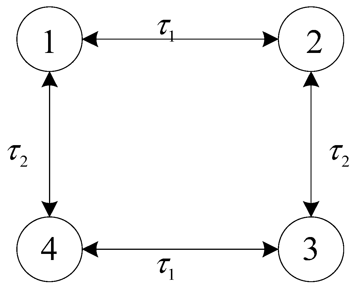
Let system (14) consist of four robots whose communication topology is shown in Figure 1.

As can be seen from Figure 1, the time delay between robots 1 and 2 is ${\tau }_1$, between robot 2 and robot 3 it is ${\tau }_2$, between robot 3 and robot 4 it is ${\tau }_1$, between robot 4 and robot 1 it is ${\tau }_2$. If the adjacent communication weight $a_{ij}$ is 1, then the Laplace matrix $L$ is:

$$L=\left(\begin{array}{cccc}2& -1& & -1\\ -1& 2& -1& \\ & -1& 2& -1\\ -1& & -1& 2\end{array}\right)$$

(33)

We can get ${\lambda }_{\max }=4$. Assume that the communication noise or measurement noise is white noise with a maximum amplitude of two. According to Theorem 1, ${\tau }_{\max }=0.226$.

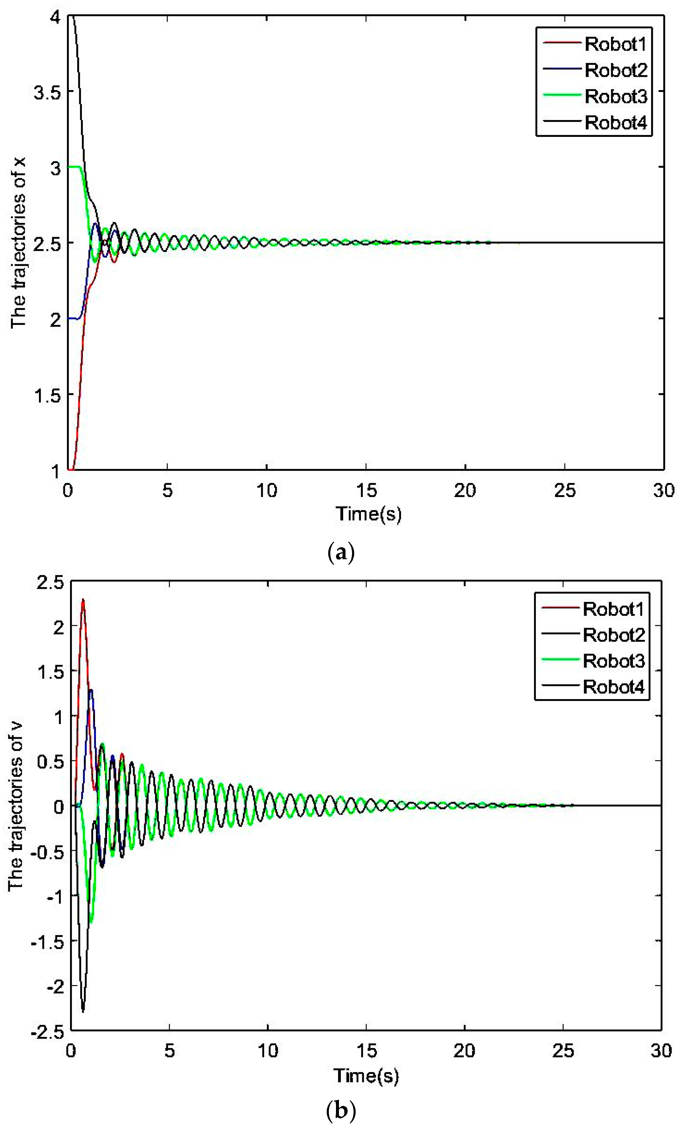
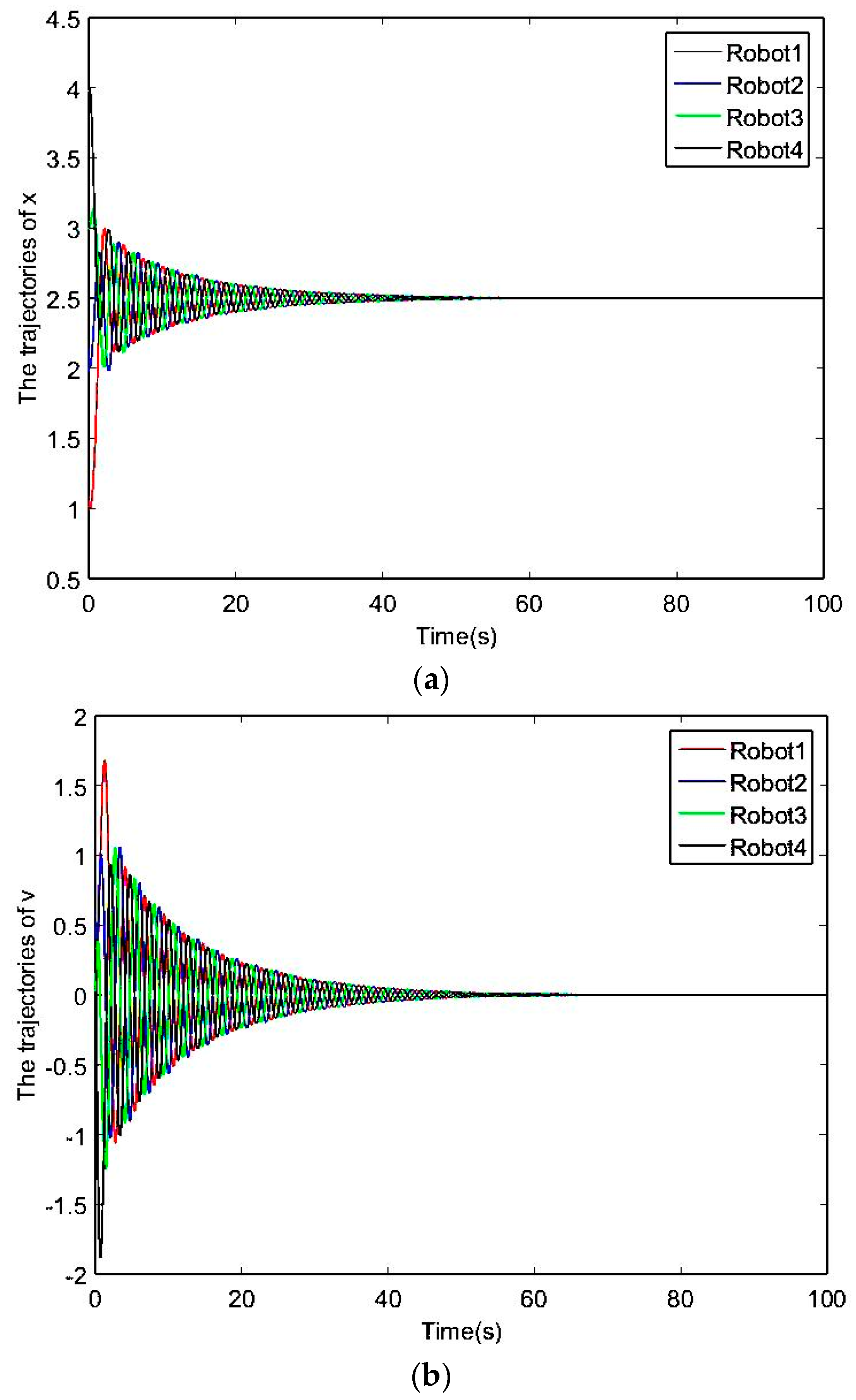
In the first group of Experiment 1, set ${\tau }_1=0.21$, ${\tau }_2=0.22$, and the initial posture is assumed to be (1,0), (2,0), (3,0), (4,0). The simulation results are shown in Figure 2.

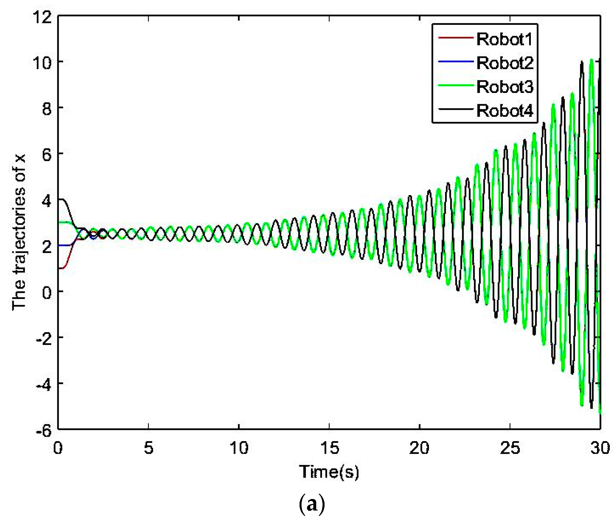
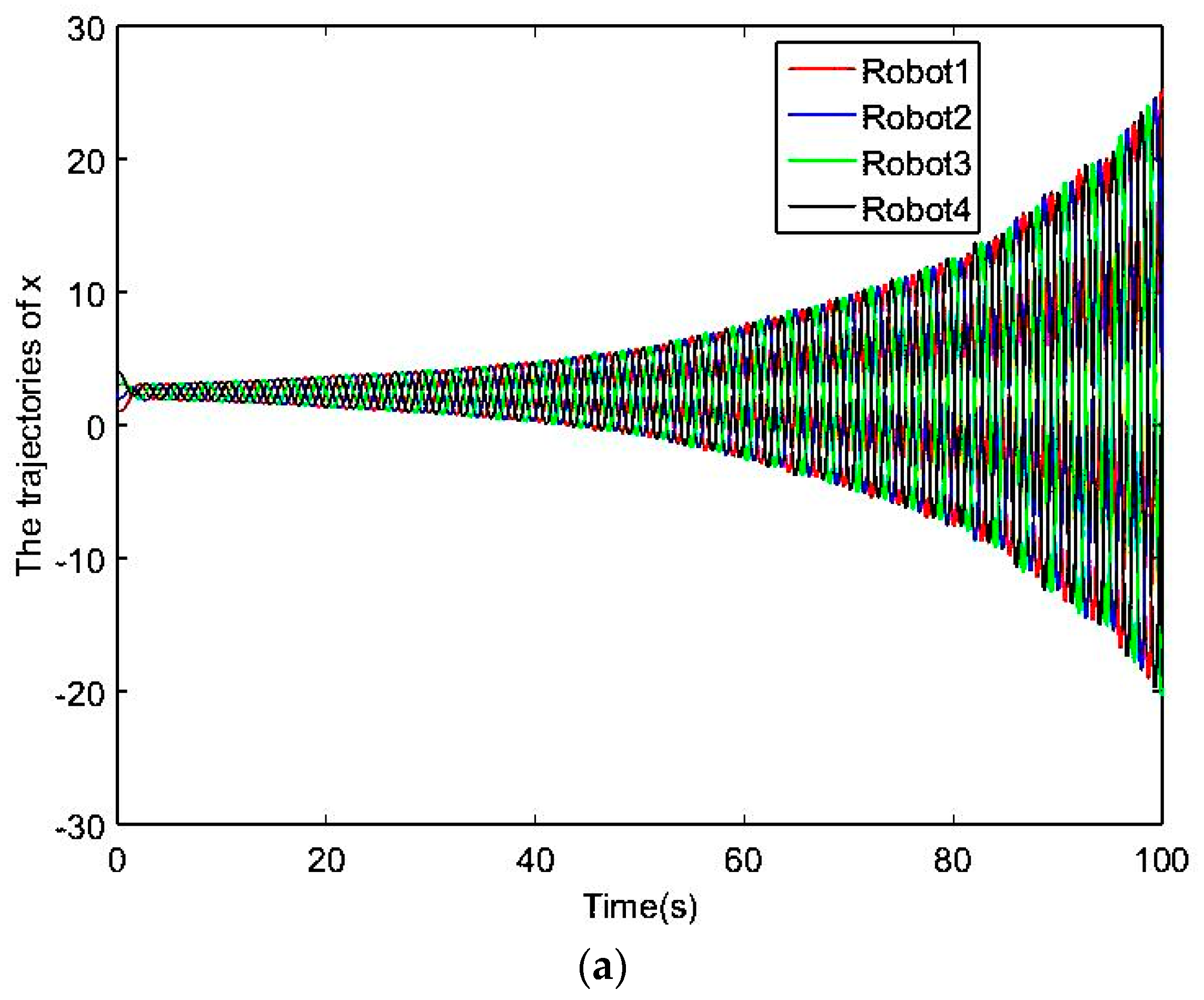
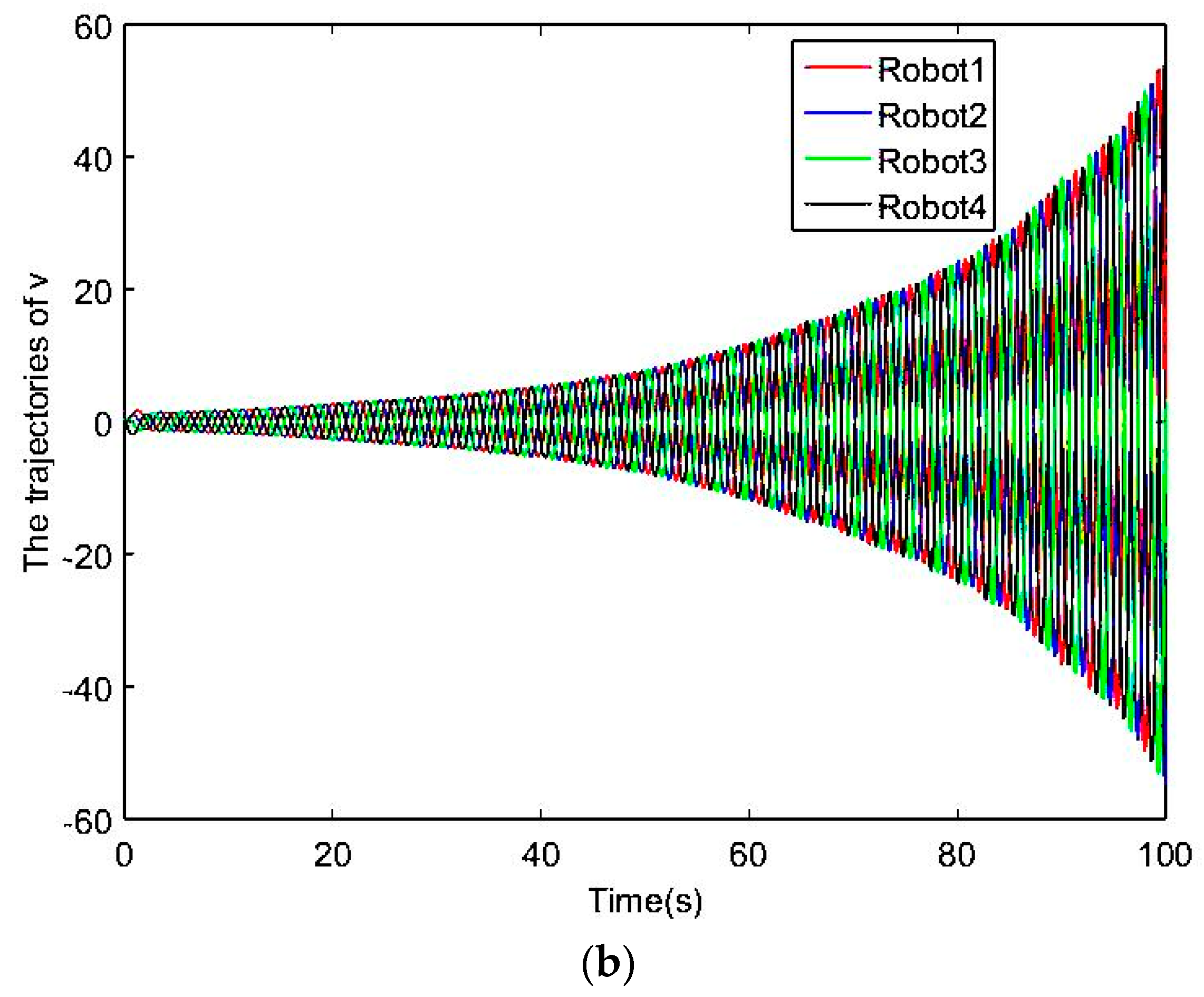
To verify Theorem 1 and compare with the first group of experiments, in the second group of experiments, set ${\tau }_1=0.23$, ${\tau }_2=0.24$ under the same conditions. The simulation results are shown in Figure 3.

According to Experiment 1, system (14) satisfying lemma 1 can achieve consensus when all ${\tau }_d$ are less than ${\tau }_{\max }$, and the system will diverge when all ${\tau }_d$ are greater than ${\tau }_{\max }$, which cannot achieve consensus; thus Theorem 1 is verified.

Experiment 2.

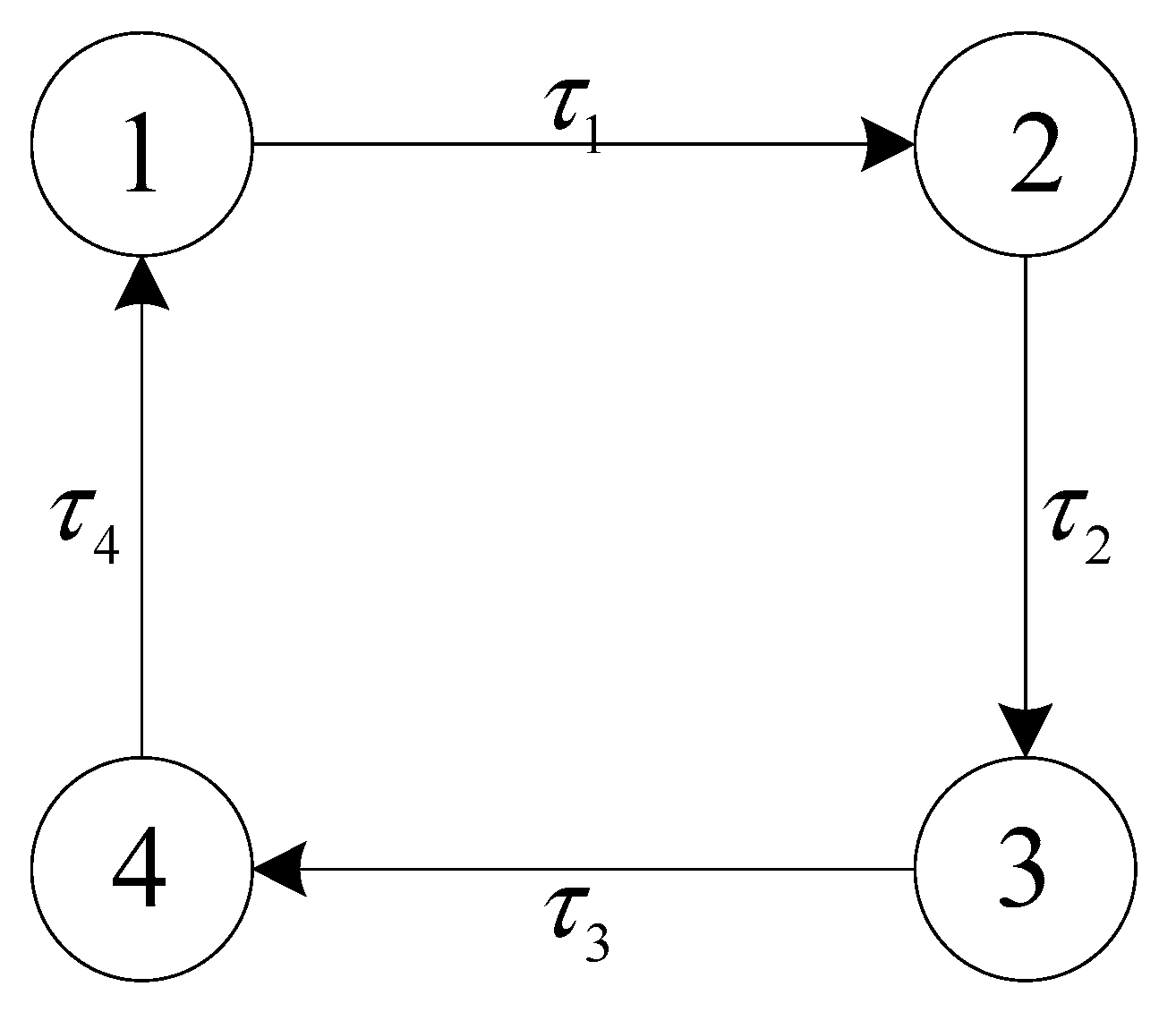
Let system (14) consist of four robots whose communication topology is shown in Figure 4.

The time delay from Robot 1 to Robot 2 is ${\tau }_1$, from Robot 2 to Robot 3 it is ${\tau }_2$, from Robot 3 to Robot 4 it is ${\tau }_3$, from Robot 4 to Robot 1 it is ${\tau }_4$. If the adjacent communication weight $a_{ij}$ is 1, then the Laplace matrix $L$ is:

$$L=\left(\begin{array}{cccc}2& & -1& \\ -1& 1& & -1\\ & -1& 2& \\ -1& & -1& 1\end{array}\right)$$

(34)

Then $k_0=\underset{\Vert {\lambda }_i\Vert \ne 0}{\min }\left\{\frac{{\Vert {\lambda }_i\Vert }^2\mathrm{real}({\lambda }_i)}{\mathrm{imag}({\lambda }_i)}\right\}=\frac{5\times 2}{1}=10$, so $k_1\in (0,10k_2^2)$. Assume that the communication noise or measurement noise is white noise with a maximum amplitude of two. Set $k_1=1$, $k_2=1$, according to Theorem 2, ${\tau }_{\max }=0.137$.

In the first group of experiment 2, set ${\tau }_1=0.13$, ${\tau }_2=0.12$, ${\tau }_3=0.11$, ${\tau }_4=0.1$, and the initial posture is assumed to be (1,0), (2,0), (3,0), (4,0). The simulation results are shown in Figure 5.

To verify Theorem 2 and compare with the first group of experiments, in the second group of experiments, set ${\tau }_1=0.14$, ${\tau }_2=0.141$, ${\tau }_3=0.142$, ${\tau }_4=0.143$ under the same conditions. The simulation results are shown in Figure 6.

According to experiment 2, system (14) satisfying Lemma 2 can achieve consensus when all ${\tau }_d$ are less than ${\tau }_{\max }$, and the system will diverge when all ${\tau }_d$ are greater than ${\tau }_{\max }$, which cannot achieve consensus; thus Theorem 2 is verified.

5. Physical Experiment Verification

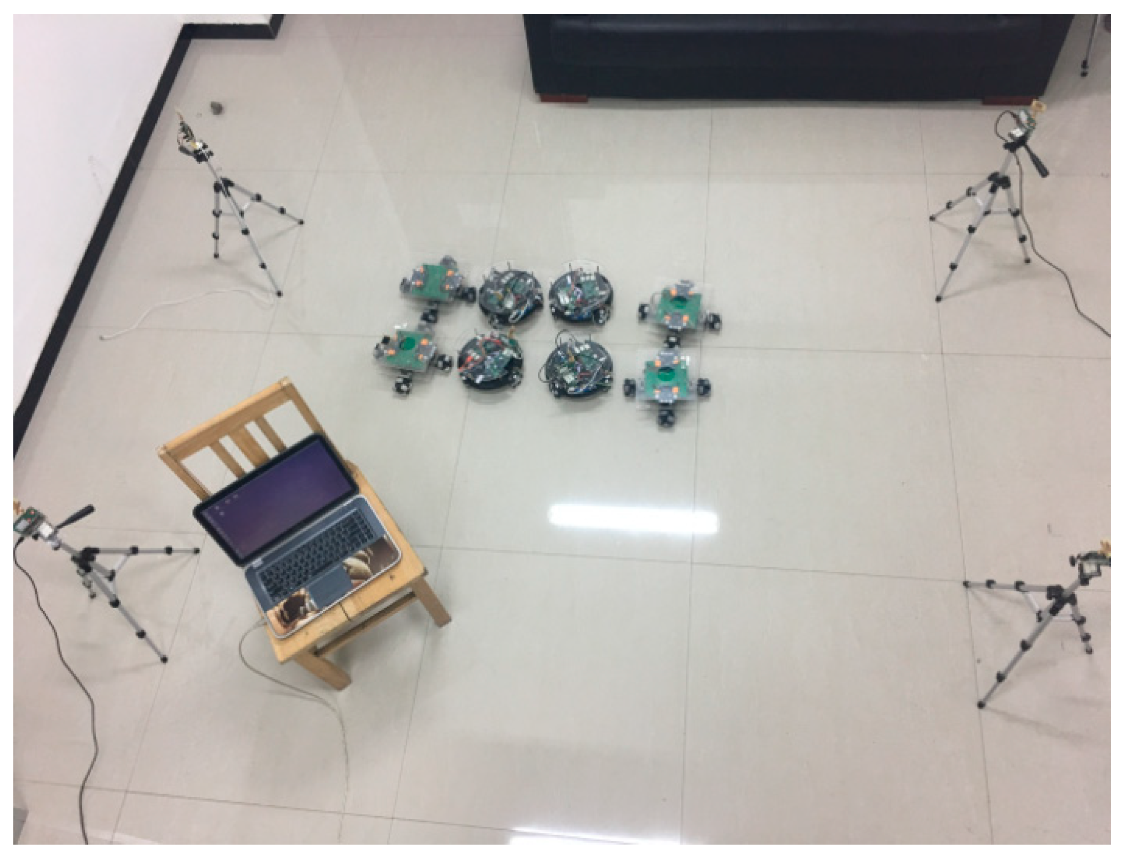
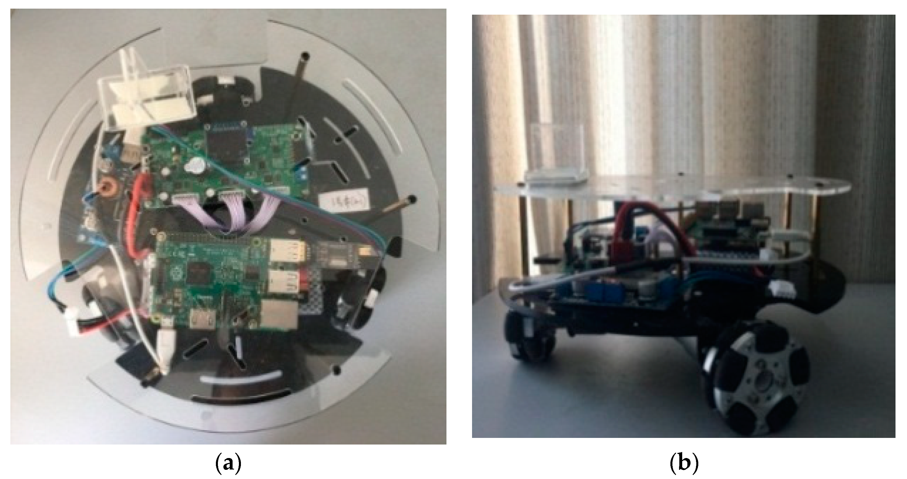
To verify the proposed formation control algorithm, we did the experiment based on a pre-constructed multi-mobile robot research platform built by our laboratory, which was constructed with a self-designed three-wheeled omnidirectional robot carrying an UWB (Ultra-Wide Band) ranging module. The system is shown in Figure 7, the omnidirectional robot is shown in Figure 8, and the performance parameters are shown in

Table 1. Omnidirectional robot parameters.

Parameter Name	Value
weight	1.5 Kg
diameter	235 mm
Maximum linear velocity	1.2 m/s
Maximum angular velocity	6.6 rad/s
Battery capacity	2800 mah
No-load Maximum Standby Time	2 h
Maximum Load Weight	3 Kg

. Because the consensus of the second-order system is analyzed in the theoretical analysis part, the speed and position are consistent, and while the omnidirectional robot is a fully driven robot, the horizontal and vertical directions can be controlled separately. Because the velocity control in a given direction is a second-order system, therefore, multi-omni-directional mobile robots can be decomposed into two one-dimensional second-order multi-robot systems. Therefore, omni-directional robots are used to verify the proposed algorithm. In the experiment, it is possible to determine whether the algorithm is valid based on whether the speed and the position of the robot after final stabilization are consistent. In the data acquisition part, the external positioning data of the robot are collected by the UWB positioning system built by myself, and the speed of the robot itself is collected by the encoder on the wheel of the robot and transmitted to the central processing computer via Wi-Fi for processing. The ranging error between the UWB ranging modules used in the experiment is 7 cm. Experiments were carried out in an indoor environment with length × width of 4 m × 5 m in order to verify the effectiveness of the proposed algorithm.

It should be pointed out that when the proposed algorithm is applied to a practical multi-robot system, it is necessary to first determine the maximum communication delay between robots and the maximum amplitude of the noise environment, and then design $k_1$ and $k_2$ based on this. At the same time, it should be noted that this experiment mainly focuses on verifying whether the system can achieve consensus under the control law. The collision avoidance behavior of the multi-robot system is not the emphasis in this research. Therefore, the collision avoidance algorithm program is written in the bottom control program of the robot in this experiment. When the robot is about to collide, the formation algorithm program will be interrupted, and the collision avoidance behavior will be executed. When a safe distance between the robots has been reached, the formation algorithm program will continue to be executed [17,18].

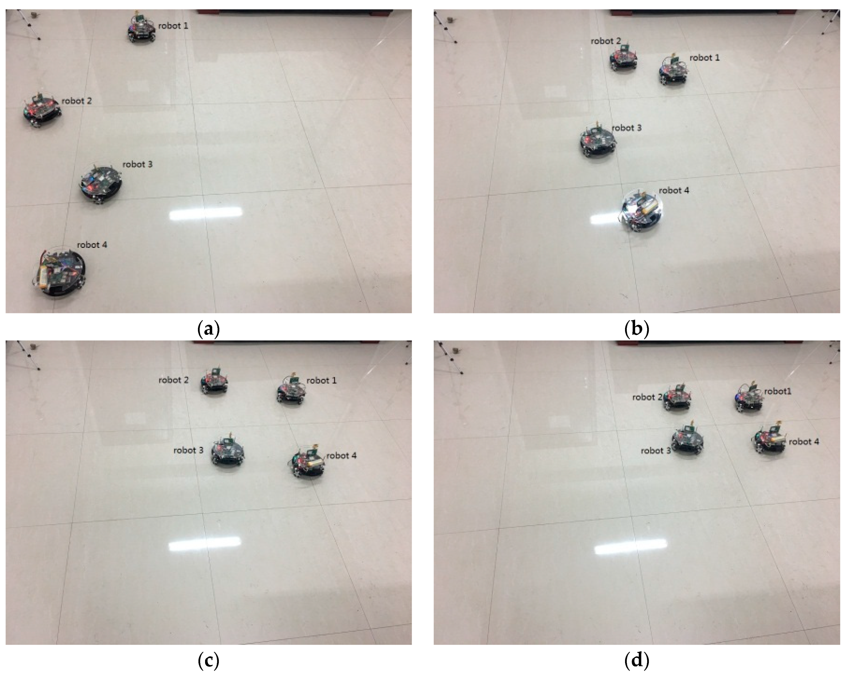
The communication topology used in the experiment is shown in Figure 4. The adjacent communication weight $a_{ij}$ is 1, so $k_1\in (0,10k_2^2)$. The central processor logs on each robot remotely through SSH, and obtains the communication delay between two robots whose communication weight A is not zero by PING command. The time delay between robots in the actual communication environment is time-varying, so take its maximum delay. We get ${\tau }_{a1}=0.56s$, ${\tau }_{a2}=0.043s$, ${\tau }_{a3}=0.047s$, ${\tau }_{a4}=0.061s$. The time taken for each robot to receive data and process them is ${\tau }_{b1}=0.021s$, ${\tau }_{b2}=0.02s$, ${\tau }_{b3}=0.021s$, ${\tau }_{b4}=0.021s$. Therefore, the time delay between robots is ${\tau }_1=0.077s$, ${\tau }_2=0.063s$, ${\tau }_3=0.068s$, ${\tau }_4=0.082s$. Because this experiment is being performed in a laboratory environment, it is assumed that the communication noise is white noise with a maximum amplitude of 2. According to Formula (26) and the moving speed of omnidirectional robot, set $k_1=1$, $k_2=1.4$. Four omnidirectional robots were placed in arbitrary positions, (0.83,2.20,0), (0.35,1.74,0), (0.67,0.88,0), (0.56,0.48,0), respectively. In the practicality experiment, the robot cannot converge to one point, so Formula (2) is changed to:

$$\underset{t\to +\infty }{\lim }[x_i(t)-x_j(t)-F_p]=0$$

(35)

where $F_p$ is the formation parameters and p = 1, 2, …, n. Since the system only installs a UWB ranging sensor to provide positioning for the robot, the robot will perform pose determination before the experiment starts, and the robot’s body coordinate system will be consistent with the global coordinate system. The experimental results are shown in Figure 9. The experimental video address can be found in reference [19].

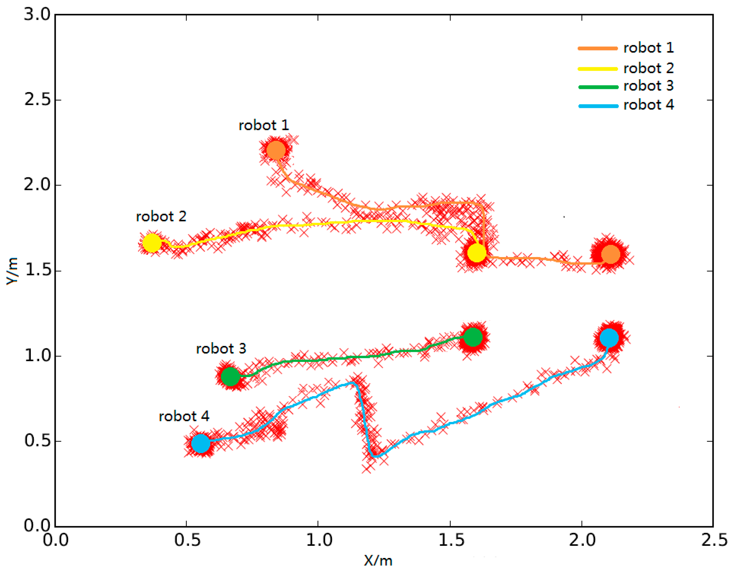
The experimental data collected by the UWB positioning system are shown in Figure 10.

The experiments show that the multi-robot system can eventually achieve consensus and form a formation in a variety of time-delay and noise environments, which verifies the effectiveness of the proposed algorithm.

6. Conclusions

Aiming at the consensus of multi-mobile robots under uncertain conditions such as communication delay, communication noise and measurement noise, we used the frequency domain analysis method, transformed the characteristic equation into the quadratic polynomial of the pure imaginary eigenvalue, and then obtained the conditions for achieving consensus under various time delay and noise conditions for a second-order multi-robot system. That is, when the time delays of all robots are less than the maximum time delays, the system can achieve consensus. In this paper, based on two aspects of system communication topology—directed graph and undirected graph—the results were verified by numerical simulation using MATLAB/Simulink, verifying the correctness of the theoretical derivation of the proposed algorithm. Finally, a multi-robot research platform was built, and formation control experiments were carried out in a real laboratory environment. The experimental results showed that the proposed algorithm could effectively make the second-order multi-mobile robot systems consistent. This paper only analyzes the consensus problem of second-order systems, while most existing multi-mobile robot systems are higher-order systems. Therefore, the consensus analysis of higher-order systems under noise and time delay conditions will be the focus of our next research.

References

- Nelson, E.; Corah, M.; Michael, N. Environment model adaptation for mobile robot exploration. Auton. Robots 2018, 42, 257–272. [Google Scholar] [CrossRef]
- Alonso-Mora, J.; Montijano, E.; Nägeli, T.; Hilliges, O.; Schwager, M.; Rus, D. Distributed multi-robot formation control in dynamic environments. Auton. Robots 2018, 1–22. [Google Scholar] [CrossRef]
- Yang, X.; Hua, C.C.; Yan, J.; Guan, X.P. Adaptive Formation Control of Cooperative Teleoperators With Intermittent Communications. IEEE Trans. Cybern. 2018, 3. [Google Scholar] [CrossRef] [PubMed]
- Trinh, M.H.; Zhao, S.; Sun, Z.; Zelazo, D.; Anderson, B.D.O.; Ahn, H.-S. Bearing-Based Formation Control of A Group of Agents with Leader-First Follower Structure. IEEE Trans. Autom. Control 2018. [Google Scholar] [CrossRef]
- Galceran, E.; Cunningham, A.G.; Eustice, R.M.; Olson, E. Multipolicy decision-making for autonomous driving via changepoint-based behavior prediction: Theory and experiment. Auton. Robots 2017, 41, 1367–1382. [Google Scholar] [CrossRef]
- Li, X.; Xie, L. Dynamic Formation Control Over Directed Networks Using Graphical Laplacian Approach. IEEE Trans. Autom. Control 2018, 56, 21–35. [Google Scholar] [CrossRef]
- Pan, W.W.; Jiang, D.P.; Pang, Y.J.; Li, Y.M.; Zhang, Q. A multi-AUV formation algorithm combining artificial potential field and virtual structure. Acta Armamentarii 2017, 38, 326–334. [Google Scholar] [CrossRef]
- Xin, L.; Zhu, D. An Adaptive SOM Neural Network Method to Distributed Formation Control of a Group of AUVs. IEEE Trans. Ind. Electron. 2018. [Google Scholar] [CrossRef]
- Liu, Z.; Wang, L.; Wang, J.; Dong, D.; Hu, X. Distributed sampled-data control of nonholonomic multi-robot systems with proximity networks. Automatica 2017, 77, 170–179. [Google Scholar] [CrossRef] [Green Version]
- Porfiri, M.; Roberson, D.G.; Stilwell, D.J. Tracking and formation control of multiple autonomous agents: A two-level consensus approach. Automatica 2007, 43, 1318–1328. [Google Scholar] [CrossRef]
- Du, H.; Zhu, W.; Wen, G.; Duan, Z.; Lü, J. Distributed Formation Control of Multiple Quadrotor Aircraft Based on Nonsmooth Consensus Algorithms. IEEE Trans. Cybern. 2019, 49, 342–353. [Google Scholar] [CrossRef] [PubMed]
- Li, S.; Er, M.J.; Zhang, J. Distributed Adaptive Fuzzy Control for Output Consensus of Heterogeneous Stochastic Nonlinear Multiagent Systems. IEEE Trans. Fuzzy Syst. 2018, 26, 1138–1152. [Google Scholar] [CrossRef]
- Lin, P.; Jia, Y.; Du, J.; Yuan, S. Distributed Consensus Control for Second-Order Agents with Fixed Topology and Time-Delay. In Proceedings of the 26th Chinese Control Conference, Zhangjiajie, China, 26–31 July 2007; pp. 577–581. [Google Scholar] [CrossRef]
- Cheng, L.; Wang, Y.; Hou, Z.G.; Tian, M.; Cao, Z. Sampled-data based average consensus of second-order integral multi-agent systems: Switching topologies and communication noises. Automatica 2013, 49, 1458–1464. [Google Scholar] [CrossRef]
- Mengji, S.; Kaiyu, Q. Distributed Control for Multiagent Consensus Motions with Nonuniform Time Delays. Math. Probl. Eng. 2016, 1–10. [Google Scholar] [CrossRef]
- Wang, B.; Tian, Y.P. Consensus of second-order discrete-time multi-agent systems with relative-state-dependent noises. Int. J. Robust Nonlinear Control 2017, 27, 4591–4606. [Google Scholar] [CrossRef]
- Lv, Q.; Wei, H.; Lin, H.; Zhang, Y. Design and implementation of multi robot research platform based on UWB. In Proceedings of the 2017 29th Chinese Control and Decision Conference (CCDC), Chongqing, China, 28–30 May 2017; pp. 7246–7251. [Google Scholar] [CrossRef]
- Wei, H.; Lv, Q.; Wang, G.-S.; Lin, H.; Liang, B. Trajectory tracking control for heterogeneous mobile robots based on improved UWB ranging. J. Beijing Univ. Aeronaut. Astronaut. 2018, 44, 1461–1471. [Google Scholar] [CrossRef]
- Available online: http://i.youku.com/i/UNDUxODcyNDI0NA==/videos?spm=a2hzp.8244740.0.0 (accessed on 3 January 2019).
Figure 1.
Experiment 1 system communication topology.
Figure 2.
Experiment 1 Group 1 simulation results; is position, is velocity. (a) Trajectory of x changing with time; (b) Trajectory of v changing with time.
Figure 3.
Experiment 1 Group 2 simulation results; is position, is velocity. (a) Trajectory of x changing with time; (b) Trajectory of v changing with time.
Figure 4.
Experiment 2 system communication topology.
Figure 5.
Experiment 2 Group 1 simulation results; is position, is velocity. (a) Trajectory of x changing with time; (b) Trajectory of v changing with time.
Figure 6.
Experiment 2 Group 2 simulation results; is position, is velocity. (a) Trajectory of x changing with time; (b) Trajectory of v changing with time.
Figure 7.
Multi-robot research platform.
Figure 8.
Omnidirectional robots. (a) Top view; (b) Side view.
Figure 9.
Experiment process screenshots. (a) T = 0 s; (b) T = 15 s; (c) T = 25 s; (d) T = 30 s.
Figure 10.
Experiment 1 data of UWB positioning system.