Impact of Texture Information on Crop Classification with Machine Learning and UAV Images


Department of Geoinformatic Engineering, Inha University, Incheon 22212, Korea
*
Author to whom correspondence should be addressed.
Appl. Sci. 2019, 9(4), 643; https://doi.org/10.3390/app9040643
Submission received: 28 January 2019
/
Revised: 12 February 2019
/
Accepted: 12 February 2019
/
Published: 14 February 2019
(This article belongs to the Special Issue Machine Learning Techniques Applied to Geoscience Information System and Remote Sensing)
Abstract
:Unmanned aerial vehicle (UAV) images that can provide thematic information at much higher spatial and temporal resolutions than satellite images have great potential in crop classification. Due to the ultra-high spatial resolution of UAV images, spatial contextual information such as texture is often used for crop classification. From a data availability viewpoint, it is not always possible to acquire time-series UAV images due to limited accessibility to the study area. Thus, it is necessary to improve classification performance for situations when a single or minimum number of UAV images are available for crop classification. In this study, we investigate the potential of gray-level co-occurrence matrix (GLCM)-based texture information for crop classification with time-series UAV images and machine learning classifiers including random forest and support vector machine. In particular, the impact of combining texture and spectral information on the classification performance is evaluated for cases that use only one UAV image or multi-temporal images as input. A case study of crop classification in Anbandegi of Korea was conducted for the above comparisons. The best classification accuracy was achieved when multi-temporal UAV images which can fully account for the growth cycles of crops were combined with GLCM-based texture features. However, the impact of the utilization of texture information was not significant. In contrast, when one August UAV image was used for crop classification, the utilization of texture information significantly affected the classification performance. Classification using texture features extracted from GLCM with larger kernel size significantly improved classification accuracy, an improvement of 7.72%p in overall accuracy for the support vector machine classifier, compared with classification based solely on spectral information. These results indicate the usefulness of texture information for classification of ultra-high-spatial-resolution UAV images, particularly when acquisition of time-series UAV images is difficult and only one UAV image is used for crop classification.
1. Introduction
Agricultural environments are known to be sensitive to abnormal weather conditions and climatic disasters such as drought and flood [1,2], thus rendering essential systematic monitoring of crop conditions and crop yield forecasting [3,4]. Remote sensing technology received attention in the agriculture community due to its ability to provide periodic and regional information for crop monitoring and thematic mapping [5,6].
Crop type maps derived from classification of remote sensing images are important resources for crop yield estimation and forecasting. Since any error in the crop type maps affects outputs of crop yield and forecasting models, it is critical to generate reliable crop type maps [6]. The most important elements of input remote sensing images for crop classification are their spatial and temporal resolutions. Since each individual crop has its own growth cycle, time-series images are necessary to fully account for variations of physical characteristics that accompany crop growth [7,8]. According to the scale of the target area of interest, satellite images with proper spatial resolution should be used as input for crop classification. If coarse-resolution satellite images are used, mixed pixel problems are likely and classification performance decreases [9,10]. This is a common issue in Korea, where various types of crops are cultivated in small areas. The use of high-resolution satellite images and aerial photos can contribute to resolving the mixed pixel issues [11,12]. Despite the increased discrimination capability of high-resolution images, it is difficult to collect time-series datasets over the full growth cycles of crops. Acquisition of optical satellite images depends heavily on atmospheric conditions; thus, the images are often contaminated and masked by clouds. In addition, it is difficult to acquire time-series aerial photos at desired times due to cost issues.
In recent years, there was a growing interest in imaging of unmanned aerial vehicles (UAV) [11,12,13,14,15]. The advantage of UAV images over satellite images is their ability to provide local thematic information with much higher spatial and temporal resolutions [15]. UAV images with ultra-high spatial resolution [16,17] can improve the discrimination capability of various surface objects, leading to an increase in the number of detectable targets. Compared with satellite images, low-cost flexible control of unmanned aerial systems (UAS) enables easier acquisition of images at the desired times between sowing and harvesting of crops [12,15,16].
Despite the great potential of UAV imaging, the technique has several practical issues. Firstly, the ultra-high spatial resolution of UAV images usually causes noise effects due to increased detectable targets when conventional pixel-based approaches are applied for classification [11,18,19]. The common approach to mitigate noise effects is to either use spatial contextual information or apply an object-oriented classification approach. For the spatial contextual information approach, texture information is firstly extracted from a gray-level co-occurrence matrix (GLCM) [20] and then combined with spectral information for classification [21,22,23]. The utilization of such texture information can reduce the impacts of isolated pixels within the pixel-based approach. The object-oriented approach first extracts meaningful objects via multi-resolution segmentation [24] and classification is then carried out on object units [25,26,27]. These two approaches are known to achieve better classification accuracy than the pixel-based approach based purely on spectral information [19,22]. The second issue is heavy computational load related to data preprocessing and processing [11]. Most UAV images are acquired using a narrow field-of-view, which requires mosaicking of many sub-images to obtain a complete image set. If the sub-images are taken at different solar conditions and flight altitudes, radiometric calibration should be employed during mosaicking. The ultra-high spatial resolution of UAV images makes preprocessing complex and requires much processing time for classification [11].
Another important issue is that it is not always possible to construct a time-series UAV image set for crop classification. Although the acquisition of UAV images is less affected by atmospheric conditions than satellite images, it may be difficult to take UAV images in some season [12], particularly the rainy season which coincides with the growing season of crops in Korea. From an operational viewpoint, the acquisition of time-series UAV images for crop classification essentially has a prerequisite that operators make several visits to the area of interest. From a practical point of view, it is necessary to acquire optimal images at certain times, achieving classification accuracy comparable to the use of a complete time-series image set. Crop classification using UAV images is primarily conducted using a single UAV image [21,28], but accuracy comparisons with the case using a time-series image set are yet to be considered fully.
In addition to data acquisition issues, selection of proper classification methodology is important in order to generate reliable crop classification results. Since the 2000s, machine learning algorithms such as random forest (RF) and support vector machine (SVM) were widely applied to crop classification with remote sensing data [29,30,31,32,33,34].
Along with the aforementioned issues related to crop classification with UAV images and selection of appropriate classification methodology, this paper focuses on the evaluation of the effectiveness of texture information for crop classification with UAV images. In particular, the classification performance using a single-date UAV image is compared with that of a time-series image set. In this study, two machine learning algorithms, RF and SVM, are applied as classification models, and the GLCM-based texture features [20] are used as additional features to reduce noise effects. From a practical viewpoint, we also investigate how much the utilization of texture information can improve classification accuracy when only a single-time UAV image is available. A case study of crop classification with UAV images in Anbandegi, a highland Kimchi cabbage cultivation area in Korea, was conducted to illustrate and discuss the two issues including the limited use of the UAV image and the impact of GLCM-based texture features on classification performance.
2. Materials and Methods
2.1. Study Area
Anbandegi, in the Gangwon Province of Korea, a major highland Kimchi cabbage cultivation area, was selected as the case study area (Figure 1). Summer Kimchi cabbage is usually cultivated in highlands in Korea because high temperature and humidity causes physiological disorders, insect pests, and diseases [35]. The altitude of the study area is about 1000 meters above mean sea level and is relatively higher than the surrounding terrain, which is suitable for highland Kimchi cabbage cultivation [35]. In the study area, cabbage and potatoes are also grown along with highland Kimchi cabbage. The total area of all crop parcels in the study area is 42.5 ha and the average size of each crop parcel is about 0.6 ha. The land-cover type of non-crop areas is mainly forest.
2.2. Datasets
2.2.1. UAV Images
We used six UAV image mosaics taken from June to September 2017, by considering the growth cycle of highland Kimchi cabbage (Table 1). The preprocessed UAV image mosaics provided by the National Institute of Agricultural Sciences (NAAS) were acquired from a fixed-wing unmanned aerial system (UAS; eBee, Sensefly, Swiss) equipped with a Cannon S110 camera that includes green (550 nm), red (625 nm), and near-infrared (NIR; 850 nm) spectral bands (hereafter referred to as VNIR). The UAV image mosaics with a ground sampling distance of 12 cm were upscaled to 25 cm resolution to facilitate data processing without loss of information. Upscaling may result in loss of textural image information. However, a significant change in the generation of texture features and classification results was not observed in our preliminary experiment at subareas in the study area, which was attributed to the size of crop parcels in the study area. Hence, the image mosaics with a 25 cm resolution were used as inputs for classification. To examine the applicability of a single-date image with texture information, the UAV image mosaic acquired on 25 August was selected due to the peak in vitality of highland Kimchi cabbage. This selection is explained in detail in Section 3.
2.2.2. Ground-Truth Data and Land-Cover Map
Ground-truth crop types were obtained by field surveys, which were also provided by NAAS. These data were used to both extract training data and to evaluate the classification performance. Table 2 presents crop classes for supervised classification and area information of each crop type. To mimic a case with limited available training data, 20,000 pixels (about 0.3% of ground-truth data) were randomly selected and used for training data for supervised learning. The remaining 6,710,210 pixels (99.7% of ground-truth data) were used as reference data. Note that a relatively small training dataset and a large reference dataset are used for classification and evaluation, respectively. Since the main targets of classification were crops in the study area, non-crop areas, including forests, were masked out prior to classification using land-cover maps from the Ministry of Environment [36].
2.3. Classification Methods and Feature Extraction
2.3.1. Random Forest
The RF classifier developed by Breiman [37] performs classification by extending decision trees to multiple trees rather than a single tree. Its classification performance is superior to a single decision tree due to its ability to maximize diversity through tree ensembles. It also demonstrates greater stability due to the synthesis of classification results from a large number of trees and the determination of final class labels through majority voting. In addition, RF requires a few parameters (i.e., the number of variables for node partitioning and the number of trees to be grown) to be set, unlike other machine learning algorithms.
The RF classifier applies bootstrap aggregating (bagging) to tree learners. Bagging repeatedly selects a random sample to replace the training data and fits trees to these samples. The remaining training data, the out-of-bag (OOB) data, are used to validate trees [37]. The OOB error that is the error rate of the OOB classifiers is often used as a measure of the generalization error on the training data [37]. To avoid overfitting the training data, each node of the trees determines the partitioning condition, and each tree chooses the random predictor variable and divide node using a genie index, as a measure of heterogeneity. An additional function of the RF classifier is to compute quantitative measures for variable importance using mean decrease impurity (MDI) and mean decrease accuracy (MDA) [28]. When constructing a large number of trees, MDI and MDA can be calculated by averaging the weighted impurity of each tree and the degree of accuracy improvement, respectively, by randomly changing the variable. In this study, the variable importance was used to quantify how useful texture information is for crop classification.
2.3.2. Support Vector Machine
SVM is a machine learning algorithm for finding the optimal decision boundary of training data located at the boundary of classes [38]. The SVM classifier is known to be effective for classification with a limited amount of training data [39]. The main concept of SVM is to solve the optimization problem which maximizes the margin between decision boundaries [40]. To solve non-linear optimization problems, kernel functions such as radial basis function (RBF) are commonly used [39]. When the RBF kernel is used, the parameters of cost and gamma should be optimally determined. Large values of cost and gamma result in overfitting to the training data, yielding poor generalization ability of the classifier [41]. In this study, these two hyper-parameters were determined using a grid search based on 10-fold cross-validation of training data [42].
2.3.3. Texture Information
To reduce the noise effects of isolated pixels in classification results, texture information is considered as an auxiliary feature for classification. Image texture analysis methods can be divided into four categories: statistical, geometric, model-based, and signal processing [43]. GLCM, developed by Haralick et al. [20], is a widely applied statistical method for remote sensing data processing such as vegetation structure modeling [44] and land-cover classification [45]. The original image is first converted to gray-scale. Then, the spatial features of the gray-scale image are extracted using the relationship of the brightness values between the center pixel and its neighborhood within the predefined kernel. The relationship of the brightness values is represented by a matrix which consists of the occurrence frequency of sequential pairs of pixel values existing simultaneously along the defined direction. By using this relationship, the GLCM can generate different texture information according to gray-scale level, kernel size, and direction. Fourteen texture features defined by Haralick et al. [20] are correlated, indicating that using all possible texture features provides redundant spatial contextual information which is not useful for classification. In this study, six texture features [46] were considered: (1) mean (ME), (2) standard deviation (STD), (3) homogeneity (HOM), (4) dissimilarity (DIS), (5) entropy (ENT), and (6) angular second moment (ASM), presented in Equations (1) to (6):
where N denotes gray-scale level, while is the normalized gray-scale value at positions i and j within the kernel, and its sum is 1.
The above texture features were generated from omnidirectional 64-shade gray-scale images. To test the impacts of the kernel size, we used three different kernel sizes: 3 3 (GK3), 15 15 (GK15), and 31 31 (GK31).
2.4. Classification Procedures
The entire procedure for crop classification with UAV images is presented in Figure 2. For each classifier, optimal parameters were first sought during a training phase. To investigate the impacts of both the number of input images and texture features, we tested eight combination cases for each classifier: UAV images (two cases: with the August image and with six multi-temporal images), and texture features (four cases: with texture features from three different kernel sizes (GK3, GK15, and GK31), and without texture features). These combinations were considered for comparison purposes since the main objective of this study was to evaluate the effectiveness of using texture information when a single-date UAV image is used for crop classification. The classification accuracy was assessed using quantitative measures based on a confusion matrix such as overall accuracy (OA), producer’s accuracy (PA), and user’s accuracy (UA).
2.5. Implementation
ENVI software version 4.8 was used for generation of GLCM-based features and visualization of classification results. All procedures for classification and evaluation were done within the R software environment [47]. SVM and RF models were built using the R packages e1071 [42] and randomForest [48], respectively.
3. Results and Discussion
3.1. Parameterization of RF and SVM Classifiers
For the RF classifier, two parameters, the number of variables required for node partitioning and the number of trees to be grown, have to be selected. Firstly, the number of variables for node partitioning was set to of the total number of variables. For example, for the case using the August image with texture information, there were nine variables (three spectral bands and six texture features); thus, the number of variables for node partitioning was set to 3. To determine the number of trees to be grown, variations of OOB errors with respect to the number of trees were investigated. From the variations of OOB errors, one can judge whether a sufficient number of trees were used for the RF modeling. In general, the OOB errors tend to decrease as the number of trees increases, and then converge to a certain value at the specific number of trees. When six multi-temporal UAV images were used as inputs, no distinctive differences in OOB errors were observed, and the error values were also very low for different texture feature cases. Figure 3 shows the variations of OOB errors when using the August image without and with texture features. The four combination cases showed different convergence values, but the variation patterns were very similar. As the number of trees increased to about 50, the OOB errors of all four combination cases decreased sharply. Then, the OOB errors reached the convergence values when the number of trees was about 150. By considering the convergence of OOB errors and processing time, the number of trees to be grown was set to 150.
Two parameters (cost and gamma) of the RBF kernel for the SVM classifier were tuned using a grid search. The optimal combination of the two parameters was determined through 10-fold cross-validation of training data. The optimal cost and gamma values were similar for combination cases of different kernel sizes of GLCM and input UAV images. Figure 4 presents the grid search results for the cases using the August image and six multi-temporal UAV images with texture feature GK31, showing the different training accuracy values. The training accuracy obtained by the grid search ranged between 52 and 82.4% for the case using the August image with texture features, while the maximum training accuracy for the case using six UAV images increased to 94%. It should be noted that this accuracy was obtained during the training phase; hence, higher training accuracy may fail to achieve higher prediction performance. It was found that the performance difference with respect to variations of the model parameters for the SVM classifier was also great, compared to the RF classifier, which indicates the importance of optimal parameter search for the SVM classifier.
3.2. Visual Assessment of Classification Results
Once optimal parameters were determined, the RF and SVM classifiers were applied to the different case combinations. Prior to quantitative accuracy assessment, the visual assessment of classification results was first conducted. When the RF and SVM classification results were compared for different combinations of input images and kernel sizes, the RF classifier showed misclassifications at some parcels in the southeastern parts of the study area, but significant differences in classification patterns were not observed. Figure 5 shows some classification results using the SVM classifier. When three spectral bands of the August image were used for classification, misclassification and noise effects by isolated pixels were the greatest in visual inspection of classification results. Confusion between highland Kimchi cabbage and cabbage was most common, as shown in Figure 5b, mainly due to their similar spectral characteristics in August (this is further discussed in Section 3.5). When texture features were combined with spectral information for the case using the August image only, the number of misclassified and isolated pixels decreased, but some misclassified pixels were still shown (Figure 5c). Using multi-temporal images greatly reduced misclassified pixels within each parcel, except for some around the parcel boundaries (Figure 5d). As expected, the use of texture features as additional information with multi-temporal spectral information showed the best agreement with the ground-truth data from visual inspection (Figure 5e), indicating the necessity of time-series images and texture features for crop classification.
The impacts of texture features generated by different kernel sizes on the classification results were also visually compared. The classified patterns were significantly affected by kernel size. When a very small kernel size, such as GK3, was used to extract texture features, the classification result was very similar to the case with spectral information only. As the kernel size increased, the noise effect was greatly alleviated. When multi-temporal images were used for classification, however, the combination of texture features with multi-temporal spectral information was less affected by the change in kernel size. The increase in kernel size resulted in the reduction of isolated noise patterns, but the difference was subtle compared to the case using the August UAV image.
3.3. Quantitative Accuracy Assessment
The aforementioned visual and qualitative comparison results were further evaluated quantitatively by computing and comparing accuracy statistics. Confusion matrices were first prepared for all combination cases of each classifier, and related accuracy statistics were calculated by comparing classification results with reference data that were not used for training.
Figure 6 shows variations in OA of classification results without texture features (VNIR) and with texture features generated from different kernel sizes (GK3, GK15, and GK31) using the August image and multi-temporal images. Although a very small portion of ground-truth data were used as training data, the OA values for the two classifiers were notably high (i.e. over 97%) when multi-temporal images were used for classification. Regardless of the number of input images and the classifier type, the combination of texture features and spectral information led to an increase in OA. The OA also increased with kernel size; however, only a slight improvement of OA was achieved for classification with multi-temporal images as kernel size increased. This result can be explained by the fact that most useful information for the discrimination of crops was already provided by time-series spectral information; hence, the contribution of texture features was minimal. In contrast, the improvement in OA by accounting for texture features was much more significant in the classification result using the August image only than using the multi-temporal images. Furthermore, the kernel size of GLCM greatly affected the OA using the August image. As kernel size increased, OA increased for both SVM and RF classifiers, and the use of GK31 texture features showed the best classification accuracy.
When comparing classification performance of both classifiers, the SVM classifier exhibited better OA than the RF classifier for the classification with the August image, indicating the superiority of the SVM classifier for the classification of crops in this study area. The difference in OA between SVM and RF classifiers was significant at the 5% significance level from the McNemar test [49], regardless of kernel sizes. It is noteworthy that the small difference in OA between two classifiers was significant at the 5% significance level even for all classification results based on multi-temporal images. Despite the similar OA values between two classifiers in the classification of multi-temporal images, this statistically significant difference was mainly due to evaluation with a very large amount of reference data (6,710,210 pixels). Even though parameter tuning is more demanding in the SVM classifier than the RF classifier, the optimal two parameters of the SVM classifier which were determined during a training stage with a relatively small training dataset could avoid overfitting the training data, leading to generalization ability for the large amount of reference data in this study.
Some confusion matrices for typical combination cases of the SVM classifier (one image versus multi-temporal images and with or without texture features) are listed in Table 3. Considering only the August image, combining texture features (GK31) with spectral information led to an increase of 7.72%p in OA, compared with the classification result with spectral information only (from 83.13% to 90.85%). The increase of class-wise accuracies was also achieved, as well as the improvement in OA. As discussed in the visual analysis of classification results, the confusion among four classes in Table 3 (particularly between highland Kimchi cabbage and cabbage) was significantly reduced, yielding increases in both PA and UA for all classes. When the August image with VNIR only was considered for classification, the similar vegetation vitality of highland Kimchi cabbage, cabbage, and weeds within the fallow class resulted in severe confusion. By accounting for texture features with spectral information, the confusion could be reduced. However, PA and UA of cabbage were relatively lower than that of other crops, indicating a persistent misclassification of cabbage to highland Kimchi cabbage. When multi-temporal images were used for classification, the accuracy values of all classes increased, particularly with cabbage. Texture features with multi-temporal spectral information proved most useful in the cabbage class because it alleviated the misclassification of cabbage to highland Kimchi cabbage.
Based on all evaluation results in Figure 6 and Table 3, it can be concluded that texture information extracted by the proper kernel size can improve classification performance, and the impact of using texture features is most significant when using a single image for crop classification. The latter finding implies the usefulness of texture information when only one UAV image is available for crop classification, due to difficulty acquiring time-series UAV images in the area of interest.
3.4. Comparison of Spectral and Texture Information
To examine which variable was most influential for classification performance, quantitative measures for variable importance were computed using the MDA in the RF classifier. MDA values of input variables with respect to different kernel sizes of GLCM are shown in Figure 7. Since 54 input variables were used for the classification of six multi-temporal images, only the top nine variables with the highest MDA values are presented for illustration purposes. Regardless of input images and the kernel size of GLCM, NIR and green bands were the most influential variables of the RF classifier. In particular, the NIR bands from July to September were included as important variables for the classification of multi-temporal images. Note that spectral information was more useful than texture information, and only one texture feature, such as ME, was helpful for multi-temporal images. ME, which is an estimate of the intensity of all pixels in spatial relationships that contribute to the GLCM, was the most important variable among the six texture features, irrespective of input images.
The MDA values of input variables were quite different according to the input images. When six multi-temporal images were used for classification, the MDA value for each variable was relatively small due to contributions of many input variables, but information content provided by many input variables led to very high classification accuracy, as shown in Table 3. Although multi-temporal spectral bands were considered the most informative, the influence of ME increased with kernel size (see the MDA value of ME for GK31 in Figure 7). With classification using only the August image, ME was the second most important variable for GK15 and GK31, indicating that the ME feature is very useful for the classification of crops in the study area. The contribution of other texture features increased with kernel size. For GK3, MDA values of texture features were much smaller than those of spectral bands. With increasing kernel size, gains in MDA values were most significant for texture features, including DIS and ENT. Texture information extracted from the GLCM with the proper kernel size can fill gaps in multi-spectral information, leading to an improvement in classification accuracy, as shown in Figure 6 and Table 3.
For further qualitative inspection of texture features, some texture features in four subareas of GK31 are provided in Figure 8. Brighter colors represent larger values in each texture feature. ME, which is regarded as the GLCM mean, provides low-pass filtered spatial information that is useful to mitigate noise effects in the ultra-high-resolution UAV image. As an index for measuring the randomness of contrast distributions, ENT increased with greater change of brightness values between the center pixel and its neighboring pixels. ENT values for different classes appear in Figure 8. ASM, which measures uniformity of contrast, also changed with the four classes. This visual inspection of texture features further confirmed the usefulness of texture information.
When considering the spatial resolution of the UAV image used for crop classification (i.e., 25 cm), GK3 and GK31 texture information represents 0.75 m and 7.75 m on the ground, respectively. The GK31 texture features are likely to represent the serial line patterns of crop cultivation well, consequently leading to superior OA. However, this is the particular result in the study area. If the spatial resolution of input images and the crop types change, the optimal kernel size of GLCM should be determined by considering spatial resolution, as well as cultivation patterns and crop characteristics such as size and shape.
3.5. Time-Series Analysis of Normalized Difference Vegetation Index for Selection of Optimal UAV Image
Spectral characteristics of crops depend on crop type and health conditions, but different crops may exhibit similar spectral response [35,50]. Accordingly, time-series images acquired during growth cycles of crops are often used to examine how well these images account for temporal variations of spectral response. For example, if temporal patterns in spectral responses of crops in the study area are significantly different, classification based on multi-temporal images can achieve satisfactory classification accuracy. Conversely, discrimination of crops with similar temporal variations of spectral responses may be difficult, even when multi-temporal images are used.
Figure 9 shows temporal variations in the average of normalized difference vegetation index (NDVI) values at pixels belonging to each crop. NDVI is a standardized index that quantifies greenness by using the difference in reflectance between NIR and red bands [51]. The average NDVI value of highland Kimchi cabbage was significantly lower than other crops on 12 July, and peaked in late August. In late July, cabbage had the highest NDVI value, followed by potatoes. The difference in average NDVI values between highland Kimchi cabbage and cabbage was not great in the August image (Figure 9), which led to difficulty in discerning the two crops. Although the difference was greater on 27 July, as shown in Figure 9, the lowest NDVI value of highland Kimchi may have resulted in the confusion with fallow and other small vegetation in the classification result using the 27 July image. If only one UAV image should be acquired, the image needs to be acquired when the vegetation vitality of the crop of interest reaches its maximum. Since highland Kimchi cabbage reached its maximum NDVI value in the 25 August image, we selected that image as the optimal single image. Actually, the classification accuracy using either the 12 July or the 27 July image was either similar to or lower than that using the August image. Despite the risk of misclassification using only the August image, similar spectral responses of different crops highlight the necessity of using additional information such as texture features, as applied in this study. Since the time to reach the maximum peak in NDVI may differ every year depending on weather conditions, however, the selection of the most appropriate acquisition date should be made by considering conditions and types of crops. Therefore, more extensive experiments should be carried out in other areas with different crop types. In addition, if phenological characteristics can be estimated from the entire time-series image set [52,53], a single-image acquisition date can be determined more optimally.
3.6. Classification Methods
In this study, two machine learning algorithms including RF and SVM were applied to crop classification. Recently, deep learning algorithms including convolutional neural network (CNN) were widely applied to remote sensing data classification [54,55,56]. Despite the promising performance of CNN, Kim et al. [57] reported that the training sample size has greater effects on the accuracy of CNN than that of SVM in crop classification, indicating a need for numerous training samples for improved CNN classification performance. Furthermore, Yu et al. [58] also reported that SVM with adjacent region features showed better accuracy than CNN for moderate-resolution land-cover classification. Therefore, deep learning is not always superior for all cases, and conventional machine learning algorithms can achieve classification performance comparable to, or even better than deep learning algorithms if proper spatial contextual features are combined with spectral information. To further evaluate the usefulness of texture features for crop classification, comparison with a patch-based CNN classifier will be conducted.
4. Conclusions
This study investigated the potential of GLCM-based texture information for crop classification with time-series UAV images and machine learning algorithms. The main focus was on the evaluation of the benefit of utilization of texture features along with spectral information when using a single UAV image. A case study of crop classification in the highland Kimchi cabbage cultivation area demonstrated the most accurate classification of multi-temporal UAV images with GLCM-based texture features. However, the utilization of texture features with spectral information from multi-temporal images did not lead to a significant improvement in classification accuracy. In contrast, when only a single UAV image was used, the utilization of texture features could significantly improve the classification accuracy. Therefore, when only one UAV image should be used for crop classification due to a difficulty in constructing a time-series UAV dataset, the information deficiency in spectral information can be complemented by structural information from texture features. Furthermore, the impact of texture information on classification accuracy was dependent on the kernel size of GLCM. Texture information extracted from the GLCM with larger kernel size improved classification performance in the study area. Therefore, proper kernel size selection is critical for the extraction of GLCM-based texture features. This indicates that both spatial resolution of input UAV images and shape characteristics of individual crops of interest should be considered in selection of optimal kernel size. However, these findings may be specific to this study area with particular crop types and not applicable to other areas. Therefore, more experiments on other areas with different combinations of crops should be carried out to strengthen the potential benefit of texture information from UAV images for crop classification. Experiments regarding determination of the minimum number of UAV images in crop classification with texture features, and comparison with deep learning algorithms will also be carried out in the future to extend key findings and recommendations presented herein.
Author Contributions
Conceptualization, G.-H.K. and N.-W.P.; methodology development and experiments, G.-H.K.; manuscript writing, G.-H.K. and N.-W.P.; supervision, N.-W.P.
Funding
This work was supported by INHA UNIVERSITY Research Grant.
Acknowledgments
The authors thank Kyung-Do Lee, Sang-Il Na, and Chan-Won Park at the National Institute of Agricultural Sciences for providing UAV images and ground-truth data used in this study. Constructive comments from the three anonymous reviewers are gratefully acknowledged.
Conflicts of Interest
The authors declare no conflicts of interest.
References
- Rosenzweig, C.; Elliott, J.; Deryng, D.; Ruane, A.C.; Müller, C.; Arneth, A.; Boote, K.J.; Folberth, C.; Glotter, M.; Khabarov, N.; et al. Assessing agricultural risks of climate change in the 21st century in a global gridded crop model intercomparison. Proc. Natl. Acad. Sci. USA 2014, 111, 3268–3273. [Google Scholar] [CrossRef] [PubMed]
- Zhong, L.; Gong, P.; Biging, G.S. Efficient corn and soybean mapping with temporal extendability: A multiyear experiment using Landsat imagery. Remote Sens. Environ. 2014, 140, 1–13. [Google Scholar] [CrossRef]
- Na, S.I.; Park, C.W.; So, K.H.; Ahn, H.Y.; Lee, K.D. Development of biomass evaluation model of winter crop using RGB imagery based on unmanned aerial vehicle. Korean J. Remote Sens. 2018, 34, 709–720, (In Korean with English Abstract). [Google Scholar]
- Tilman, D.; Balzer, C.; Hill, J.; Befort, B.L. Global food demand and the sustainable intensification of agriculture. Proc. Natl. Acad. Sci. USA 2011, 108, 20260–20264. [Google Scholar] [CrossRef] [PubMed] [Green Version]
- Lee, J.; Seo, B.; Kang, S. Development of a biophysical rice yield model using all-weather climate data. Korean J. Remote Sens. 2018, 33, 721–732, (In Korean with English Abstract). [Google Scholar]
- Kim, Y.; Park, N.-W.; Lee, K.-D. Self-learning based land-cover classification using sequential class patterns from past land-cover maps. Remote Sens. 2018, 9, 921. [Google Scholar] [CrossRef]
- Clark, M.L. Comparison of simulated hyperspectral HyspIRI and multispectral Landsat 8 and Sentinel-2 imagery for multi-seasonal, regional land-cover mapping. Remote Sens. Environ. 2017, 200, 311–325. [Google Scholar] [CrossRef]
- Sonobe, R.; Yamaya, Y.; Tani, H.; Wang, X.; Kobayashi, N.; Mochizuki, K.-I. Mapping crop cover using multi-temporal Landsat 8 OLI imagery. Int. J. Remote Sens. 2017, 38, 4348–4361. [Google Scholar] [CrossRef] [Green Version]
- Friedl, M.A.; McIver, D.K.; Hodges, J.C.F.; Zhang, X.Y.; Muchoney, D.; Strahler, A.H.; Woodcock, C.E.; Gopal, S.; Schneider, A.; Cooper, A.; et al. Global land cover mapping from MODIS: Algorithms and early results. Remote Sens. Environ. 2002, 83, 287–302. [Google Scholar] [CrossRef]
- Yang, C.; Wu, G.; Ding, K.; Shi, T.; Li, Q.; Wang, J. Improving land use/land cover classification by integrating pixel unmixing and decision tree methods. Remote Sens. 2017, 9, 122. [Google Scholar] [CrossRef]
- Hall, O.; Dahlin, S.; Marstorp, H.; Archila Bustos, M.; Öborn, I.; Jirström, M. Classification of maize in complex smallholder farming systems using UAV imagery. Drones 2018, 2, 22. [Google Scholar] [CrossRef]
- Böhler, J.; Schaepman, M.; Kneubühler, M. Crop classification in a heterogeneous arable landscape using uncalibrated UAV data. Remote Sens. 2018, 10, 1282. [Google Scholar] [CrossRef]
- Pajares, G. Overview and current status of remote sensing applications based on unmanned aerial vehicles (UAVs). Photogramm. Eng. Remote Sens. 2015, 81, 281–330. [Google Scholar] [CrossRef]
- Shahbazi, M.; Théau, J.; Ménard, P. Recent applications of unmanned aerial imagery in natural resource management. GISci. Remote Sens. 2014, 51, 339–365. [Google Scholar] [CrossRef]
- Latif, M.A. An agricultural perspective on flying sensors. IEEE Geosci. Remote Sens. Mag. 2018, 6, 10–22. [Google Scholar] [CrossRef]
- Poblete-Echeverría, C.; Olmedo, G.F.; Ingram, B.; Bardeen, M. Detection and segmentation of vine canopy in ultra-high spatial resolution RGB imagery obtained from unmanned aerial vehicle (UAV): A case study in a commercial vineyard. Remote Sens. 2017, 9, 268. [Google Scholar] [CrossRef]
- Melville, B.; Fisher, A.; Lucieer, A. Ultra-high spatial resolution fractional vegetation cover from unmanned aerial multispectral imagery. Int. J. Appl. Earth Obs. Geoinf. 2019, 78, 14–24. [Google Scholar] [CrossRef]
- Im, J.; Jensen, J.R.; Tullis, J.A. Object-based change detection using correlation image analysis and image segmentation. Int. J. Remote Sens. 2008, 29, 399–423. [Google Scholar] [CrossRef]
- Li, M.; Zang, S.; Zhang, B.; Li, S.; Wu, C. A review of remote sensing image classification techniques: The role of spatio-contextual information. Eur. J. Remote Sens. 2014, 47, 389–411. [Google Scholar] [CrossRef]
- Haralick, R.M.; Shanmugam, K.; Dinstein, I. Textural features for image classification. IEEE Trans. Syst. Man Cybern. 1973, SMC-3, 610–621. [Google Scholar] [CrossRef]
- Feng, Q.; Liu, J.; Gong, J. UAV remote sensing for urban vegetation mapping using random forest and texture analysis. Remote Sens. 2015, 7, 1074–1094. [Google Scholar] [CrossRef]
- Yang, M.-D.; Huang, K.-S.; Kuo, Y.-H.; Tsai, H.P.; Lin, L.-M. Spatial and spectral hybrid image classification for rice lodging assessment through UAV imagery. Remote Sen. 2017, 9, 583. [Google Scholar] [CrossRef]
- Zhang, X.; Cui, J.; Wang, W.; Lin, C. A study for texture feature extraction of high-resolution satellite images based on a direction measure and gray level co-occurrence matrix fusion algorithm. Sensors 2017, 17, 1474. [Google Scholar] [CrossRef] [PubMed]
- Benz, U.C.; Hofmann, P.; Willhauck, G.; Lingenfelder, I.; Heynen, M. Multi-resolution, object-oriented fuzzy analysis of remote sensing data for GIS-ready information. ISPRS J. Photogramm. Remote Sens. 2004, 58, 239–258. [Google Scholar] [CrossRef] [Green Version]
- Laliberte, A.S.; Rango, A.; Havstad, K.M.; Paris, J.F.; Beck, R.F.; McNeely, R.; Gonzalez, A.L. Object-oriented image analysis for mapping shrub encroachment from 1937 to 2003 in southern New Mexico. Remote Sens. Environ. 2004, 93, 198–210. [Google Scholar] [CrossRef]
- Liu, H.; Zhang, J.; Pan, Y.; Shuai, G.; Zhu, X.; Zhu, S. An efficient approach based on UAV orthographic imagery to map paddy with support of field-level canopy height from point cloud data. IEEE J. Sel. Top. Appl. Earth Obs. Remote Sens. 2018, 11, 2034–2046. [Google Scholar] [CrossRef]
- de Castro, A.I.; Torres-Sánchez, J.; Peña, J.M.; Jiménez-Brenes, F.M.; Csillik, O.; López-Granados, F. An automatic random forest-OBIA algorithm for early weed mapping between and within crop rows using UAV imagery. Remote Sens. 2018, 10, 285. [Google Scholar] [CrossRef]
- Ahmed, O.S.; Shemrock, A.; Chabot, D.; Dillon, C.; Williams, G.; Wasson, R.; Franklin, S.E. Hierarchical land cover and vegetation classification using multispectral data acquired from an unmanned aerial vehicle. Int. J. Remote Sens. 2017, 38, 2037–2052. [Google Scholar] [CrossRef]
- Tatsumi, K.; Yamashiki, Y.; Morante, A.K.M.; Fernández, L.R.; Nalvarte, R.A. Pixel-based crop classification in Peru from Landsat 7 ETM+ images using a random forest model. J. Agric. Meteorol. 2016, 72, 1–11. [Google Scholar] [CrossRef]
- Moeckel, T.; Dayananda, S.; Nidamanuri, R.R.; Nautiyal, S.; Hanumaiah, N.; Buerkert, A.; Wachendorf, M. Estimation of vegetable crop parameter by multi-temporal UAV-borne images. Remote Sens. 2018, 10, 805. [Google Scholar] [CrossRef]
- Song, Q.; Xiang, M.; Hovis, C.; Zhou, Q.; Lu, M.; Tang, H.; Wu, W. Object-based feature selection for crop classification using multi-temporal high-resolution imagery. Int. J. Remote Sens. 2018, 1–16. [Google Scholar] [CrossRef]
- Ma, L.; Fu, T.; Blaschke, T.; Li, M.; Tiede, D.; Zhou, Z.; Ma, X.; Chen, D. Evaluation of feature selection methods for object-based land cover mapping of unmanned aerial vehicle imagery using random forest and support vector machine classifiers. ISPRS Int. J. Geo-Inf. 2017, 6, 51. [Google Scholar] [CrossRef]
- Yuan, Y.; Lin, J.; Wang, Q. Hyperspectral image classification via multitask joint sparse representation and stepwise MRF optimization. IEEE Trans. Cybern. 2016, 46, 2966–2977. [Google Scholar] [CrossRef]
- Xie, F.; Li, F.; Lei, C.; Ke, L. Representative band selection for hyperspectral image classification. ISPRS Int. J. Geo-Inf. 2018, 7, 338. [Google Scholar] [CrossRef]
- Lee, K.-D.; Park, C.-W.; So, K.-H.; Kim, K.-D.; Na, S.-I. Characteristics of UAV aerial images for monitoring of highland Kimchi cabbage. Korean J. Soil Sci. Fertil. 2017, 50, 162–178, (In Korean with English Abstract). [Google Scholar] [CrossRef]
- EGIS (Environmental Geographic Information Service). Available online: https://egis.me.go.kr (accessed on 15 October 2018).
- Breiman, L. Random forests. Mach. Learn. 2001, 45, 5–32. [Google Scholar] [CrossRef]
- Gehler, P.V.; Schölkopf, B. An introduction to kernel learning algorithms. In Kernel Methods for Remote Sensing Data Analysis; Camps-Valls, G., Bruzzone, L., Eds.; Wiley: Chichester, UK, 2009; pp. 25–48. [Google Scholar]
- Foody, G.M.; Mathur, A. A relative evaluation of multiclass image classification by support vector machines. IEEE Trans. Geosci. Remote Sens. 2004, 42, 1335–1343. [Google Scholar] [CrossRef] [Green Version]
- Brereton, R.G.; Lloyd, G.R. Support vector machines for classification and regression. Analyst 2010, 135, 230–267. [Google Scholar] [CrossRef]
- Foody, G.M.; Mather, A. Toward intelligent training of supervised image classifications: Directing training data acquisition for SVM classification. Remote Sens. Environ. 2004, 93, 107–117. [Google Scholar] [CrossRef]
- Meyer, D.; Dimitriadou, E.; Hornik, K.; Weingessel, A.; Leisch, F. e1071: Misc Functions of the Department of Statistics, Probability Theory Group (Formerly: E1071), TU Wien. Available online: https://CRAN.R-project.org/package=e1071 (accessed on 28 December 2018).
- Tuceryan, M.; Jain, A.K. Texture analysis. In Handbook of Pattern Recognition & Computer Vision, 2nd ed.; Chen, C.H., Pau, L.F., Wang, P.S.P., Eds.; World Scientific Publishing: Singapore, 1999; pp. 207–248. [Google Scholar]
- Castillo-Santiago, M.A.; Ricker, M.; de Jong, B.H.J. Estimation of tropical forest structure from SPOT-5 satellite images. Int. J. Remote Sens. 2010, 31, 2767–2782. [Google Scholar] [CrossRef]
- Johansen, K.; Coops, N.C.; Gergel, S.E.; Stange, Y. Application of high spatial resolution satellite imagery for riparian and forest ecosystem classification. Remote Sens. Environ. 2007, 110, 29–44. [Google Scholar] [CrossRef]
- Szantoi, Z.; Escobedo, F.; Abd-Elrahman, A.; Smith, S.; Pearlstine, L. Analyzing fine-scale wetland composition using high resolution imagery and texture features. Int. J. Appl. Earth Obs. 2013, 23, 204–212. [Google Scholar] [CrossRef]
- R Core Team. R: A Language and Environment for Statistical Computing. Available online: https://www.R-project.org (accessed on 28 December 2018).
- Liaw, A.; Wiener, M. Classification and regression by randomForest. R News 2002, 2, 18–22. [Google Scholar]
- Foody, G.M. Thematic map comparison: Evaluating the statistical significance of differences in classification accuracy. Photogramm. Eng. Remote Sens. 2004, 70, 627–633. [Google Scholar] [CrossRef]
- Na, S.I.; Park, C.W.; So, K.H.; Ahn, H.Y.; Lee, K.D. Application method of unmanned aerial vehicle for crop monitoring in Korea. Korean J. Remote Sens. 2018, 34, 829–846, (In Korean with English Abstract). [Google Scholar]
- Lillesand, T.M.; Kiefer, R.W.; Chipman, J.W. Remote Sensing and Image Interpretation, 6th ed.; Wiley: Hoboken, NJ, USA, 2008. [Google Scholar]
- Atzberger, C.; Klisch, A.; Mattiuzzi, M.; Vuolo, F. Phenological metrics derived over the European continent from NDVI3g data and MODIS time series. Remote Sens. 2014, 6, 257–284. [Google Scholar] [CrossRef]
- Lee, K.D.; Park, C.W.; So, K.H.; Kim, K.D.; Na, S.I. Estimating of transplanting period of highland Kimchi cabbage using UAV imagery. J. Korean Soc. Agric. Eng. 2017, 59, 39–50, (In Korean with English Abstract). [Google Scholar]
- Ji, S.; Zhang, C.; Xu, A.; Shi, Y.; Duan, Y. 3D convolutional neural networks for crop classification with multi-temporal remote sensing images. Remote Sens. 2018, 10, 75. [Google Scholar] [CrossRef]
- Kampffmeyer, M.; Salberg, A.-B.; Jenssen, R. Urban land cover classification with missing data modalities using deep convolutional neural networks. IEEE J. Sel. Top. Appl. Earth Obs. Remote Sens. 2018, 11, 1758–1768. [Google Scholar] [CrossRef]
- Tan, K.; Wang, X.; Zhu, J.; Hu, J.; Li, J. A novel active learning approach for the classification of hyperspectral imagery using quasi-Newton multinomial logistic regression. Int. J. Remote Sens. 2018, 39, 3029–3054. [Google Scholar] [CrossRef]
- Kim, Y.; Kwak, G.-H.; Lee, K.-D.; Na, S.-I.; Park, C.-W.; Park, N.-W. Performance evaluation of machine learning and deep learning algorithms in crop classification: Impact of hyper-parameters and training sample size. Korean J. Remote Sens. 2018, 34, 811–827, (In Korean with English Abstract). [Google Scholar]
- Yu, L.; Su, J.; Li, C.; Wang, L.; Luo, Z.; Yan, B. Improvement of moderate resolution land use and land cover classification by introducing adjacent region features. Remote Sens. 2018, 10, 414. [Google Scholar] [CrossRef]
Figure 1.
Location of the study area and the unmanned aerial vehicle (UAV) image mosaic acquired in the study area.
Figure 1.
Location of the study area and the unmanned aerial vehicle (UAV) image mosaic acquired in the study area.

Figure 2.
Schematic diagrams of all crop classification procedures applied in this study. GLCM: gray-level co-occurrence matrix; RF: random forest; SVM: support vector machine.
Figure 2.
Schematic diagrams of all crop classification procedures applied in this study. GLCM: gray-level co-occurrence matrix; RF: random forest; SVM: support vector machine.

Figure 3.
Variations of out-of-bag (OOB) errors of RF models with respect to the number of trees for the case using the August UAV image without and with texture features: (a) visible and near infrared (VNIR) spectral bands only; (b) VNIR + 3 × 3 kernel (GK3); (c) VNIR + 15 × 15 kernel (GK15); and (d) VNIR + 31 × 31 kernel (GK31).

Figure 4.
Cross-validation accuracy of SVM classifiers through a grid search. The case with the best accuracy is underlined: (a) using a single August image with VNIR and GK31 texture features; and (b) using six UAV images with VNIR and GK31 texture features.
Figure 4.
Cross-validation accuracy of SVM classifiers through a grid search. The case with the best accuracy is underlined: (a) using a single August image with VNIR and GK31 texture features; and (b) using six UAV images with VNIR and GK31 texture features.

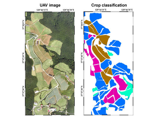
Figure 5.
Comparison of SVM-based classification results with ground-truth data: (a) ground-truth data; (b) August image with VNIR; (c) August image with VNIR and GK31 texture features; (d) six multi-temporal images with VNIR; and (e) six multi-temporal with VNIR and GK31 texture features.
Figure 5.
Comparison of SVM-based classification results with ground-truth data: (a) ground-truth data; (b) August image with VNIR; (c) August image with VNIR and GK31 texture features; (d) six multi-temporal images with VNIR; and (e) six multi-temporal with VNIR and GK31 texture features.

Figure 6.
Overall accuracy of classification results without texture features and with texture features generated from different kernel sizes for the cases using the August image and six multi-temporal images.
Figure 6.
Overall accuracy of classification results without texture features and with texture features generated from different kernel sizes for the cases using the August image and six multi-temporal images.

Figure 7.
Mean decrease accuracy (MDA) values of input spectral and texture variables with respect to kernel size: (a) August image; and (b) multi-temporal images. ME: mean; ENT: entropy; ASM: angular second moment; STD: standard deviation; HOM: homogeneity; DIS: dissimilarity.
Figure 7.
Mean decrease accuracy (MDA) values of input spectral and texture variables with respect to kernel size: (a) August image; and (b) multi-temporal images. ME: mean; ENT: entropy; ASM: angular second moment; STD: standard deviation; HOM: homogeneity; DIS: dissimilarity.

Figure 8.
Some texture features (GK31) in subareas of the August image.

Figure 9.
Temporal profiles of average normalized difference vegetation index (NDVI) values for three crops.
Figure 9.
Temporal profiles of average normalized difference vegetation index (NDVI) values for three crops.


Table 1.
List of unmanned aerial vehicle (UAV) image mosaics acquired in the study area in 2017.
| No. | Acquisition Date |
|---|---|
| 1 | 29 June |
| 2 | 12 July |
| 3 | 27 July |
| 4 | 25 August |
| 5 | 13 September |
| 6 | 21 September |
Table 2.
Crop classes and their respective area information in the study area.
| Classes | Total Area (ha) | Average Area per Parcel (ha) |
|---|---|---|
| Highland Kimchi Cabbage | 22.38 | 0.59 |
| Cabbage | 8.35 | 0.59 |
| Potato | 8.65 | 0.86 |
| Fallow | 3.08 | 0.31 |
Table 3.
Confusion matrices and accuracy statistics of some combination cases for the support vector machine (SVM) classifier. VNIR: visible and near infrared; UA: user’s accuracy; PA: producer’s accuracy; OA: overall accuracy; GK31: kernel size of 31 × 31.
Table 3.
Confusion matrices and accuracy statistics of some combination cases for the support vector machine (SVM) classifier. VNIR: visible and near infrared; UA: user’s accuracy; PA: producer’s accuracy; OA: overall accuracy; GK31: kernel size of 31 × 31.
| August Image: VNIR Spectral Information | ||||||
| Reference | Highland Kimchi Cabbage | Cabbage | Potato | Fallow | UA (%) | |
| Classification | ||||||
| Highland Kimchi cabbage | 3,074,131 | 342,355 | 49,838 | 84,726 | 86.57 | |
| Cabbage | 230,661 | 869,250 | 65,288 | 6627 | 74.18 | |
| Potato | 107,897 | 124,020 | 1,259,483 | 31,883 | 82.68 | |
| Fallow | 67,045 | 12,343 | 9497 | 375,166 | 80.85 | |
| PA (%) | 88.34 | 64.49 | 91.00 | 75.27 | ||
| OA (%) | 83.13 | |||||
| August Image: VNIR Spectral Information and GK31 Texture Features | ||||||
| Reference | Highland Kimchi Cabbage | Cabbage | Potato | Fallow | UA (%) | |
| Classification | ||||||
| Highland Kimchi cabbage | 3,317,807 | 237,669 | 22,404 | 44,455 | 91.59 | |
| Cabbage | 128,847 | 1,050,991 | 57,648 | 2636 | 84.75 | |
| Potato | 16,522 | 54,544 | 1,294,756 | 18,465 | 93.53 | |
| Fallow | 16,558 | 4764 | 9298 | 432,846 | 93.39 | |
| PA (%) | 95.35 | 77.97 | 93.54 | 86.85 | ||
| OA (%) | 90.85 | |||||
| Multi-Temporal Images: VNIR Spectral Information | ||||||
| Reference | Highland Kimchi Cabbage | Cabbage | Potato | Fallow | UA (%) | |
| Classification | ||||||
| Highland Kimchi cabbage | 3,421,871 | 46,150 | 11,031 | 41,618 | 97.19 | |
| Cabbage | 15,143 | 1,294,009 | 10,189 | 4185 | 97.77 | |
| Potato | 2092 | 4562 | 1,360,566 | 200 | 99.50 | |
| Fallow | 40,628 | 3247 | 2320 | 452,399 | 90.73 | |
| PA (%) | 98.34 | 96.00 | 98.30 | 90.77 | 97.30 | |
| OA (%) | 97.30 | |||||
| Multi-Temporal Images: VNIR Spectral Information and GK31 Texture Features | ||||||
| Reference | Highland Kimchi Cabbage | Cabbage | Potato | Fallow | UA (%) | |
| Classification | ||||||
| Highland Kimchi cabbage | 3,461,811 | 35,558 | 5349 | 16,199 | 98.38 | |
| Cabbage | 7159 | 1,309,847 | 5323 | 2337 | 98.88 | |
| Potato | 1346 | 792 | 1,372,686 | 186 | 99.83 | |
| Fallow | 9418 | 1771 | 748 | 479,680 | 97.57 | |
| PA (%) | 99.48 | 97.17 | 99.17 | 96.24 | 98.72 | |
| OA (%) | 98.72 | |||||
© 2019 by the authors. Licensee MDPI, Basel, Switzerland. This article is an open access article distributed under the terms and conditions of the Creative Commons Attribution (CC BY) license (http://creativecommons.org/licenses/by/4.0/).
Share and Cite
MDPI and ACS Style
Kwak, G.-H.; Park, N.-W. Impact of Texture Information on Crop Classification with Machine Learning and UAV Images. Appl. Sci. 2019, 9, 643. https://doi.org/10.3390/app9040643
AMA Style
Kwak G-H, Park N-W. Impact of Texture Information on Crop Classification with Machine Learning and UAV Images. Applied Sciences. 2019; 9(4):643. https://doi.org/10.3390/app9040643
Chicago/Turabian StyleKwak, Geun-Ho, and No-Wook Park. 2019. "Impact of Texture Information on Crop Classification with Machine Learning and UAV Images" Applied Sciences 9, no. 4: 643. https://doi.org/10.3390/app9040643
Note that from the first issue of 2016, this journal uses article numbers instead of page numbers. See further details here.