Single-Kernel FT-NIR Spectroscopy for Detecting Maturity of Cucumber Seeds Using a Multiclass Hierarchical Classification Strategy

Abstract

The maturity of seeds at harvest determines their intrinsic quality characteristics such as longevity and vigor, and these characteristics are dominant factors for seed quality evaluation in the seed industry. However, little information is available on how to identify and further classify the maturation stage of seeds in a way that is nondestructive, precise, rapid, and inexpensive, while also exactly meeting the need for the uniform control of seed performance in the seed industry to improve crop yield. This study demonstrated a nondestructive method for detecting seed maturity by using the single-kernel near-infrared spectroscopy (SK-NIRS) technique. The results showed that five classes of cucumber seeds with different maturation levels can be distinguished successfully. A tree-structured hierarchical classification strategy consisting of one soft independent modeling of class analogy (SIMCA) model and three partial least squares discriminant analysis (PLS-DA) models were proposed ending up with 99.69% of the overall classification accuracy and 0.9961 of Cohen’s kappa in the test set, and its predictive performance was superior to both SIMCA and PLS-DA for direct multiclass classification. SK-NIRS in combination with a multiclass hierarchical classification strategy was proved to be both intuitive and efficient in classifying cucumber seeds according to maturation levels.

1. Introduction

The intrinsic quality characteristics of seeds, such as longevity and vigor, depend on the maturation stage of seeds at harvest to a large extent, and they are dominant factors for successful crop production in the seed industry [1,2]. Particularly, obtaining seeds of high quality requires timely harvest at physiological maturity [3,4] before the seeds are fully ripe to ensure collection prior to dispersal [5] and to ensure maximum seed quality. During commercial seed production, maturity is usually estimated visually, relying on the experience of the growers [6]. Thus, two common scenarios often occur: harvesting too early may result in low yield and poor seed quality [7,8], while delaying harvest increases the risk of the seeds either shattering or deteriorating in the field. Even when the date of harvest is the same, there still exist the seed-to-seed differences that can occur on a plant or within an inflorescence, which will also result in physiological differences among seeds. Situations such as those described above contribute to the collection of a substantial proportion of seeds that are unsuitable for planting and long-term storage [9] due to their immaturity or low vigor.

However, in terms of conventional grading methods based on seed physical properties that are great enough to separate “good” from “inferior” seed such as size, shape, weight, color, and specific density [10], it is very difficult to recognize the relatively small differences exhibited by seeds at different maturation stages. Moreover, there are few studies on how to identify and further classify the maturation stage of seeds in a nondestructive, precise, rapid, and inexpensive way, and that is in line with the demand of the seed industry for uniformly controlling seed performance to improve crop yield [11]. A heuristic method based on measuring the chlorophyll fluorescence signals of intact seeds has been used to determine seed maturity and seed quality [12]. However, bulk sample measurement of this type cannot effectively identify single-seed differences, and no discrimination is possible.

Near-infrared spectroscopy (NIRS) analysis at the single-seed level followed by the use of a sorting mechanism could help increase sample uniformity [13] and has been successfully applied in grain, soybean, and corn [14,15,16]. It is widely known that near infrared spectral patterns, especially in the wavelength ranges of 1600–1800 nm and 2100–2200 nm, contain information about cis-unsaturation as well as about the carbon chain itself according to many reports [17,18,19]. Previous work has shown that the SK-NIRS approach coupled with chemometrics can be used to identify differences in viability in corn seeds [20]. Since the maturation stage of seeds at harvest can vary over a long time period, i.e., from 30 days after pollination (DAP) to 50 DAP, the differentiation of maturation stage results in different classes. Then, the challenge is whether the use of a combination of SK-NIRS and the chemometrics method can cope with this multiclass classification problem simultaneously. To date, this issue has been investigated with exploratory analysis; as far as we know, neither an available successful method nor satisfying classification results have been reported.

Before diving into the specific model building process, it is often necessary and helpful to do an exploratory data analysis, which may help to uncover relationships in the data, identify rules from the data, and discover latent data patterns [21]. Clustering is one such method to visualize and group observations based on similarities of the overall set of variables of interest, such as scores plot of the principal components in a principal component analysis (PCA) model, which can help develop a fine intuition of the latent group structure that will enlighten the forthcoming classification problem.

The most common approach to solving classification problems involving more than two classes, namely multiclass problems, involves decomposing the problem into several binary subproblems. Simultaneously predicting multiple classes can be accomplished by disposing of the binary classifiers in a tree-structured hierarchical way, referring to that general discrimination is performed first and becomes successively refined until the obtainment of the final classification. In general, the introduction of a hierarchy in a multiclass application may reduce the complexity involved in its solution [22]. For example, for the five-class classification problem in this study, the directed binary trees only need to train four predictors; this is the lowest number among the main decomposition strategies such as five predictors of one-versus-all and 10 predictors of one-versus-one. In addition, the nodes from the deepest levels involve less training data for the corresponding binary classifiers each time. Another important reason why it is preferred to use the decomposition strategy to deal with multiclass problems, even when they can also be directly handled by a single multiclass classifier, is that the former one is more robust and offers better behavior when significant differences are not always found [23].

The aims of this study were two-fold. One aim was to evaluate the potential of SK-NIRS analysis for identifying and interpreting the distinctions in cucumber (Cucumis sativus L.) seeds harvested at five different periods combined with the analytical results of relative chemical concentration; the other was to propose a hierarchical classification strategy to predict these five maturation stages simultaneously. In the proposed hierarchical model, a set of sequential subclassifiers was generated using the chemometrics methods of the SIMCA and PLS-DA. Together with the exploratory data analysis such as PCA, this hierarchical multiclass classification scheme was able to provide both an intuitive classification process and precise predictive results. In order to better evaluate the effectiveness of this hierarchical classification strategy, a direct SIMCA and PLS-DA model for multiclass classification had been also developed on their own to compare the predictive performances based on a set of classification metrics.

2. Materials and Methods

2.1. Seed Preparation

Seeds of an orthodox Chinese cucumber (Cucumis sativus L. cv. Yuefeng) were produced outdoors in Baiyun District of Guangzhou, Guangdong Academy of Agricultural Sciences, China, in the spring–summer season of 2018. During pollination, some flowers were tagged, and fruits were randomly sampled from the two rows of the plot; of these, the 20 fruits used in the current study were harvested at 25, 30, 35, 40, and 45 days after pollination (DAP). The normal time for seed harvest in the region is approximately 40 DAP and depends on the specific conditions of the cultivar, field management, and weather.

The 20 fruits were divided into five groups on five-days intervals; each group contained four fruits that were harvested at the same time. Each fruit was coded, and it was then split open. The seeds, together with the mucilage tissues, were extracted from the placental tissue by hand and placed in a nylon bag. The seed mixture in the bag was washed vigorously in tap water with moderate kneading until the seeds could be easily separated. Then, the seeds were immersed in water, and the sample was filtered approximately three times; only the seeds that sank to the bottom of the container of water were retained. After cleaning, the seeds were dried outdoors for three days under ambient air conditions.

Considering the conformity of seeds in each class and the seed-filling phase during the maturation of seeds, the representatives of seed samples in five classes have been determined by the average kernel weight such as the kernel weight in 100 seeds. According to this principle, one representative seed lot sample was selected from each four-member group to provide a typical seed lot sample for each of the five groups. Thus, five seed samples denoted MS1, MS2, MS3, MS4, and MS5, representing five maturation stages (MS) at harvest, were obtained. Seed moisture content was determined using a moisture meter (CTR-500ET, Suncue Company Ltd., Japan); all seeds reached an equilibrium moisture content (%) of 12.56 ± 0.32 before the collection of the NIR spectra.

2.2. Spectral Data Acquisition

A diffuse reflectance measurement method was used to collect the NIR spectra of individual cucumber seed kernels. Unlike other endosperm-containing seeds (e.g., corn) that have been shown to display obvious spectral variance between the germ and endosperm side, no distinct dual sides exist in cucumber seeds. Given that various spectral variances independent of chemical composition are produced by differences in seed curvature [24], shape [13], roundness, and thickness [25], an integrating sphere was utilized to improve the signal-to-noise ratio, thereby alleviating the heterogeneity effect.

All 656 seeds were scanned individually using a Fourier transform near-infrared spectrometer (Antaris II FT-NIR Analyzer, Thermo Scientific Co., Waltham, MA, USA). Each sample label was named in sequential order during the spectra collection. The spectrum of each kernel was recorded in the wavenumber range from 10,000 to 4000 cm⁻¹ (1000–2500 nm) at 8 cm⁻¹ intervals; a total of 778 points were recorded for each spectrum. The NIR reflectance spectra were calculated as log (1/R), where R represents the reflectance. A schematic diagram of the SK-NIRS can be found in previous work [20]. Averaged spectra from 16 successive scans of each individual seed were obtained for further analysis.

2.3. Chemical Composition Measurements

Considering the protein (33.8%), fat (45.2%), carbohydrate (10.3%), and crude fiber (2.0%) composition of cucumber seeds [26], the former two dominant constituents were analyzed in this study. Chemical analysis of each seed category sample was conducted according to the standard methods of the International Standard Organization (ISO). According to the correlated international standard [27], the Dumas combustion principle was used to determine the nitrogen content of the samples using an elemental analyzer (rapid N exceed, Elementar, Germany). Crude protein was calculated using a conversion factor of 6.25. The results are expressed as percent concentration. It should be noted that at least three replicates of chemical measurements are often required to define the error bars of corresponding compound concentrations. However, due to the sample selection principle used in the experimental design of this study, the number of sample seeds in five classes are relatively limited and in short supply; thus, they are not able to cover all the usage in three replicates during the chemical composition measurements.

The fatty acids present in seed oil were subjected to methyl esterification; then, the determination of fatty acid methyl ester (FAME) composition and the quantification of individual FAMEs were performed on a gas chromatography-mass spectrometry (GC-MS) system (7890B-5977A, Agilent J & W Scientific, Santa Clara, CA, USA). The chromatographic separation of FAME was achieved with the use of an HP-5MS elastic quartz capillary column (30 m × 0.25 mm). The working conditions were as follows: the carrier gas was highly purified helium (99.9995%, Air Liquide Industrial Gas Co., Ltd., Guangdong Province, China); the flow rate was 1.0 mL/min; the split ratio was 50:1; the temperature program of the GC was 50 °C (held for 1 min), increased to 200 °C at a rate of 10 °C/min (held for 5 min), increased to 220 °C at a rate of 5 °C/min (held for 10 min), and finally increased to 280 °C at a rate of 10 °C/min. The MS program scanned a mass range of 30–450 amu at an ionization voltage of 70 eV. The ion source temperature was set at 230 °C. Individual FAMEs were identified by comparing their retention times with those of FAME standards and quantified using the calibration curves established for individual FAMEs.

2.4. Dataset Partition and Parameter Settings

MATLAB (MathWorks, Natick, MA, USA) with PLS Toolbox v.8.2.1 (Eigenvector Research, Inc., Manson, WA, USA) was used to conduct the NIR spectral data analysis. The independent test set samples were selected using the Kennard and Stone duplex method [28]; for each class, 50% of the samples were assigned to the training set and 50% were assigned to the test set (a split ratio of nearly 1:1). The sample composition of four classification models for each class (positive or negative) is shown in

Table 1. The number of samples used in four classification models in both training and test phases. PLS-DA: partial least squares discriminant analysis, SIMCA: soft independent modeling of class analogy.

	SIMCA		PLS-DA 1		PLS-DA 2		PLS-DA 3
	P	N	P	N	P	N	P	N
	MS1	MS2,3,4,5	MS2	MS3,4,5	MS3	MS4,5	MS4	MS5
training	90	239	52	187	61	126	49	77
test	90	237	52	186	60	125	49	76

P: positive class; N: negative class.

. The preprocessing method applied to the NIR spectral datasets was the first Savitzky–Golay [29] derivative (second polynomial with a filter width of 15) followed by mean centering to remove offsets from the spectral data.

Cross-validation is a very useful tool that enables an assessment of the optimal complexity of a model such as the number of principal components in a PCA model. In this study, samples of each class randomly compose its correlated dataset; thus, it is appropriate to adopt the Venetian blinds method to perform cross-validation. Moreover, because this method requires that the variables are correlated, it is particularly suited to NIR data [30]. This approach includes a set of subvalidation procedures, each of which involves the removal of 10% of the samples from a total dataset; then, a model is built with the remaining 90% samples in the dataset and is applied to the removed samples. The optimal number of latent variables (LVs) in the classification model was determined using the root mean square error of cross-validation (RMSECV).

2.5. SIMCA and Statistics of PCA Models

PCA is often the first step of the exploratory analysis to detect groups in high-dimensional datasets. The SIMCA method based on disjoint PCA modeling consists of a collection of PCA models, one for each class in the calibration set [31]. In the test phase, the unseen instance will be recognized as a member of a class if it is similar enough to the other members; else, it will be rejected. Specifically, measures of Q residuals and Hotelling’s T² of a sample are compared to a PCA submodel in SIMCA. It is often useful to determine whether a sample is a member of a particular group based on the lack-of-fit statistic of Q, which accounts for the residual part of the variation that is not explained by the PCA model.

For a training matrix X consisting of m rows (samples) and n columns (variables), the following equation describes the relationship between the data and the PCA model:

$${\mathit{X}=\mathit{TP}}^{\mathrm{T}}+\mathit{E}$$

(1)

where T is the scores matrix of all the training samples, P is the loadings matrix, and E is the residual matrix.

Q residuals are calculated as the sum of squares of each row (sample) of E, i.e., for the $i\mathrm{th}$ sample in X (${\mathrm{x}}_i$),

$${\mathit{Q}}_i=e_i{e}_i^T=x_i \left(\mathit{I}-{\mathit{P}}_k{\mathit{P}}_k^T\right) x_i^T$$

(2)

where $e_i$ is the $i\mathrm{th}$ row of E, ${\mathit{P}}_k$ is the matrix of the k loadings vectors retained in the model (where each vector is a column of ${\mathit{P}}_k$), and I is an identity matrix of the appropriate size (n by n).

Hotelling’s T² is the sum of the normalized squared scores and is defined as

$${\mathit{T}}_i^2=t_i{\lambda }^{-1}{t}_i^T=x_i{\mathit{P}}_k{\lambda }^{-1}{\mathit{P}}_k^T{x}_i^T$$

(3)

where $t_i$ refers to the $i^{\mathrm{th}}$ row of ${\mathit{T}}_k$ in the m by k matrix of scores from the model, and λ is a diagonal matrix containing the eigenvalues (${\lambda }_1$ through ${\lambda }_k$) corresponding to the k principal components retained in the model.

Q is a measure of the distance from a sample point to its projection onto the k factors retained in the model; a large Q value indicates that unusual variation exists outside the model. T² represents a measure of the variation in each sample within the model; a large T² value indicates that unusual variation exists within the model.

2.6. PLS-DA Method and Classification Metrics

The interference and overlapping of the spectra information may be solved by using PLS regression, which finds a linear regression model by projecting the predicted variables and the observable variables to a new space. It will try to find the multidimensional direction in the X space that explains the maximum variance direction in the Y space. If the dependent variable does not assume continuous values as in quantitative analysis but discrete ones (for example, 0 for the negative class or 1 for positive class), then it gives rise to the PLS-DA method.

In the case of single-response y and p predictors, a PLS regression model with n latent variables (LVs) can be expressed as follows:

$${\mathit{X}=\mathit{TP}}^{\mathrm{T}}+\mathit{E}$$

(4)

$$\mathit{y}=\mathit{Tb}+\mathit{f}$$

(5)

where b explains the relationship between y and T, f stands for random errors of y, and a weight matrix W (p × n) is obtained to make the Euclidean norm of f as small as possible. The variable importance in projection (VIP) scores estimate the importance of each variable in a PLS model, and for the jth variable, it can be calculated as:

$${\mathit{VIP}}_j=\sqrt{\frac{p{{\displaystyle \sum }}_{k=1}^n{\mathit{b}}_k^2{\mathit{t}}_k^{\mathit{T}}{\mathit{t}}_k{{(\mathit{w}}_{jk}{/\left|\right|\mathit{w}}_k\left|\right|)}^2}{{{\displaystyle \sum }}_{k=1}^n{\mathit{b}}_k^2{\mathit{t}}_k^T{\mathit{t}}_k}}$$

(6)

and because the average of the squared VIP scores equals one, the thumb rule of “greater than one” is generally used as a criterion for variable selection [32].

The confusion matrix is often used to evaluate the performance of binary classification models. For example, if the MS4 class (with a y value of 1) was identified as positive, the corresponding MS5 class (with y values of 0) were identified as negative. The true positive (TP) is the number of MS4 samples correctly classified as MS4, and the true negative (TN) is the number of MS5 samples correctly assigned as MS5. The false negative (FN) is the number of MS4 samples incorrectly classified as MS5, and the false positive (FP) is the number of MS5 samples incorrectly assigned as MS4. TP and TN lie within the main diagonal of the confusion matrix. The classification accuracy rate (Acc) is calculated as:

$$\mathrm{Acc}=\frac{\mathrm{TP}+\mathrm{TN}}{\mathrm{TP}+\mathrm{TN}+\mathrm{FP}+\mathrm{FN}}.$$

(7)

Cohen’s kappa is an alternative measure that can be used to determine the accuracy rate for multiclass problems. This measure compensates for random hits and possesses the advantages of being both useful and simple for measuring classifier’s observations with respect to the degree of agreement of multiclass classification problems. It is more convenient to calculate Cohen’s kappa in terms that are based on counts rather than probabilities [33]. For an m-class problem,

$$\mathrm{Kappa}=\frac{N{{\displaystyle \sum }}_{i=1}^m{C}_{ii}-{{\displaystyle \sum }}_{i=1}^m{C}_{.i} C_{i.}}{N^2-{{\displaystyle \sum }}_{i=1}^m{C}_{.i} C_{i.}}$$

(8)

where N is the number of test samples, $C_{ii}$ is the number of TPs for each class in the main diagonal, $C_{.i}$ is the sum of counts in the $i\mathrm{th}$column, and $C_{i.}$ is the sum of counts in the $i\mathrm{th}$ row.

The calculated value of Cohen’s kappa ranges from −1 (total disagreement) through 0 (random classification) to 1 (complete agreement). The closer the kappa value is to 1, the better the performance of the hierarchical classification scheme.

3. Results and Discussion

3.1. SK-NIRS Spectra and Correlated Chemical Concentrations

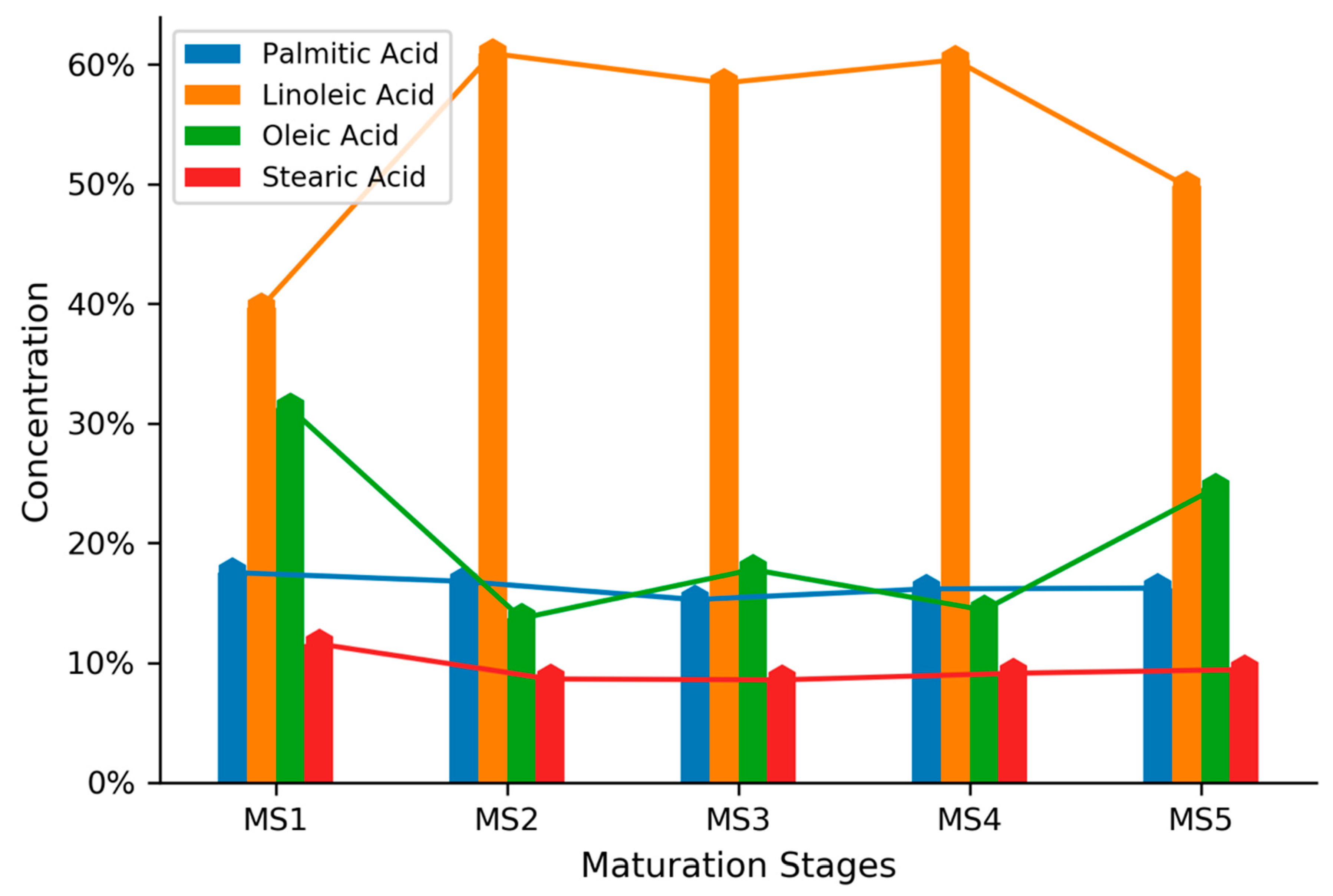
Figure 1 described the qualitative analysis results of four main fatty acids compositions in seed oils as the maturation stages increased. It also showed the crude protein percent concentration of seed at five different maturation stages. The measured concentrations of crude protein had a slight increase between the MS2 (32.36%) and MS3 (34.57%) phase, and after that stayed relatively steady around 33.9%. It showed that two saturated fatty acids (palmitic acid and stearic acid) concentrations remained nearly constant as the maturation stage of the cucumber seeds progressed. However, the concentrations of two unsaturated fatty acids showed obvious fluctuations as the maturational stage increased. Specifically, the maximum concentration of oleic acid occurred in MS1; it then decreased steeply in MS2, remained steady in MS3 and MS4, and finally increased greatly in MS5. In contrast, the concentration of linoleic acid, which is the dominant constituent of oil in cucumber seeds, was completely opposite to that of oleic acid. This strong negative relationship between oleic acid and linoleic acid in cucumber seeds agreed with that in the study of Ngure et al. [34]. In terms of the average spectra in Figure 2b, the most distinctive maturational stages were found in MS1 and MS5. Considering that cucumber seeds are very rich in oil (nearly 40%), the obvious differences in the concentrations of oleic and linoleic acids may account for the differences in absorption of incident light in the near-infrared region, especially in MS1 and MS5.

As shown in Figure 2, the main absorption peaks of cucumber seeds were observed at approximately 1210 nm, 1471 nm, 1726 nm, and 1929 nm in the average SK-NIRS spectra of five maturational stages. According to the interpretations of Jerry and Lois [35], the overlapping peak with a maximum of approximately 1210 nm results from the second overtone arising from the C–H stretching mode; the absorption band at 1471 nm is characteristic of the first overtone N–H stretching; the absorption peak around 1726 nm is due to the first overtone of C–H stretching; the absorption band centered near 1929 nm results from a combination of O–H stretching and H–O–H bending. These absorption properties of cucumber seeds may be explained by the high protein and oil content of the seeds [17] and the differences in the specific composition of the seeds as the maturation stage of the seeds increases. In addition, there was an apparent negative correlation between the height of the absorption peaks and the maturation stage of the seeds. It would make sense based on the fact that the cucumber seeds get thicker and thicker as their maturation stage increases. Thus, there is more incident NIR light reflected back to the detector, and the NIR absorption intensity decreases as the maturation stages increase. As far as we know, little information is available about how the maturation stage affects the absorption of incident light in the near-infrared region. The NIR spectra contain information from all the chemical constituents of the sample, and direct interpretation of the absorbance values obtained from complex mixtures such as those present in intact kernels is difficult.

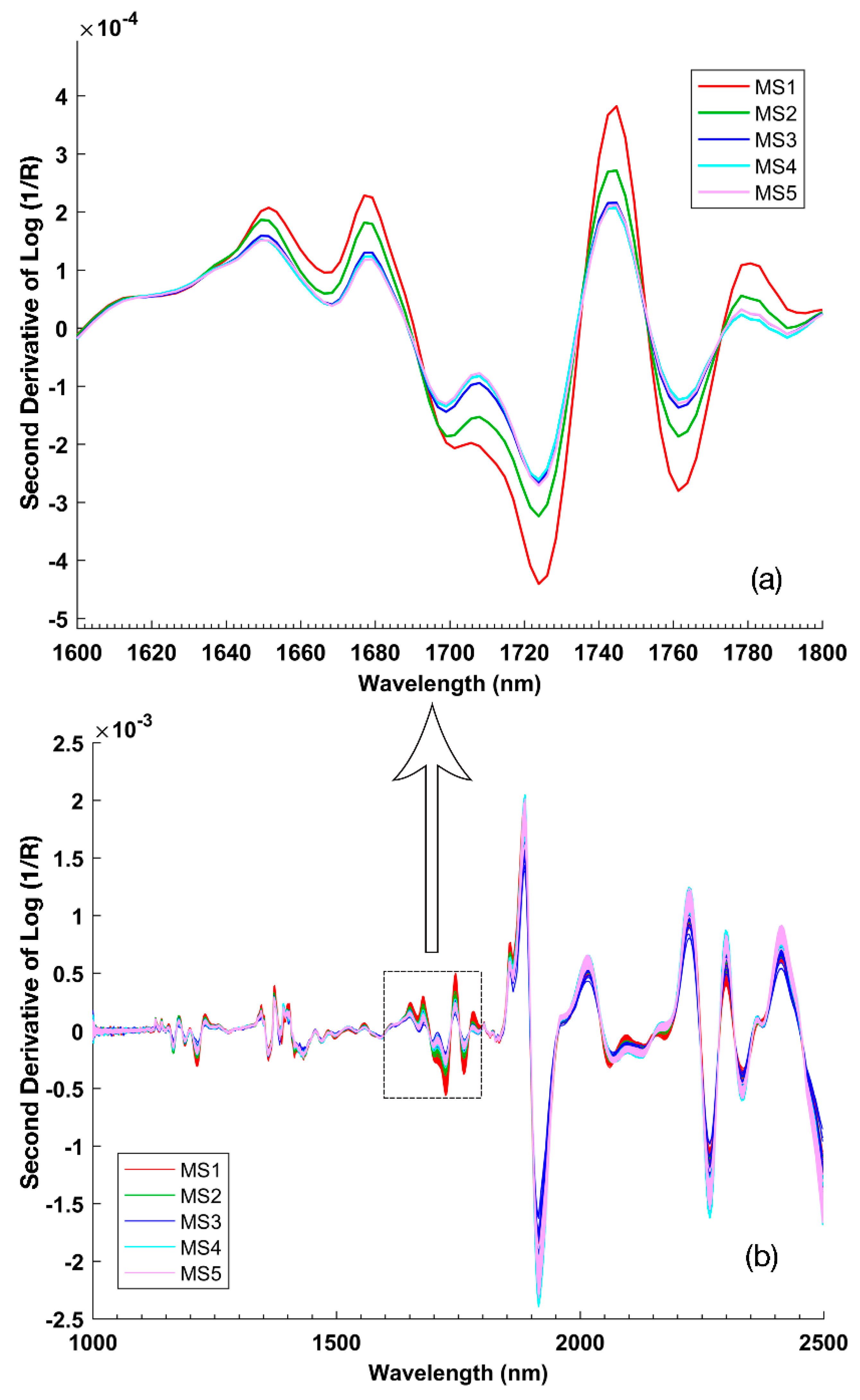
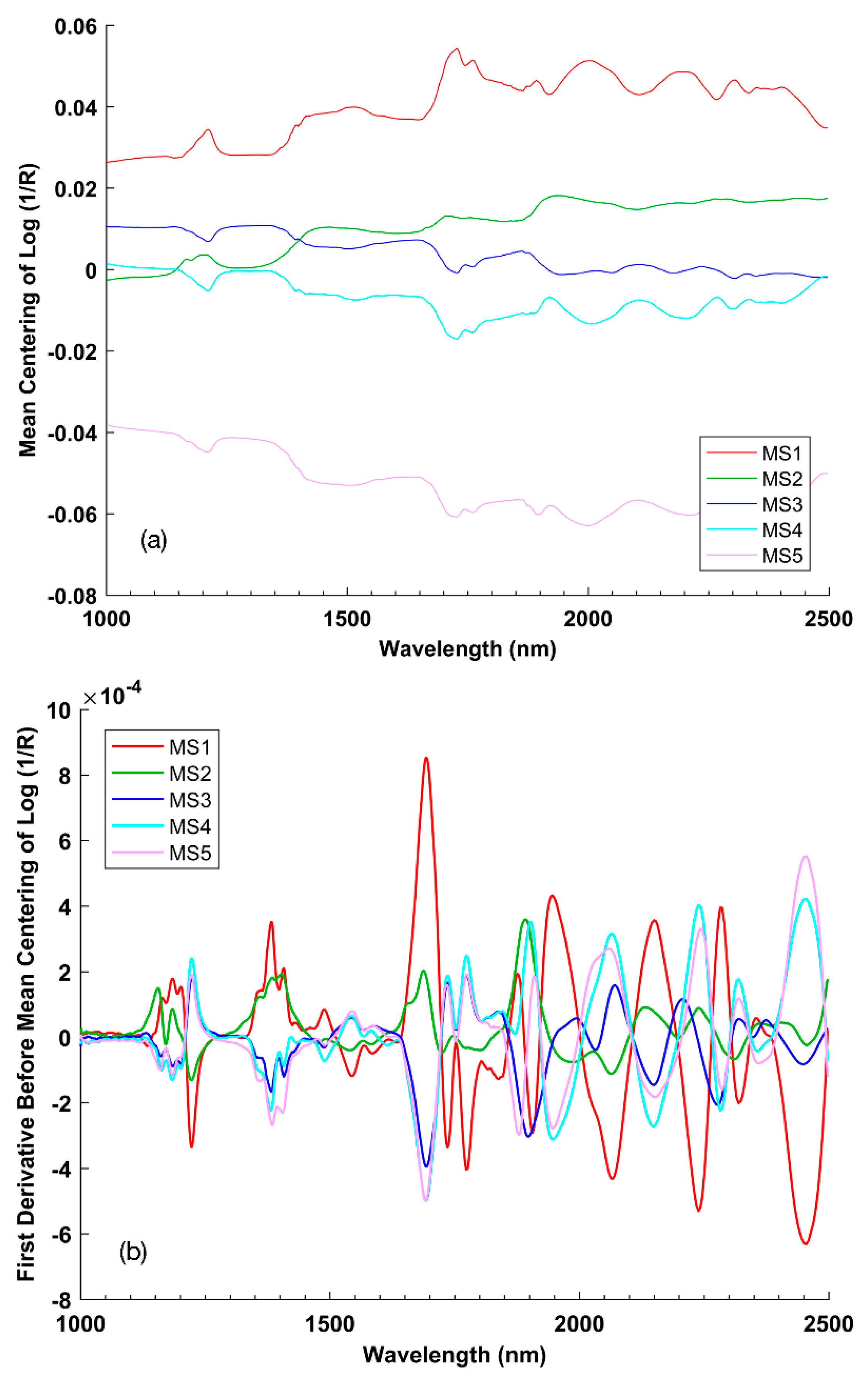
The raw spectral features can be enhanced using the second Savitzky–Golay derivative (second polynomial with a filter width of 15), which has a trough corresponding to each peak in the raw spectra. The second-derivative SK-NIRS spectra of all regions and one special interval are plotted in Figure 3.

As the peak value at a wavelength in the raw spectra goes up much higher, the trough value at the corresponding wavelength in the second derivative spectra moves downward much deeper. Particularly, the position of the minima correlates with the position of the peaks in the raw spectra. The 1600–1800 nm wavelength region, which possesses the most distinctive absorption features, shows two major troughs in the vicinity of 1724 and 1761 nm [17,18,19]. These troughs are characteristic of the first overtone of the C–H stretching vibration of methyl, methylene, and ethylene functional groups. This region of the NIR spectrum has been studied by numerous authors, and this pattern is considered to be one of the main features of oils. For example, oils rich in monounsaturated fatty acid have a peak centered near 1725 nm that is attributed to oleic acid [36]. Oleic acid is highly concentrated in cucumber seeds. This absorption peak was also observed in our study. Therefore, the obvious variation in the levels of the dominant fatty acids in cucumber seeds, linoleic acid, and oleic acid may account for the substantial absorption features observed in this region.

3.2. The Exploratory Analysis

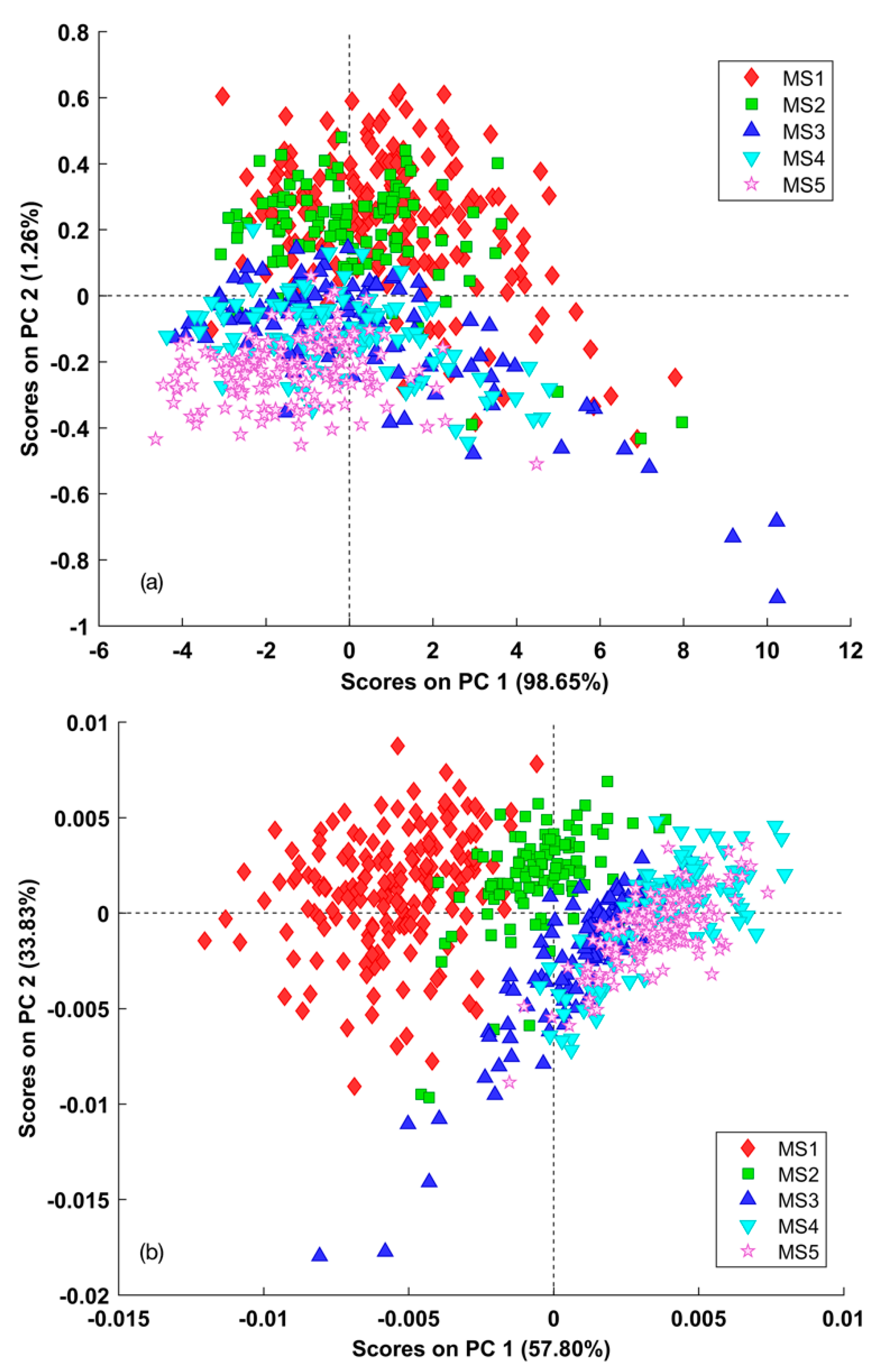
To determine whether the raw datasets contain sufficient information to allow us to distinguish the groups, an exploratory analysis was performed in this study. All 656 instances in the dataset were subjected to exploratory data analysis in a PCA model at a confidence level of 95%. PCA is generally applied to data that has been “mean-centered” by subtracting off the original mean value of each column. In addition to this basic preprocessing method, derivatives as a common method to remove unimportant baseline signals from samples combined with the mean centering are also used as a contrast. Figure 4 shows the two different preprocessed data viewed by classes; one is using the preprocessing method of mean centering (a), the other instead firstly uses the Savitzky–Golay first derivative (second polynomial with a filter width of 15), and then goes through the mean centering method and finally shows in (b). It could be seen from Figure 4 that both methods were able to distinguish samples of five classes at most bands, but the latter one uniquely had one advantage: by taking the first derivative, it had removed the predominant background variation from the original data such as bands between 1000 and 1150 nm.

Figure 5 presents scores plots showing the instances viewed by classes projected on the top two principal components of the relative PCA model.

Not any clear independent cluster could be found on the scores subplot (a); different classes just highly overlapped together. This can also be inferred from Figure 4a, the preprocessed data by the method of the mean centering does not have sufficient information that could be used to exhibit the differences between classes. In contrast, lots of absorption features existed in samples of five classes can be found in Figure 4b: the 1600–1800 nm region, 1900 nm, etc. In addition, three obvious groups can be identified from the scores subplot (b). That is, samples in the MS3, MS4, and MS5 classes overlapped and formed a cluster, while samples in the MS2 class and those in the MS1 class formed independent clusters. To figure out which correlative variables are responsible for the scores subplot (b), Figure 6 shows the loadings plot on the top two principal components of the relative PCA model.

From the relative scores subplot in Figure 5b, it could be found that samples of MS3, MS4, and MS5 have positive correlations with the first principal component (PC 1). Moreover, the wavelengths where samples of MS3, MS4, and MS5 classes are distinguished from those of MS1 and MS2 in Figure 4b are almost the same as those where PC1 is different from PC2 in Figure 6. It indicates that this preprocessing method helps reveal the hidden distinctions of different maturation classes. So, it is reasonable to use this preprocessing method in the following classification models.

Another great reward that this explorative analysis can bring is to provide an intuition that helps build the tree-structured hierarchical classification scheme. Taking an overview of the group structure, the relationship shown in the scores subplot in Figure 5b, a PCA submodel of SIMCA could be constructed to separate the MS1 class from the rest of the samples using sample projections on the Q statistic of this submodel. For the remained four unassigned classes, it may be appropriate to successively assign one class upon one binary classifier, and it seems that PLS-DA is a good candidate.

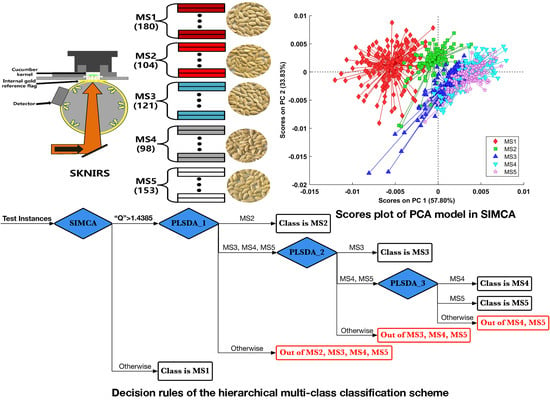
3.3. Root Rule Node: Distinguish MS1 Class from the Rest by the First PCA Submodel in SIMCA

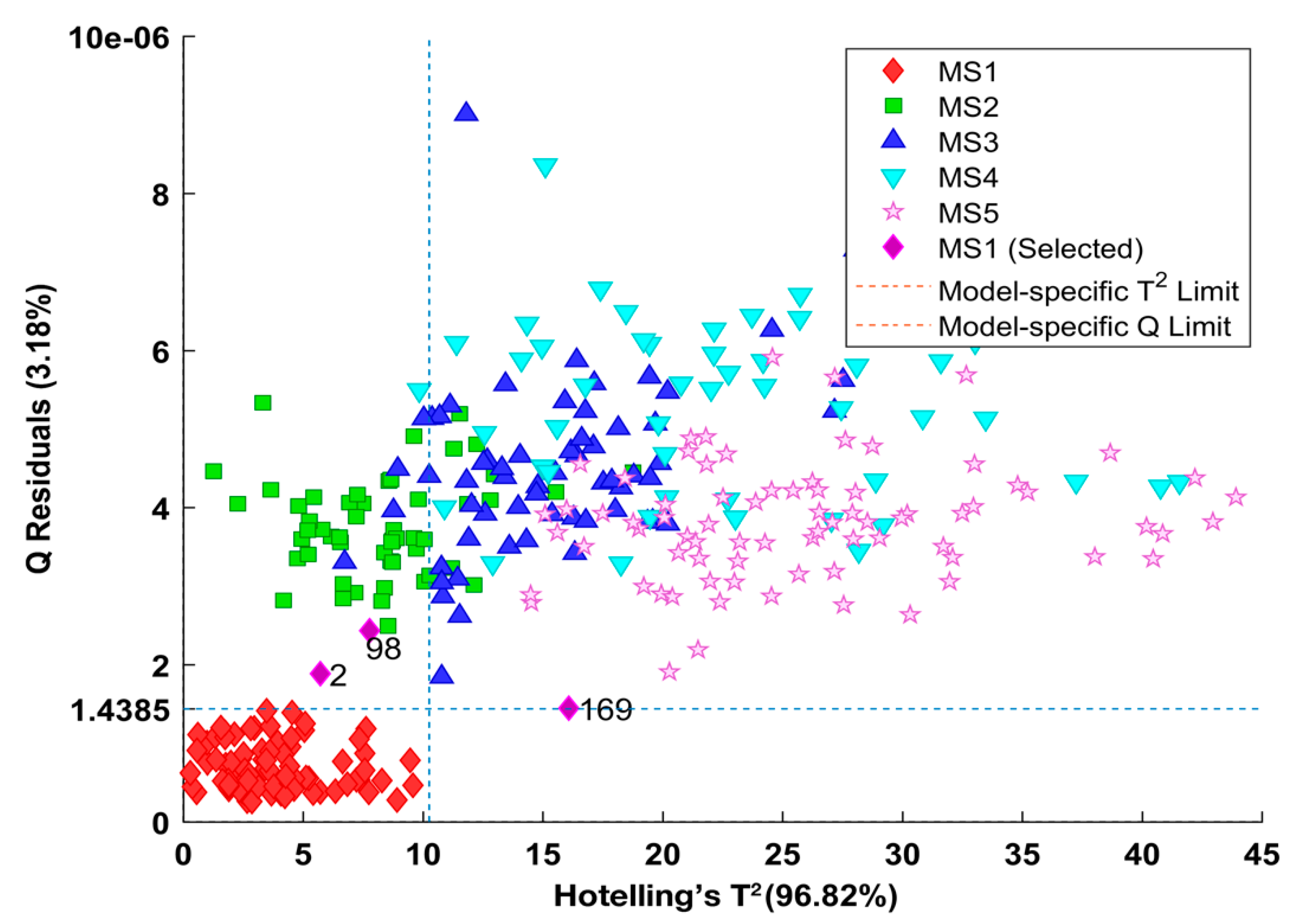
A SIMCA model consists of a collection of PCA submodels, which is typically one for each class in the dataset, but it is also possible to build a PCA submodel on combined classes. In this context, the first PCA submodel with four PCs had been fitted on samples only belonging to the MS1 class; then, it was added to SIMCA. After that, another PCA submodel with four PCs fitted on the rest of the samples that combined all the remaining classes had also been built and added to SIMCA. Finally, these two PCA submodels were assembled in the SIMCA model.

Both submodels were trained using the same preprocessing method consisting of the first Savitzky–Golay derivative (second polynomial with a filter width of 15) followed by mean centering. The configurations in cross-validation of the Venetian blinds method included 10 splits and one sample per split. Based on the value of RMSECV, the optimal number of principal components (PCs) in these two models was selected, and both were equal to four. The performances of these two submodels in the training and test phases are shown in

Table 2. Confusion matrix of the SIMCA model during its training and test phases.

Predicted Class	Actual Class
	Train		Test
	MS1	MS2, MS3, MS4, MS5	MS1	MS2, MS3, MS4, MS5
MS1	87	10	90	0
MS2, MS3, MS4, MS5	3	229	0	237

.

From Table 2, it can be found that during the training phase, the first PCA submodel in SIMCA had misclassified three samples of MS1 as the remaining class; despite this case, this PCA submodel perfectly identified all the members of MS1 in the test phase. It also can be verified in plots featuring the classification results of this PCA submodel both in the training and test phases, as shown in Figure 7.

In Figure 7a, those members of the MS1 class that had been misclassified as the remaining class were selected and labeled with their filename labels. However, all the members belonging to the MS1 class in the test phase were precisely classified as MS1 in Figure 7b. Furthermore, to incorporate this PCA submodel as the root decision node into the hierarchical model structure, the projection test-based rule that tells how to choose a branch based on the predictions of the given model from the input data needs to be defined.

This PCA submodel had a specific Q limit that equaled 1.4385e-06, as shown in Figure 8, and according to this Q limit, this model had misclassified three samples of the MS1 class; their labels were just the same with those observed in Figure 7a. That is to say, this defined test condition “Q >1.4385 ×10⁻⁶” would work well to specify which given branch would be selected after the root decision node.

3.4. Rule Nodes: Subdivide the Four Remaining Classes by Three Increasingly Specific PLS-DA Classifiers

All three PLS-DA classifiers used here were binary; for example, the first PLS-DA classifier denoted PLS-DA 1 could only separate members of the MS2 class from those of a general category consisting of MS3, MS4, and MS5. Likewise, the second PLS-DA classifier denoted PLS-DA 2 separated the MS3 class from the remaining MS4 and MS5 class. Finally, the last PLS-DA classifier denoted PLS-DA 3 separated the MS4 class from the MS5 class.

The same preprocessing method (the first Savitzky–Golay derivative (second polynomial with a filter width of 15) followed by mean centering) was used to build these three PLS-DA classifiers. The configurations used in the cross-validation of the Venetian blinds method were 10 splits, featuring one sample per split. The correlated optimal LVs were selected based on the value of the RMSECV. The confusion matrices of the training and test samples in the three PLS-DA models are shown in

Table 3. Confusion matrix of the training samples in the three PLS-DA models.

PLS-DA 1			PLS-DA 2			PLS-DA 3
Predicted Class	Actual Class		Predicted Class	Actual Class		Predicted Class	Actual Class
	MS2	MS3,4,5		MS3	MS4,5		MS4	MS5
MS2	52	0	MS3	59	1	MS4	49	0
MS3,4,5	0	187	MS4,5	2	125	MS5	0	77

and

Table 4. Confusion matrix of the test samples in the three PLS-DA models.

PLS-DA 1			PLS-DA 2			PLS-DA 3
Predicted Class	Actual Class		Predicted Class	Actual Class		Predicted Class	Actual Class
	MS2	MS3,4,5		MS3	MS4,5		MS4	MS5
MS2	52	0	MS3	59	3	MS4	49	0
MS3,4,5	0	185	MS4,5	1	122	MS5	0	76

, respectively.

In terms of the results shown in Table 3 and Table 4, the performances of the first and last PLS-DA classifiers in both the training and test phases were perfect; all the samples were correctly classified in both the training and test phases with the anti-diagonal elements all equal to zero. Nevertheless, the performance of the second PLS-DA classifier was inferior to that of the others. As shown in Table 3, in the training phase, it had an FN value of 2, indicating that 2 of the 61 samples in the MS3 class were incorrectly classified as belonging to the general category consisting of the MS4 and MS5 classes. The FP value of 1 showed that 1 of the 126 samples in the general category consisting of MS4 and MS5 classes were incorrectly assigned to the MS3 class. Furthermore, this problem was a little bit more serious in the test phase with a large FP value of 3 in Table 4; actually, the 48th and 85th samples from the MS4 class and the 119th sample from the MS5 class were incorrectly identified as belonging to the MS3 class. In addition, noticing that FN value was 1, it indicated that the 117th sample from the MS3 class had been misclassified as belonging to the MS4 class.

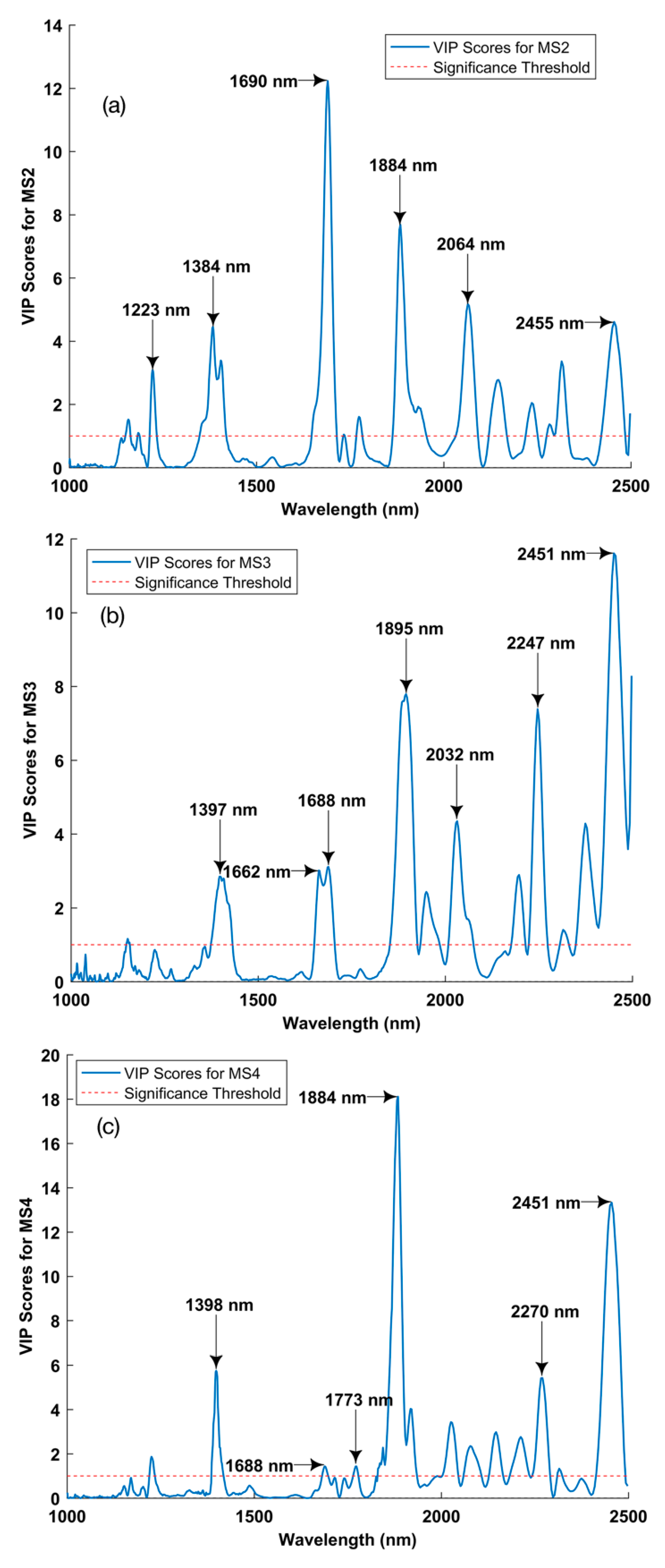
In the training phase, three PLS-DA models have achieved classification accuracy rates of 100%, 98.4%, and 100%, respectively. As for the testing phase, the corresponding classification accuracy rates are 100%, 97.8%, and 100%. All these three PLS-DA models have achieved very nice predictive results on correlated sample classes in general, but it is still unclear which variables are responsible for these good performances. VIP scores can estimate the importance of each variable in the projection used in a PLS-DA model. Specifically, a variable with a VIP score close to or greater than one (significance threshold) can be considered important in the given model. The VIP scores of three PLS-DA models regarding specific classes are shown in Figure 9.

In terms of the bands annotated in Figure 9, only a few of them have been publicly reported as meaningful in bands assignment [35]. Firstly, absorption bands associated with protein as amides include a peak at 1688 nm explained by one functional group of CONH₂ specifically due to peptide sheet structures; Secondly, it is reported that poly(ether urethane urea) has a band assignment at 1690 nm, which is due to the C–H aromatic first overtone. Finally, a second overtone of the asymmetric bending mode in the methyl functional group is expected to be at 2270 nm. It could be found that the 1600–1800 nm NIR region both contributed a lot to the VIP scores of all three PLS-DA models and did have a solid basis in band assignment. The absorption bands of cis-unsaturation and the carbon chain length of the fatty acid moieties in oil appear in the NIR wavelength region, especially around 1600–1800 nm [17,18,19], and combined with the observations from Figure 1 and Figure 3, which show that the samples at five classes do have fluctuations and distinctions, so it can be inferred that this special region may help provide good features so that the PLS-DA models can better classify these samples.

3.5. The Hierarchical Classification Structure

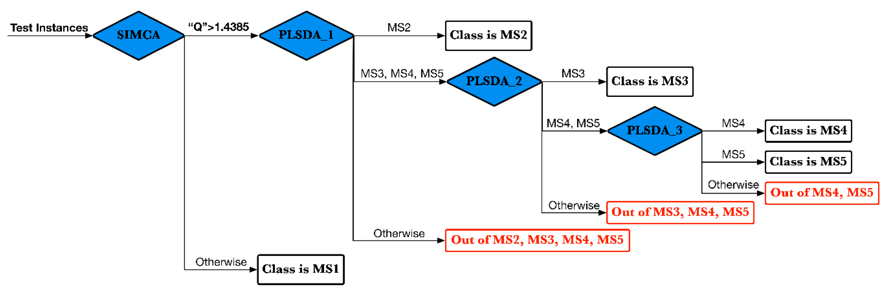
A classification problem including five classes can be solved combining one projection test-based rule node and three classification test-based rule nodes in a tree-structured hierarchical way, as shown in Figure 10. For each of the three classification rule nodes, the number of branches of a node is defined by the number of classes defined in the classification model. There will be one branch for each class defined, plus the additional “otherwise” branch used if none of the other classes is selected.

In the test phase, all of the unseen instances (test instances) flowed from left to right and are first passed through the root decision node; the results from this node are used to select one of the branches to the immediate right of the root node. Four rule nodes (blue diamonds) are arranged from left to right; these are the projection rule of the first PCA submodel in SIMCA and three classification rules based on the first, second, and last PLS-DA model, respectively. Specifically, the test condition of the first projection rule is shown here; that is, instances that had a Q residual value larger than the Q limit (shown in Figure 8) would be subject to the right classification rule node. If this test condition was not met, each instance would be output with a string indicating its true class (black rectangle). For each of the three PLS-DA classification rule nodes, there are always three branches representing the output categories: the upper branch represents the positive class, the middle branch includes the negative class, and the lower branch returns the “otherwise” string (red rectangle). Clearly, the test instances of the four classes are classified in a top–down approach. At first, all four classes are subject to the second rule (based on the outputs of the first PLS-DA classifier); then, three remaining classes enter the next classifier (based on the outputs of the second PLS-DA classifier), and finally only two classes are subject to the last classifier (based on the outputs of the last PLS-DA classifier).

Once the overall hierarchical decision rule has been set up, it can be easily applied to the test set including samples of all five classes, and the prediction results will be a list containing outputs for each row of the test data. In fact, these one-for-all prediction results are just the same as those produced by the four separated models defined above.

Overall, the prediction results were very satisfying; all the samples in the MS1 and MS2 classes were correctly predicted as the corresponding classes. The 117th sample in the MS3 class was incorrectly predicted as belonging to the MS4 class. Additionally, the 48th and 85th samples in the MS4 class were incorrectly predicted as belonging to the MS3 class. The 119th sample in the MS5 class was incorrectly predicted as belonging to the MS3 class. It seems that the PLS-DA model is prone to get confused with those samples whether they are belonging to the MS3 class or the MS4 class. This predictive performance is very similar to the performance that occurs in the training process; for example, the samples in the MS3 and MS4 classes overlap heavily in the PCA scores plot shown in Figure 5b. Furthermore, the misclassification rate of the MS3 and MS4 classes is obviously higher than that of the other classes, as can be seen from the confusion matrices for both training and test in Table 3 and Table 4. Taken together, these findings tend to show that the MS3 and MS4 samples are very similar in terms of their absorption properties in the near-infrared region. Reviewing the dominant chemical constituents of the samples in these two classes as shown in Figure 1, it is clear that the two classes are very similar in their content of both oil and protein, which together account for more than 75% of the seed composition. Therefore, the hierarchical classification scheme brings more intuitions to interpret some inner relationships of complicated classification problems by breaking it down into subgroups with individual models handling the increased detail of the problem.

For a five-class classification problem, it is appropriate to evaluate the classification performance using Cohen’s kappa statistic. The value of this statistic ranges from –1 to +1; if the value is very close to 1, the classification model is considered to have excellent discriminant power. According to the predictive results based on the four submodels, the value of Cohen’s kappa calculated as described in Equation (8) was 0.9961. Compared to the most widely used statistic for the classification accuracy rate, which had a value of 0.9969, Cohen’s kappa is slightly lower than the accuracy rate, but it is statistically robust and insensitive to random success caused by the presence of a different number of samples in each class.

3.6. Comparision to SIMCA and PLS-DA Model for Direct Multiclass Classification

In order to further validate the efficiency of this hierarchical classification strategy, a SIMCA, PLS-DA classification model designed directly for classifying five classes had been also developed, respectively. Likewise, these two models continued to use the same preprocessing method of the first derivative (second polynomial and a filter width of 15) after mean centering, and the same Venitian blinds method for cross-validation. The predictive performances of these three classification methods had been evaluated using the classical binary classification metrics shown in

Table 5. Predictive performances of three multiclass classification schemes for five classes in the test set.

Class	N	SIMCA			PLS-DA			HCS
		Se	Sp	P	Se	Sp	P	Se	Sp	P
MS1	90	1	1	1	0.9889	0.9958	0.9889	1	1	1
MS2	52	1	0.8727	0.5977	0.9808	0.9455	0.7727	1	1	1
MS3	60	0.9667	0.8727	0.6304	0.25	0.985	0.7895	0.9833	0.9888	0.9516
MS4	49	0.9796	0.6871	0.3556	0.7347	0.8741	0.507	0.9592	0.9964	0.9792
MS5	76	0.9737	0.9124	0.7708	0.9605	0.9681	0.9012	0.9868	1	1

N: number of samples; HCS: hierarchical classification strategy. Se: sensitivity = TP/(TP+FN); Sp: specificity = TN/(TN+FP); P: precision = TP/(TP+FP).

.

It could be found in Table 5 that each classification metric was not less than 0.95 for each class in the hierarchical classification scheme, which was a really satisfying performance compared to other two schemes, which both had poor performance on two or more classes. For example, the fatal flaw of the SIMCA multiclass classification scheme used here was the predictive performances on precision for four classes (less than 0.8) except for that of the MS1 class, which means that there existed great errors of false positive on assigning unseen instances of these four classes. This situation was also expressed in the process of classifying test samples of the MS4 class in the PLS-DA multiclass classification scheme. This scheme failed especially in the performance on sensitivity for the MS3 class. With the sensitivity value of 0.25, there were three times the number of misclassified samples in the MS3 class that was than those correctly classified as the MS3 class.

4. Conclusions

In this work, SK-NIRS was used to identify the maturity stage of cucumber seeds collected during five harvesting periods. Both the average NIR spectra and the second derivative of the NIR spectra showed distinct variations that agreed with the analytical results of chemical measurements. Therefore, it can be inferred that SK-NIRS is sensitive enough to be used to identify the maturity stages of cucumber seeds. In the subsequent explorative analysis, the preprocessing method of the first derivative after mean centering was proved to be efficient in distinguishing the category features of maturation stages and was used in the SIMCA and PLS-DA models.

A hierarchical classification strategy was proposed to address the multiclass classification problem by breaking it down into subgroups. This classification scheme consists of one root decision node (projection rule by the first PCA submodel in SIMCA) and three classification decision nodes (classification rules by three PLS-DA models). Initiating by the root node, the five classes were recursively partitioned in two subsets until all the generated subsets have only one class. The performances of these rule nodes in both the training and test phases were evaluated by means of confusion matrices. Two metrics, the classification accuracy rate and Cohen’s kappa, were compared, and both showed very satisfying results. This hierarchical classification strategy was also compared to both SIMCA and PLS-DA models for direct multiclass classification, and showed superior predictive performance on the test set. Furthermore, the VIP score for each of the three PLS-DA models showed that the 1600–1800 nm NIR region, which contains absorption bands of fatty acids, was helpful in classifying samples at different maturation stages. Above all, this hierarchical multiclass classification strategy should be considered intuitive and precise for the simultaneous prediction of the maturation stages of cucumber seeds in five classes.