Optimal Operational Scheduling of Distribution Network with Microgrid via Bi-Level Optimization Model with Energy Band

Abstract

An optimal operation of new distributed energy resources can significantly advance the performance of power systems, including distribution network (DN). However, increased penetration of renewable energy may negatively affect the system performance under certain conditions. From a system operator perspective, the tie-line control strategy may aid in overcoming various problems regarding increased renewable penetration. We propose a bi-level optimization model incorporating an energy band operation scheme to ensure cooperation between DN and microgrid (MG). The bi-level formulation for the cooperation problem consists of the cost minimization of the DN and profit maximization of the MG. The goal of the upper-level is to minimize the operating costs of the DN by accounting for feedback information, including the operating costs of the MG and energy band. The lower-level aims to maximize the MG profit, simultaneously satisfying the reliability and economic targets imposed in the scheduling requirements by the DN system operator. The bi-level optimization model is solved using an advanced method based on the modified non-dominated sorting genetic algorithm II. Based on simulation results using a typical MG and an actual power system, we demonstrate the applicability, effectiveness, and validity of the proposed bi-level optimization model.

1. Introduction

1.1. Background

In recent years, significant global efforts have been devoted to developing renewable energy sources to reduce the demand for fossil fuels as well as to limit carbon emissions and air pollution. In particular, distributed and small-scale wind and solar photovoltaic (PV) power generation systems have undergone dramatic growth [1,2]. Furthermore, microgrids (MGs) have attracted attention owing to their potential to provide electricity in a reliable, economical, efficient, and environmentally-friendly manner from distributed energy resources (DERs) [3,4]. MGs provide an effective means of overcoming the intermittency of DERs and enabling bidirectional transactions. Moreover, they contribute to limiting carbon emissions, allow for the diversification of energy sources, and reduce cost [5].

At present, the majority of electrical energy consumed is provided by nuclear or fuel power plants with high capacities and reliability. However, the costs of investing in such power plants remains very high. Hence, DERs implemented at a smaller scale have been attracting considerable interest, as they incur smaller capital requirements as well as have a lower environmental impact [6]. However, the increased use of renewable energy and high-efficiency distributed generation (DG) sources in power systems has resulted in power generation systems becoming smaller. Furthermore, these power systems are located closer to consumers on MGs, which comprise distribution networks (DNs) for a range of energy resources such as fuel cells, wind turbines (WTs), combined heat and power (CHP) systems, and PV systems [7]. The incorporation of DG sources into a network offers numerous benefits with respect to the overall performance, provided that these sources are optimally scheduled and coordinated [8]. An important challenge regarding MGs is the optimization of their operation, which involves determining the best means of generating value for each unit to maximize the profit. In this regard, DG sources that are capable of CHP production are being used extensively in MGs as well as with DERs that are stochastic in nature [9]. Since power generation by DERs includes an element of uncertainty, it is necessary to forecast their output. This topic formed part of a previous study in which the load uncertainties and those associated with DERs were considered [10].

1.2. Literature Review and Motivation

Studies in this field should take into account the effects of the operational performance in MGs. However, numerous researches on MGs have only focused on the optimization of their operations. In such studies, the optimization of the operational cost as well energy savings and emission reductions are the primary objectives, and different algorithms are employed to solve the optimization problem. A method for the economic dispatch optimization of MGs, which considers the load as well as microturbine (MT) constraints was proposed with the aim of minimizing the fuel cost [11]. Low-cost operations and energy management are generally considered as necessary for MGs to ensure that they can meet the power demand, facilitate improved penetration levels of renewable energy, and allow for control over the power exchanged with the utility grid [12,13]. The power flow and cost management of MGs have been studied in depth [14,15]. A decentralized architecture for multiagent systems has also been proposed for the economic dispatch of MG [16]. However, their operation is complicated by the bidirectional energy exchange between the MGs and DN [17]. Therefore, further research on power system operation is necessary to determine a suitable approach for cooperation between the DN and MG.

Furthermore, various uncertainties pertaining to the economic operation of MGs have been considered. These factors are based on the assumption that low-voltage DNs sell energy to the MGs at real-time pricing tariffs [18]. In addition to these studies, which have only focused on the economic operation of MGs, several works have explored the benefits of using MGs with the DN. In this regard, an integrated solution that considered both the load dispatch of the MGs and reconfiguration of the main grid was proposed in an attempt to minimize the total operational costs of the main grid with multiple MGs [19]. Moreover, a co-optimization planning model for MGs was proposed, which considered the reliability of the power system as well as several economic criteria relating to the generation and transmission systems and the MG [20]. However, these co-optimization problems cannot be resolved directly using conventional optimal algorithms. Optimal operation of the entire power system should enable the decision makers to optimize their respective objective functions independently while simultaneously cooperating with one another. Thus, several researchers have studied bi-level optimization models to address this issue [21,22,23]. However, only the DN operation has been optimized in these studies, without the tie-line control being considered in the analysis. Therefore, further research relating to the decision-making framework that considers the tie-line control is required to achieve optimal cooperation between the DN and MG.

Recent work has also introduced various structures and methods for optimizing the operation of MGs, including approaches that use various optimization algorithms for MGs with different DERs. In particular, attempts at optimizing MG operations using a mixed integer nonlinear programming (MINLP) model have been reported, in which the aim was to minimize an objective function that considered the initial investment, operations, repair and maintenance, and environmental costs [24]. However, the mathematical solutions for models, such as that based on MINLP cannot be used to optimize large-scale nonlinear problems, which must be addressed using heuristic techniques. As a solution to this problem, the non-dominated sorting genetic algorithm II (NSGA-II) was used to allocate power to the units in the power system economically [25]. Although this algorithm incorporates several advanced concepts, including elitism, fast non-dominated sorting, and diversity maintenance along the Pareto solution, it still exhibits shortcomings in sustaining lateral diversity and acquiring the Pareto solution with high uniformity.

1.3. Contribution and Organization of Paper

This paper presents a bi-level optimization model to determine the optimal operation strategy for both the DN and MG. The upper-level optimization determines the scheduling requirement injected from the DN to the MG by minimizing the operating costs of the DN. The lower-level optimization provides feedback information regarding the received scheduling requirement by maximizing the MG profit while considering the energy band operational scheme. Moreover, a modified version of the NSGA-II (MNSGA-II) is applied to solve the model, resulting in improvements in the profit of the MG while reducing the DN operational cost. Simulations are performed on an IEEE (Institute of Electrical and Electronics Engineers) test system and actual system to validate the model and highlight its advantages over other multi-objective approaches.

The contributions of this study are as follows:

• Strategic behavior is proposed for cooperation between each operator for both the DN and MG based on the tie-line control strategy using a power margin (energy band operation scheme) of the tie-line between the DN and MG, which aids in providing a reliable and economic reference for responsibility sharing between two operators.
• A bi-level optimization model with an operation scheme based on the energy band is presented for cooperation between the DN and MG, in which the upper-level sends/receives the scheduling requirement/feedback information to/from the lower-level to determine the amount of energy of the tie-line.
• Finally, the MNSGA-II is employed, which preserves the diversity of the non-dominated solution laterally, and yields a Pareto solution with high uniformity, owing to the trade-off between the operational cost of the DN and the profit of the MG resulting in improved performance, as well as faster convergence and divergence.

The remainder of this paper is organized as follows: Section 2 addresses the methodology for the energy band. The bi-level optimization framework and multi-objective formulation is discussed in Section 3. Section 4 describes the proposed solution scheme and optimization process for cooperation based on the MNSGA-II. Section 5 presents a discussion of the obtained results. Finally, the paper is concluded in Section 6.

2. Methodology

2.1. Energy Band Operation Scheme

In general, the load exhibits relatively sudden fluctuations owing to the presence of renewable customers with a massive load in the grid-connected MG. The operational efficiency can be improved, and optimization can be achieved by sharing the operational information with the DER and the demand between the DN and MG system operator (DSO and MGO). The responsibility for balancing the supply–demand problem is transferred to the DSO when the MG is grid-connected. We used an operational scheme based on an energy band to divide the responsibility for balancing the supply and demand. This concept is based on a modification of the operational scheme originating from the frequency control band in the reserve capacity market [26]. An energy band operation scheme of a tie-line flow is illustrated in Figure 1. Here, the contractual tie-line flow refers to the existing contract power between the DN and the MG. The energy band is the marginal power of the existing contractual tie-line flow. On the other hand, the rescheduled tie-line flow indicates the modified tie line flow through the energy band from the contractual tie-line flow. The DSO and MGO can regulate the cost for the tie-line flow so that it remains reasonable, ensuring stable operation of both grids.

The rescheduled tie-line flow, P^*_tie, is expressed as:

$$P_{tie,c}^{*}-P_{tie}^{EB}\le P_{tie}^{*}\le P_{tie,c}^{*}+P_{tie}^{EB}$$

(1)

$$P_{tie,c}^{*}(t+1)-P_{tie}^{EB}(t)-P_{tie}^{*}(t)\le u_{tie}^{*}(t)\le P_{tie,c}^{*}(t+1)+P_{tie}^{EB}(t)-P_{tie}^{*}(t)$$

(2)

where P^*_tie is the rescheduled tie-line flow; P_tie,c is the contractual tie-line power flow between the DN and MG; P^EB_tie is the size of the energy band; u^*_tie is the control signal for the tie-line flow.

The energy band constraint (Equation (2)) is introduced under the bi-level optimization model and rescheduled tie-line flow given in (Equation (1)), to prevent sudden changes in the tie-line flow. This scheme does not provide for the additional energy cost for a breach of the contractual tie-line flow within the energy band. However, the rescheduling information should be identified by the MGO prior to changing the feedback information from P_tie.c, because it is a schedule for the DER of the MG. This information can assist the operators in sharing the responsibility and maintaining stable operation.

2.2. Ramping Capability

At each time t, the ramping capability of upward and downward for the next period, t + 1 is calculated as follows:

$$r_u^{*}(t)=\left[\begin{array}{c}{\displaystyle \sum _{i=1}^{N_{G_m}}\min (P_{G_{m}i,\max }^{}-P_{G_{m}i}^{*},u_{G_{m}i,\max }^{})+\min (P_{tie,c}^{*}(t+1)+P_{tie}^{EB}-P_{tie}^{*}(t),P_{tie,\max }^{}-P_{tie}^{*}(t))}\\ +{\displaystyle \sum _{i=1}^{N_B}\min \left(\frac{1}{{\eta }_{di}}(-S_{Bi,\min }^{}+S_{Bi}^{*}(t))-P_{Bi,\min }^{}+P_{Bi}^{*}(t)\right)}\end{array}\right]$$

(3)

$$r_d^{*}(t)=\left[\begin{array}{c}{\displaystyle \sum _{i=1}^{N_{G_m}}\max (P_{G_{m}i,\min }^{}-P_{G_{m}i}^{*}(t),u_{G_{m}i,\min }^{})+\max (P_{tie,c}^{*}(t+1)-P_{tie}^{EB}-P_{tie}^{*}(t),P_{tie,\min }^{}-P_{tie}^{*}(t))}\\ +{\displaystyle \sum _{i=1}^{N_B}\max \left(\frac{1}{{\eta }_{ci}}(-S_{Bi,\max }^{}+S_{Bi}^{*}(t))-P_{Bi,\max }^{}+P_B^{*}(t)\right)}\end{array}\right]$$

(4)

where S_Bi,t is the state of charge in ith battery energy storage system (BESS) at time t.

$$\max (a,b)=\left\{y|y\ge aandy\ge b,y\in \left\{a,b\right\}\right\}$$

(5)

$$\min (a,b)=\left\{y|y\le aandy\le b,y\in \left\{a,b\right\}\right\}$$

(6)

By securing r^*_u, the MGO can mitigate the operational risk arising from energy shortages. Equation (4) corresponds to the dissipation of energy at time t + 1. Once the ramping capability has been determined, it is necessary to consider the contractual tie-line flow and energy band, because a change in the contractual tie-line flow will affect the MG demand patterns. The tie-line flow at time k can be set to the maximum value, P^*_tie,c + P_tie^EB, when the MG operating cost is higher than that of the DN. In this situation, the upward ramping capability from the tie-line flow may have a negative value when P^*_tie,c (t + 1) is lower than P^*_tie,c. Consequently, the values corresponding to the upward and downward ramping capability should reflect the changes in the contractual tie-line flow and energy band over the predictive horizons.

3. Problem Formulation

3.1. Bi-Level Optimization Model

In general, a bi-level optimization model is a decision model with a two-level structure and multiple participants [27]. The upper-level decision regulates the lower-level behavior while the optimal strategy of the lower-level influences the upper-level decision-making. Mathematically, the bi-level optimization model can be expressed as a pre-defined objective function subject to a set of static physical and operating limits, with its compact form being as follows:

$$\begin{array}{c}\begin{array}{cc}Upper-level:& \{\begin{array}{cc}& \underset{U}{Min}{\omega }_{u}F(Z)\\ s.t.& G(U,X)\le 0\end{array}\end{array}\\ \begin{array}{cc}Lower-level:& \{\begin{array}{cc}& \underset{X}{Max}{\omega }_{l}f(Z)\\ s.t.& g(U,X)\le 0\end{array}\end{array}\end{array}$$

(7)

where F(Z) and f(Z) are the objective functions of the upper and lower levels, respectively; G(U,X) and g(U,X) are the vector functions representing the equality constraints of the upper and lower levels, respectively; U and X are the decision variables of the upper and lower levels, respectively. ω_u and ω_l are weighting factors of upper-level and lower-level, respectively.

The bi-level decisions influence and constrain one another, because the optimization model can express the hierarchical relationship between the two levels. Figure 2 presents the overall scheme of the bi-level optimization model which is designed to incorporate the energy band during the problem formulation. The MG is integrated into the DN, and the DSO provides power to the MGO to balance the load. Furthermore, the WT, PV panel, MT, and battery energy storage system (BESS) are connected to different load nodes of the MG. In this case, the power flow between the DN and MG is bidirectional. The MG can not only purchase energy from the DSO but also sell energy to it. As shown in Figure 2, the DSO incentivizes the MGO to lower the cost of the energy it supplies using the optimal scheduling information for the tie-line exchange, and the MGO operates economically and safely by following the scheduling requirements. On the upper-level, the DSO who has the responsibility of operating the DN in an optimal fashion, optimizes the power exchanged between the DSO and MGO, so that its operating cost is minimized. In response, the lower-level determines the rescheduled tie-line flow with the energy band as feedback information. The exchanged power of the tie-line between the DN and MG is considered as coupling variables between the DSO and MGO, which determine the amount of the tie-line purchased power by the DSO at the upper-level in consideration of the tie-line exchange power for MGO’s profit for stable operation of the DN, and it forces the decision maker to consider a multi-objective optimization problem. The DSO wants to buy less transaction levels from the MGO to minimize operating costs for optimal operation of the DN. Conversely, the MGO want to sell them to the DSO to maximize profits in the DN. These relationships are trade-off (i.e., minimized operating cost for DSO and maximized profit for MGO), and the solutions must be solved by a multi-objective problem in order to obtain a Pareto-front between the two operators. Thus, the proposed approach provides the optimal solution for cooperation between the DSO and MGO to help in decision-making, whenever there is a trade-off between operating cost of the DSO and profit of the MGO in the DN.

3.2. Upper-Level Model for DSO

To optimize the DN operations, the objective function of the upper-level model aims to minimize the operating cost from the DSO perspective, including three terms. The first term represents the power losses, while the second term indicates the cost of purchasing/selling active power from/to the day-ahead wholesale market, and the third term is the cost of exchanging power at the tie-line between the DN and MG. If P_tie > 0, the DSO is selling power to the MG and if P_tie < 0, the DSO is purchasing power from the MG, and also if P_tie = 0, no power exchange takes place between the DSO and MGO.

$$\min F={\displaystyle \sum _{t=1}^T\left[C_{loss}(t)+C_M(t)+C_{tie}(t)\right]}$$

(8)

where C_loss(t) is the cost of the power losses at time t; C_M(t) is the cost of purchasing/selling active power from/to the day-ahead wholesale market at time t; C_tie(t) is the cost of exchanging power at the tie-line between DN and MG at time t.

In general, the DN operating costs for renewable and storage energy are not considered when calculating the minimal operating cost, because the fuel costs are almost equal to zero. Therefore, these operating costs are not considered in our work. The detailed objective function is expressed as follows:

$$\min F={\displaystyle \sum _{t=1}^T\left[{\rho }_{loss}{P}_{loss}(t)+{\rho }_M(t)\left(P_{M,p}(t)-P_{M,s}(t)\right)+{\rho }_e(t)P_{tie}(t)\right]}$$

(9)

where ρ_loss is the price for power losses, in $/kWh; P_loss(t) is the amount of active power losses; ρ_M(t) is the day-ahead clearing price in the wholesale market at time t, in $/kWh; P_M,p(t)/P_M,s(t) is the power purchased from/sold to the wholesale market at time t, in $/kWh; ρ_e(t) is the day-ahead energy exchange price announced by the DSO for the MG at time t, in $/kWh. Here, P_M(t) and ρ_e(t) are decision variables on the upper-level.

The power flow equations for the DN, including the active and reactive power, are modified as follow:

$$\{\begin{array}{c}{P}_{Gmi,t}^{}-P_{Lmi,t}-V_{i,t}{\displaystyle \sum _{j=1}^{n-1}{V}_{j,t}}(G_{ij}\cos {\theta }_{ij,t}+B_{ij}\sin {\theta }_{ij,t})=0\\ Q_{Gmi,t}^{}-Q_{Lmi,t}-V_{i,t}{\displaystyle \sum _{j=1}^{n-1}{V}_{j,t}}(G_{ij}\sin {\theta }_{ij,t}-B_{ij}\cos {\theta }_{ij,t})=0\end{array}$$

(10)

where P_Gmi,t is the active power of the ith node with the MG at time t; P_Lmi,t is the active power of the ith load node at time t; V_i,t is the voltage of the ith node at time t; V_j,t is the voltage of the jth node at time t; G_ij is the conductance element of the DN admittance matrix; B_ij is the susceptance element of the DN admittance matrix; ϴ_ij,t is the phase angle difference between the ith and jth nodes at time t.

The amount of active power loss is calculated as follows:

$$P_{loss}(t)={\displaystyle \sum _{i,j=1}^N{R}_{ij}\left(\frac{P_{Gmij,t}^2+Q_{Gmij,t}^2}{V_{i,t}}\right)}$$

(11)

where R_ij is the resistance of branch ij.

The DN power balance equation indicates that the sum of the power exchanged with the MG and power purchased from the market is equal to the sum of the demand and loss, as follows:

$${\displaystyle \sum _{i=1}^{Nm}{P}_{tie,i}(t)+P_M(t)=P_d}(t)+P_{loss}(t)$$

(12)

The inequality constraints represent the DN physical and security limits, and include the following:

• Voltage limits

  $$V_{i,\min }^{}\le V_{i,t}\le V_{i,\max }^{},\forall v_{slack}=1$$

  (13)
• Line current limits

  $$\frac{P_{Gmij,t}^2+Q_{Gmij}^2}{V_{i,t}}\le I_{\max }^2$$

  (14)
• Grid tie-line flow limits

  $$P_{tie,p,\min }\le P_{tie,p,t}\le P_{tie,p,\max }$$

  (15)

  $$P_{tie,s,\min }\le P_{tie,s,t}\le P_{tie,s,\max }$$

  (16)
• Price of power exchange limits

  $$0\le {\rho }_e^{}(t)\le {\rho }_{e,\max }(t)$$

  (17)
• Exchanged power limit with wholesale market

  $$P_M(t)\le P_{M,\max }^{}(t)$$

  (18)

3.3. Lower-Level Model for MG

The lower-level objective function is intended to maximize the profit of the MGO connected to the DN considering five different terms.

$$\max f={\displaystyle \sum _{t=1}^T\left[P{r}_L(t)+P{r}_e(t)+P{r}_m(t)+P{r}_{PV}(t)+P{r}_{BESS}(t)\right]}$$

(19)

where Pr_O(t) is the profit including loads, and exchanged power between DSO and MGO, MT, PV, and BESS, respectively.

The profit terms of the above objective function are defined as follows:

$$P{r}_L(t)={\rho }_e(t){\displaystyle \sum _{i=1}^N{P}_{Li}(t)}$$

(20)

$$P{r}_e(t)={\rho }_e(t)\left(P_{tie,p}(t)-P_{tie,s}(t)\right)$$

(21)

$$P{r}_m(t)=-{\displaystyle \sum _i^N{\rho }_{mi}{P}_{G_{m}i}}(t)$$

(22)

$$P{r}_{PV}(t)=-{\displaystyle \sum _i^N{\rho }_{PVi}{P}_{PV}}(t)$$

(23)

$$P{r}_{BESS}(t)=-{\displaystyle \sum _i^N{\rho }_{BESSi}\left(P_{B,d}(t)-P_{B,c}(t)\right)}$$

(24)

where P_B.c and P_B.d are the battery charge and discharge power, respectively.

The micro sources in the DN include the WTs, PV panels, and BESS. The models and equations for these micro sources are presented below:

(1) WTs

The output power of the WTs is modeled using the following parameters, provided in [27], which can be expressed as

$$P_{WT}=\{\begin{array}{cc}0& \upsilon \le {\upsilon }_{ci}or\upsilon \ge {\upsilon }_{co}\\ {\epsilon }_1\cdot {\upsilon }^3-{\epsilon }_2\cdot P_{rate}& {\upsilon }_{ci}<\upsilon \le {\upsilon }_r\\ P_{rate}& {\upsilon }_r<\upsilon \le {\upsilon }_{co}\end{array}$$

(25)

where v is wind speed; v_ci is the cut-in speed; v_co is the cut-off speed; v_r is the rated speed; ε₁ and ε₂ are the fitting parameters of the WT power curve; P_rate is the rated output power of the WT.

(2) PV panels

The PV output power is expressed as a function of the irradiance and temperature. Thus, the PV panels can be modeled as

$$P_{PV}=P_{STC,\max }\cdot \frac{G_{AC}}{G_{STC}}\cdot (1+k(T_e-T_{STC}))$$

(26)

where P_PV is the output power of the PV system; P_STC,max is the maximum output under standard test conditions; G_AC is the current irradiance; G_STC is the standard irradiance; k is the temperature coefficient; T_e is the current temperature; T_STC is the standard temperature; G_STC = 1000 W/m², and T_STC = 25 °C [28].

(3) BESS

The energy storage units are used for energy compensation between the MG supply and demand. The following constraints are considered for the charging and discharging strategy [29]:

$$S_{Bi,t,\min }\le S_{Bi,t}\le S_{Bi,t,\max }$$

(27)

$$S_{Bi,t+1}=S_{Bi,t}+{\eta }_c{P}_{B,c}^{}(t)\Delta t-P_{B,d}^{}(t)\Delta t/{\eta }_d$$

(28)

where η_c and η_d are the battery efficiencies during the charging and discharging processes, respectively.

During the charging and discharging processes, the power should be limited, as follows:

$$0\le P_{B,c}^{}(t)\le P_{B,c,\max }^{}$$

(29)

$$P_B^{}(t)=P_{B,c}^{}(t)-P_{B,d}^{}(t)$$

(30)

In our work, we assumed that the energy stored in the batteries during the end scheduling period is greater than S_Bi,base, to ensure that the batteries have stored energy available for the next day. This limit can be expressed as

$$S_{Bi}^{*}\ge S_{Bi,base}$$

(31)

where S_Bi^* is the energy of the ith BESS in the end dispatch period; S_Bi,base is the minimum required dispatched energy of the ith BESS.

The power balance equation of the MG can therefore be modified as follows:

$${\displaystyle \sum _{i=1}^{N_G}{P}_{G_{m}i}(t)+{\displaystyle \sum _{i=1}^{N_B}{P}_{Bi}(t)}+{\displaystyle \sum _{i=1}^{N_{WT}}{P}_{WTi}(t)}+{\displaystyle \sum _{i=1}^{N_{PV}}{P}_{PVi}(t)}+P_{Tie}(t)}=P_{load}$$

(32)

The inequality constraint of the MT output limit can be expressed as

$$P_{G_{m}i,\min }(t)\le P_{G_{m}i}(t)\le P_{G_{m}i,\max }(t)$$

(33)

4. Optimal Solution

In bi-level optimization problems, the decision variables of the upper-level are taken as the parameters in the lower-level. Here, the exchanged power between the DSO and MGO applied the energy band for the tie-line flow, which is the upper-level variable, is considered as the parameter for the lower-level. In our work, instead of transferring the bi-level optimization problem into a single-level, a multi-objective optimization problem relating to the cooperation between the DSO and MGO is applied, in which the modified NSGA-II (MNSGA-II) is used to solve the proposed model and applied to the cooperation of the variable relationships between the DSO and MGO. Moreover, the controlled elitism and dynamic crowded tournament selection have been applied for criteria of Pareto-optimal by using the MNSGA-II. Then, the tie-line constraints convergence criterion is solved in the multi-objective problem form checking the post state feasibility. If the tie-line constraints convergence criterion is satisfied, the optimization process can proceed to the next step. If not, the iteration number can increase, and the above process repeated. Owing to the trade-off between the stable operation of the DN and economical operation of the MG, the DSO and MGO cautiously consider the “Pareto solution” to solve the multi-objective problem with bi-level optimization while improving the entire system operations.

4.1. NNSGA-II

The conventional NSGA-II includes two principal components: a non-dominated sorting solution and crowding distance (CD) sorting procedure for preserving the solution diversity [30]. The NSGA-II uses crossover and mutation operators to create the offspring population and adopts a rapid non-dominated sorting method to decide the non-dominated rank of individuals. Since all members of the previous solution injecting the new population may not be compiled, only several individuals corresponding to the number of available fronts can be chosen from the last solution based on the CD. Parents are also picked from the population using the crowded tournament selection method based on the rank and CD. The crowded tournament selection in the NSGA-II randomly identifies any two objects and selects the one in the less crowded region, when the two objects have the same non-domination level. The object with the lower rank or higher CD is decided. The adopted population makes offspring according to the crossover and mutation operators. Furthermore, this algorithm employs an elite preservation strategy to choose the new generation from the parent and offspring population. The CD sorting procedure calculates the dispersion of the solutions in each solution and maintains the Pareto solution diversity.

$$C{D}_i=\frac{1}{N_{obj}}{\displaystyle \sum _{g=1}^{N_{obj}}\left|f_{i+1}^g-f_{i-1}^g\right|}$$

(34)

where f_i+1^g and f_i−1^g are the gth objective of the i + 1th and i − 1th individuals, respectively.

Although the NSGA-II contains improved concepts such as elitism, rapid non-dominated sorting, and diversity maintenance along the Pareto-optimal solution, it remains insufficient with respect to preserving the lateral diversity and a uniform distribution of the non-dominated solutions. An emphasis on lateral diversity is necessary to prevent excessive exploitation and thereby ensures that the search algorithm converges more rapidly. A stable distribution of non-dominated solutions is necessary to include the optimal Pareto solutions. To address the disadvantages of the NSGA-II, controlled elitism and the dynamic CD (DCD) are applied as the criteria for the optimal Pareto solution [31]. Therefore, in this study, it was ensured that the criterion for the multi-objective optimization process was satisfied by the convergence process, based on the criteria for assessing the Pareto optimal solution, which involves the controlled elitism and DCD of the proposed MNSGA-II.

$$DC{D}_i=\frac{C{D}_i}{log\left(\frac{1}{Va{r}_i}\right)}$$

(35)

where Var_i is the variance of CDs calculated by Equation (36). Var_i is based on

$$Va{r}_i=\frac{1}{N_{obj}}{\displaystyle \sum _g^{N_{obj}}{\left(\left|f_{i+1}^g-f_{i-1}^g\right|-C{D}_i\right)}^2}$$

(36)

Regarding controlled elitism, the MNSGA-II regulates the number of objects in the optimal selection adaptively and preserves a pre-defined number of distributed objects in each solution. Firstly, the integrated parent and offspring population R_h = Pop_h∪Off_h is divided for non-domination. Let Nf be the number of non-dominated solutions in the incorporated population (of size 2 M). According to the geometric distribution, the maximum available number of objects decided in the yth case (y = 1, 2,…, Nf) in the new population of size M_y is expressed:

$$M_y=M\cdot \frac{1-\gamma }{1-{\gamma }^{Nf}}\cdot {\gamma }^{y-1}$$

(37)

where M_y is the new population size; M is the population size; $\gamma$ is the reduction rate.

Since $\gamma <1$, the maximum available number of objects in the solution is the highest, and other solutions are permitted to contain an exponentially decreasing number of solutions.

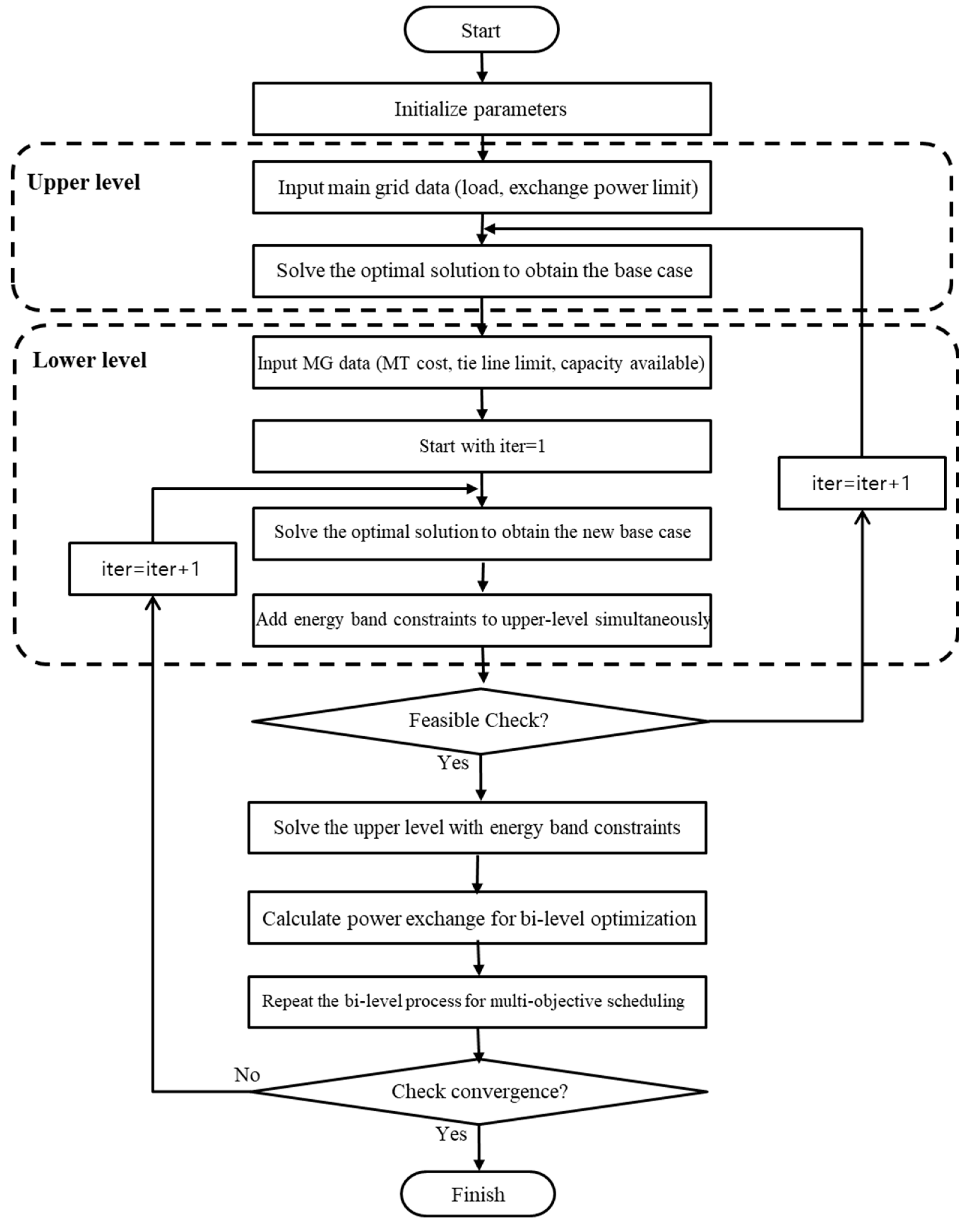
4.2. Solution Procedure

The bi-level optimization for cooperation between the DSO and MGO is implemented in the following sequential manner:

Step 1. Set the input parameters as well as the lower and upper limits of each power system variable for the bi-level optimization process.

Step 2. Choose the population size M, crossover and mutation probability, crossover and mutation index, and maximum number of generations.

Step 3. Solve the upper-level without the lower-level and obtain the initial base-case solution.

Step 4. After obtaining the base-case solution by solving the upper-level without any energy band constraints, solve the lower-level to determine the new base case. Here, the tie-line flow from the energy band between the DSO and MGO is taken as a decision variable, and this variable is returned to the upper-level.

Step 5. When violations are detected in the lower-level, solve the upper-level with all of the feedback information included, thereby creating a new base-case.

Step 6. Solve the lower-level in parallel with the new base-case.

Step 7. Repeat the bi-level process until the new base-case is established.

Step 8. If the multi-objective functions are to obtain the converged Pareto solution, the process terminates; otherwise, it is repeated from Step 3.

A flowchart of the detailed approach is presented in Figure 3.

5. Result and Discussion

5.1. Data

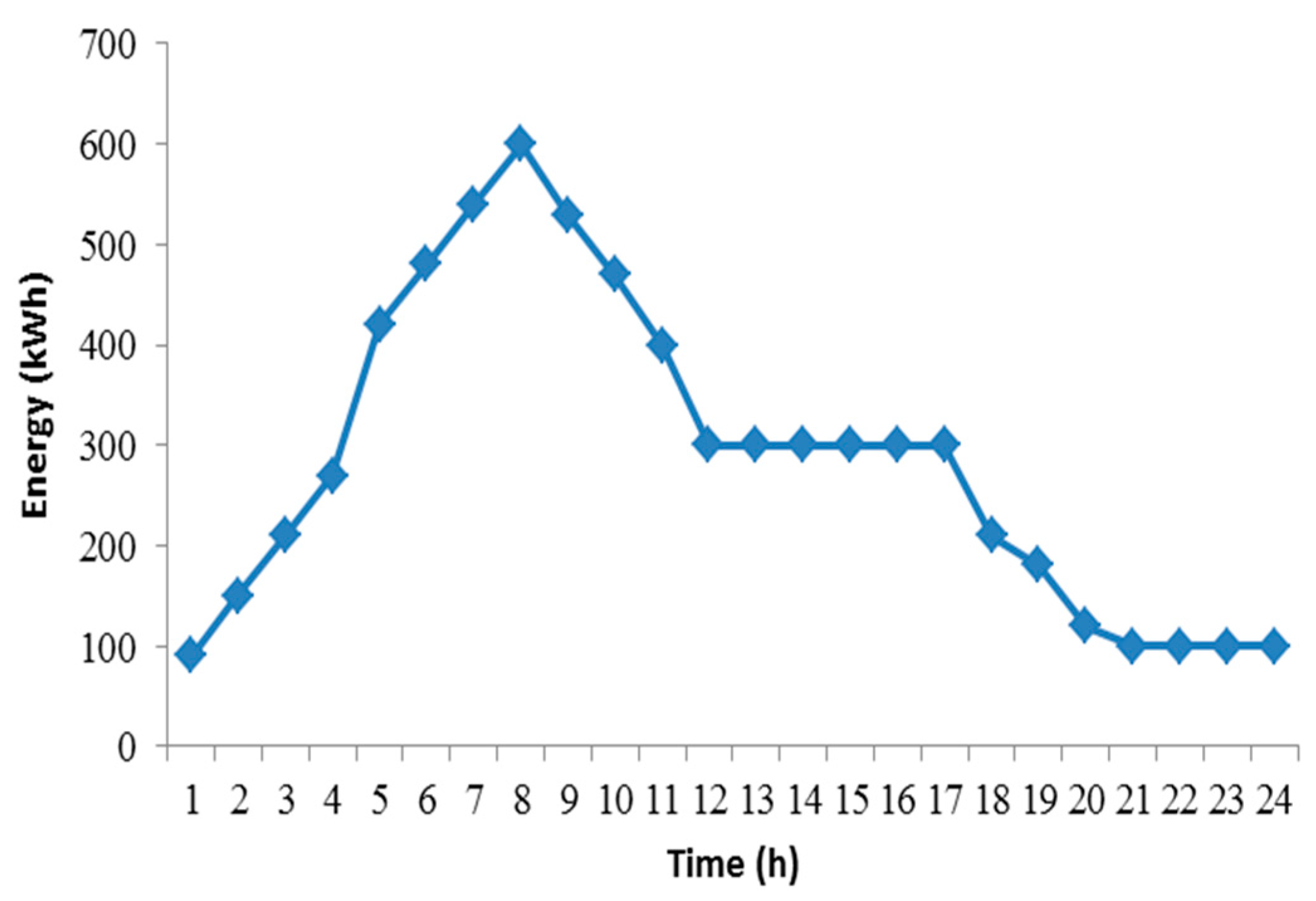
The MG contains distributed generation units, including WTs, MTs, and PV panels. The power for the WTs, PV panels, and total load were taken from [28], as shown in Figure 4. Since the load amount is greater than the total renewable energy at most times, other DER sources such as the MT and BESS are necessary to balance the MG demand. In this paper, we assume that the three types of loads (industrial, commercial, and residential customers) have a common characteristic and can be considered as critical and interruptible loads. Therefore, the three types of loads can be added together and considered the total load. Here, the total peak load is 500 kW. The MG structure is equipped with WT whose total installed capacity is 500 kW, PV 300 kW, and MT 500 kW.

In this study, the capacity of the BESS was 200 kWh, while the charging and discharging ramp-rate limits were both 50 kW/h. The battery efficiencies were 0.9 at any time step during the charging and discharging processes [32]. Furthermore, the renewable energy in the operating cost was assumed to have little effect on the final result. It was also assumed that no energy exchange occurred between MGs. All characteristics of the DERs and other values of the technical parameter are depicted in

Table 1. Values of technical parameters.

Parameter	Value	Parameter	Value
ρloss ($/kWh)	250	ρPVi ($/kWh)	11
PM,max (kW)	36	ρBESSi ($/kWh)	8
Pe,max (kW)	20	Vmin, Vmax (p.u.)	0.95, 1.05
ρmi ($/kWh)	71	PGmi,min, PGmi,max (kW)	0, 20
PWT,min,PWT,max (kW)	0, 250	PPV,min,PPV,max (kW)	0, 100

. Since we consider not only the scheduling in the MG, but also the operation of the tie-line, we assume that the minimum rated capacity of MT is set to zero in order to clarify the tie-line operation strategy considering the energy band. Figure 5 represents the forecasted real-time pricing (RTP) of the wholesale market and the retail market prices based on the time-of-use (TOU) scheme [33].

The residual energy curves of the BESS for a period of 24 h are shown in Figure 6. The initial state of charge of the BESS was 90 kWh. At 08:00, the BESS was fully charged. During the high-price period, the BESS injected power into the MG. Furthermore, at the end of the day, the residual energy of the BESS decreased to the initial value, which means that the energy of the BESS remained balanced throughout the day.

5.2. Simulation Results

To evaluate the superior performance of the proposed operation scheme, the following two cases were considered: Case 1: a bi-level optimization model that considers the tie-line flow without the energy band and Case 2: a bi-level optimization model that considers the tie-line flow within the energy band.

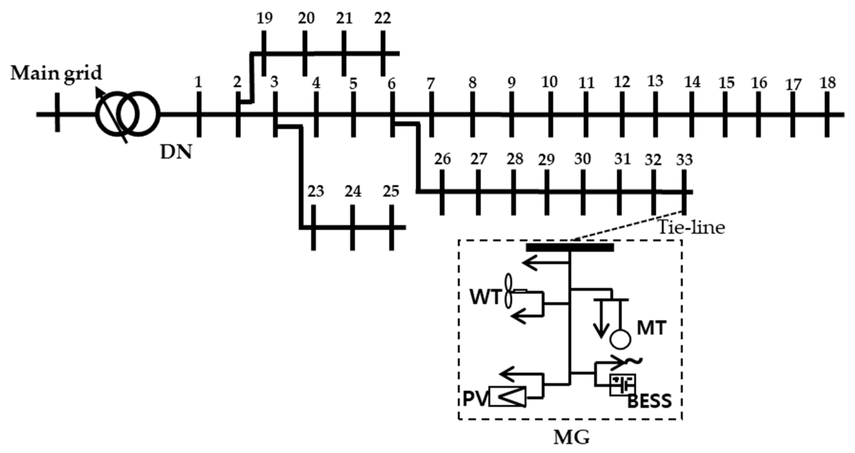
5.2.1. IEEE Test System

To demonstrate the validity of the proposed approach, an IEEE test system in which general European MGs [34] connected the modified IEEE 33-bus DN [35] was used for the simulation and analysis is shown in Figure 7. Details about the IEEE 33-bus DN can be found in [36]. The factors should be taken into account when modeling an MG integrated with the DN. Here, the MG was always connected to the DN by means of the tie-line. The maximum limit of the exchange power of the grid tie-line was 400 kW. The scheduling period was assumed to be a single day.

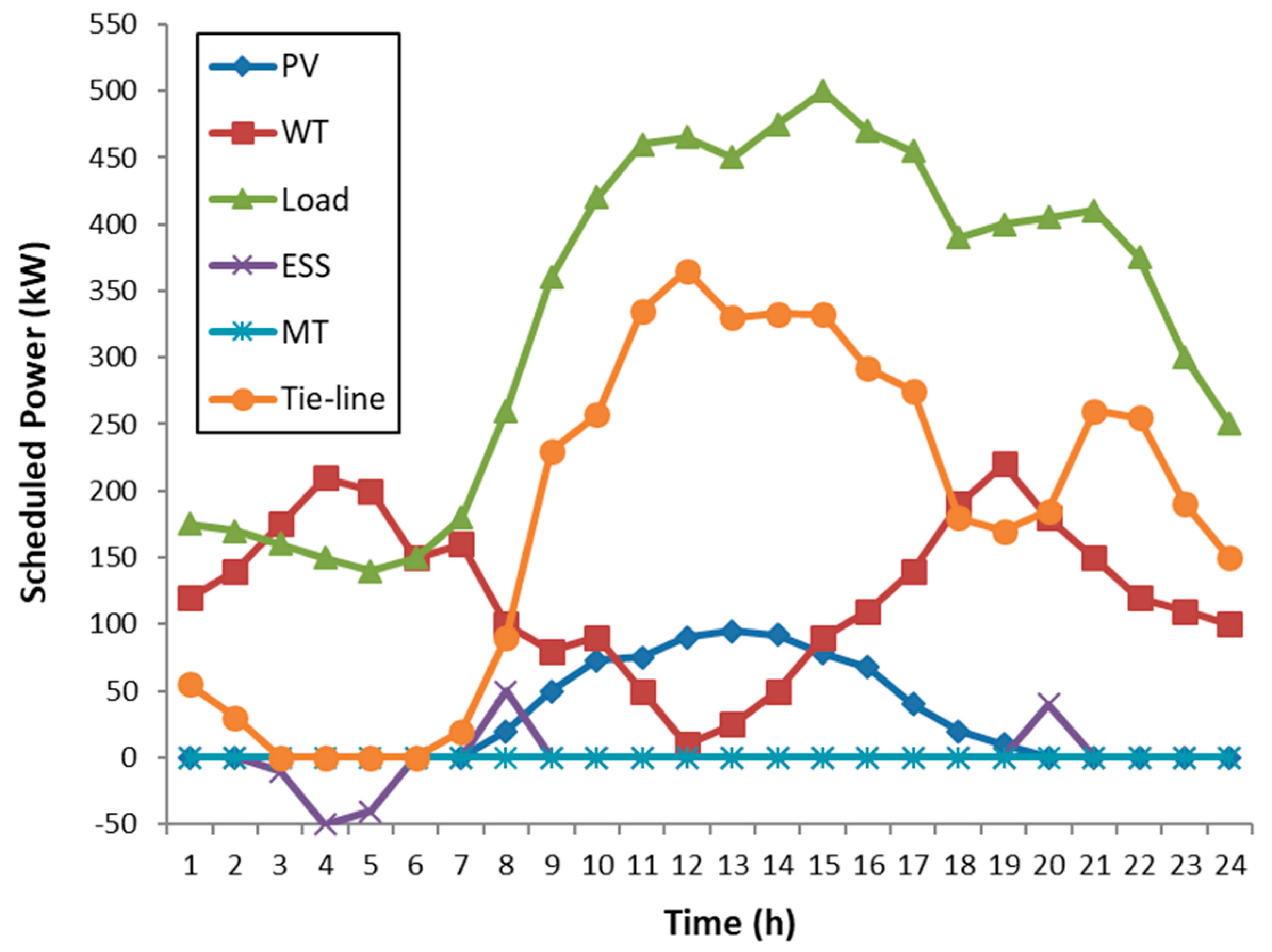
Figure 8 illustrates the resulting scheduled power scheme for the distributed units of the integrated MG, when the energy band was not considered, where the tie-line power accounted for the majority of the load. Moreover, the BESS charged and discharged less frequently. The batteries were charged from 02:00 to 04:00, while they were discharged at 07:00 and 19:00. Furthermore, the MG purchased energy from the DN to optimize the operational cost, because it was significantly lower than the MT cost. The manner in which the MGO shares the responsibility for ensuring balance of the supply and demand with the DSO under the fluctuating renewable energy depends on the operating condition of the tie-line flow.

The tie-line flow results of Case 1 are based on the predetermined (contractual) tie-line flow scenario. These results demonstrate that the MG rescheduled receiving the control signal from the DN for operating cost minimization with no tie-line constraints. Interestingly, the tie-line flow changed significantly to approximately 140 kW from 08:00 to 09:00, with a corresponding change in the load of 360 kW. Such substantial changes involve an increase in the potential risks or operational costs of the DN, even though this results in significant reductions in the operating costs of the MG. The important issue is the reduction of the reliability for the entire DN, which is far more significant than the minimization in the operating costs of the MG. This means that the scalability, namely the ability to incorporate MGs into the DN, may be restricted. In this case, fluctuations as large as 4334 kW could occur in the power transmission via the tie-line during the day.

We also evaluated the energy band operation scheme where the MG optimized the control signal of the tie-line flow within the energy band (Case 2). The sharing of reliability should be carefully considered when establishing the energy band size as an operational condition, owing to the trade-off between reliability and cost in the grid-connected system. We considered energy bands ranging from 30% to 80% and compared the results with those of Case 1, as indicated in

Table 2. Comparison of MG operational costs.

Time (h)	Contract (kW)	Scheduled Power (kW)
		(Energy Band)
		30%	40%	50%	60%	70%	80%
1	55	40.04	43.12	46.2	49.28	52.36	55.44
2	30	21.06	22.68	24.3	25.92	27.54	29.16
3	0	0	0	0	0	0	0
4	0	0	0	0	0	0	0
5	0	0	0	0	0	0	0
6	0	0	0	0	0	0	0
7	20	14.04	15.12	16.20	17.28	18.36	19.44
8	90	63.18	68.04	72.90	77.76	82.62	87.48
9	230	161.46	173.88	186.30	198.72	211.14	223.56
10	257	180.41	194.29	208.17	222.05	235.93	249.80
11	335	235.17	253.26	271.35	289.44	307.53	325.62
12	365	256.23	275.94	295.65	315.36	335.07	354.78
13	330	231.66	249.48	267.30	285.12	302.94	320.76
14	333	233.77	251.75	269.73	287.71	305.69	323.68
15	332	233.06	250.99	268.92	286.85	304.78	322.70
16	292	204.98	220.75	236.52	252.29	268.06	283.82
17	275	193.05	207.90	222.75	237.60	252.45	267.30
18	180	126.36	136.08	145.80	155.52	165.24	174.96
19	170	119.34	128.52	137.70	146.88	156.06	165.24
20	185	129.87	139.86	149.85	159.84	169.83	179.82
21	260	182.52	196.56	210.60	224.64	238.68	252.72
22	255	179.01	192.78	206.55	220.32	234.09	247.86
23	190	133.38	143.64	153.90	164.16	174.42	184.68
24	150	105.30	113.40	121.50	129.60	137.70	145.80
Ratio		70.23	75.64	81.04.	86.44	91.84	97.25

. According to the results, the ratio of the 80% energy band was almost equal to the contract power. In the proposed bi-level optimization model, ensuring the proposed ramping capability in the MG is essential for mitigating operational risks.

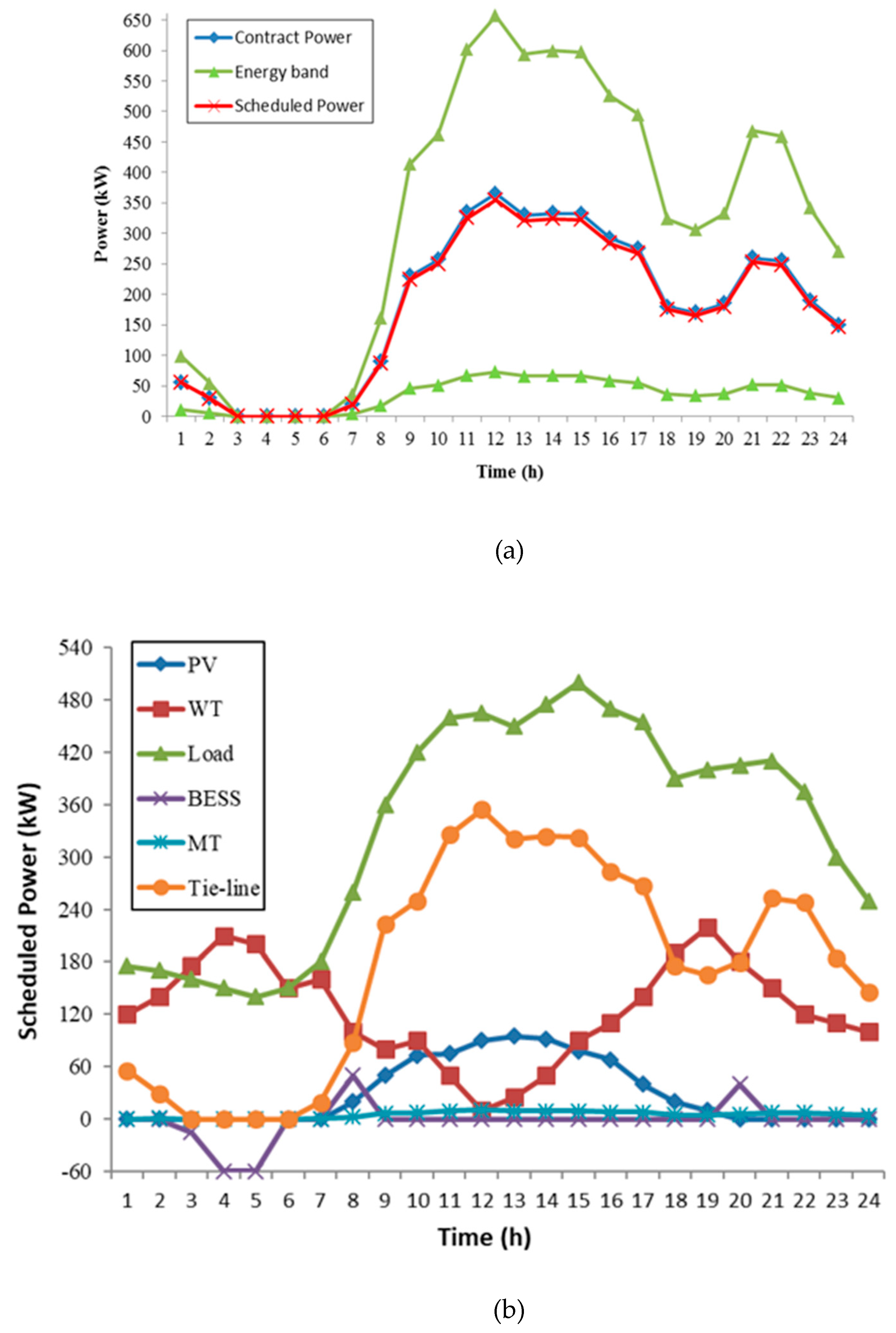
The scheduled power scheme for Case 2 with an energy band of 80% is plotted in Figure 9. It can be observed from Figure 9a that the scheduled power scheme was similar to the contract power. Limited control over the tie-line flow could cause the power system reliability of the MG to decrease owing to an increased supply–demand unbalance. As shown in Figure 9b, the BESS was charged for longer than that during Case 1 (from 03:00 to 05:00). The MT also generated power, which was used to ensure reliable operation between the DSO and MGO, because of the ramping capability of the proposed energy band scheme. Consequently, these results demonstrate that the increased responsibility for balancing the supply and demand requires preparation and planning to make sure that the MGO is capable of ramping.

Table 3. Comparison of the operational costs for each case.

Case	Operation Cost ($/h)		Note
	DSO	MGO
Base	856,374	519,482	No purchase of power from DN
Case 1	873,622	516,841	Purchase of power from DN through tie-line
Case 2	862,716	517.874	Purchase of power from DN with energy band of 80%

compares the operational costs of the DN for all of the cases. In the base case, that is, when no power was purchased from the DN, the operational cost was $519,482/h, while the operational costs for Cases 1 and 2 were $516,841/h and $517,212/h, respectively. Although the operational cost in the case of the proposed bi-level optimization model (Case 2) was 0.2% ($1033/h) higher than that for Case 1, it was 0.3% ($1608/h) lower than that for the base case. These results are relevant to the problems relating the MG operation; that is preventing shortages in the energy supply to the DN from worsening, even though the operational costs for both Case 2 and the base case were higher than that for Case 1.

To demonstrate the effectiveness of the bi-level optimization model for cooperation between the DSO and MGO, the following two scenarios of Case 2 were considered: Scenario A: no bi-level optimization model with Case 2, and Scenario B: bi-level optimization model with Case 2.

Table 4. Comparison of operational costs for scenarios in Case 2.

Scenario	Operation Cost ($/h)		Note
	DSO	MGO
Scenario A	864,274	512,638	No bi-level model with Case 2
Scenario B	862,716	517,874	Proposed bi-level model with Case 2

presents a comparison of the operational costs for each scenario in Case 2. In Scenario A, the MG purchased power from the wholesale market at the RTP, because the feedback information including the operational costs of MG and energy band, was not considered. According to the comparison results, the operational cost of the MG in Scenario A was $512,638/h, which was lower than that in Scenario B, namely $517,874/h, but the operational cost of the DN in Scenario A was higher than that in Scenario B.

The optimal results of the proposed approach for each case are summarized in

Table 5. Comparison of the optimal results for each case.

Case	Operational Cost (DSO)	Profit (MGO)
Case 1	873,622	747,216
Case 2	862,716	746,085

. Comparing the operation cost of the DSO, Case 2 was lower than Case 1, while the MGO profit in Case 2 was lower than Case 1. It can be observed that the DSO operational cost was the lowest, even though the MGO profit was little reduced in Case 2. Therefore, the results indicated in our study confirm that the proposed approach provides the DSO and MGO with the optimal solution for reliable and economical operation.

5.2.2. Actual Power System

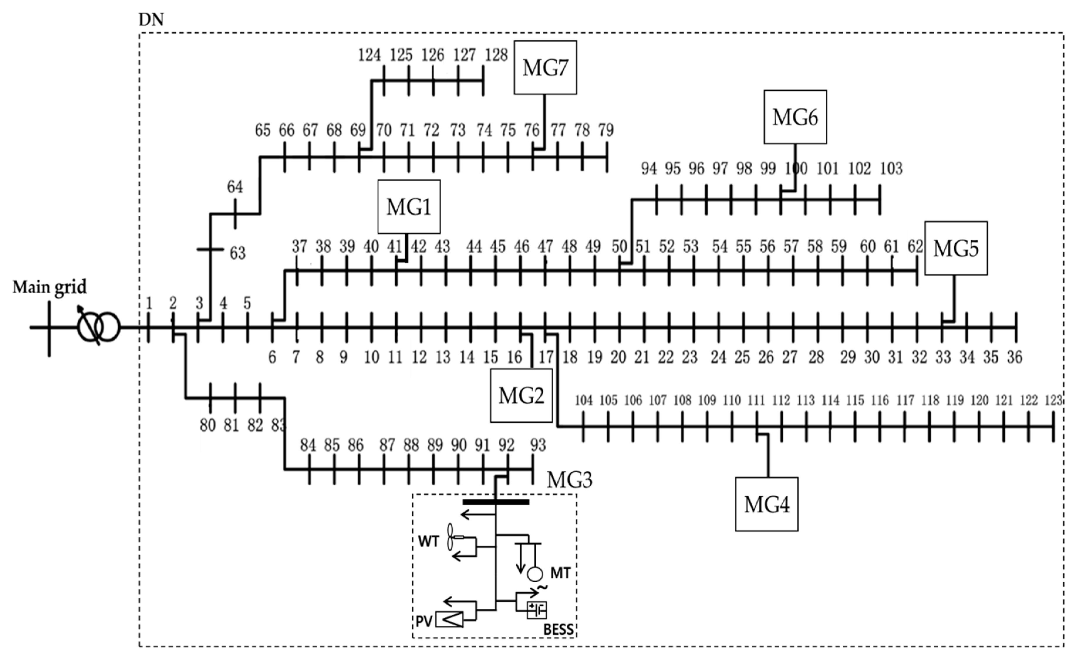
We evaluated the practical applicability of the proposed approach for large-scale power systems, by applying the results of our work to an actual power system in Shandong, China, called the Changdao project [37], consisting of 128 buses and 7 MGs as shown in Figure 10. All of the MGs were constantly connected to the DN by means of a single tie-line. The maximum limit of the tie-line flow was 1000 kW. The scheduling period was considered to be a single day. The data for every MG and the capacity parameters were listed in

Table 6. Capacity parameters.

Type	Minimum Power (kW)	Maximum Power (kW)	Number of Units	Ramp up/down Rate (kW/min)
MT	0	1000	11	500/400
WT	0	1000	11	-
PV	0	1500	10	-
ESS	−1500	1500	7	-

.

The scheduled power scheme for Case 2 with an energy band of 60% is shown in Figure 11. As can be seen from Figure 11b, the BESS was charged for longer, from 04:00 to 07:00, than in Case 1, with the MTs also generating additional power. These results indicate that the proposed bi-level optimization model with the energy band can effectively improve reliable operations between the DSO and MGO.

Table 7. Comparison of operational costs for each case.

Case	Operation Cost ($/h)		Note
	DSO	MGO
Base	2,081,643	1,454,549	No purchase of power from DN
Case 1	2,548,231	1,447,154	Purchase of power from DN through tie-line
Case 2	2,320,075	1,450,047	Purchase of power from DN within energy band of 60%

compares the operational costs for each case. In the base case, the operational cost was $1,454,549/h when no power was purchased from the DN. In comparison, the operational costs for Cases 1 and 2 were $1,447,154/h and $1,450,047/h, respectively. Although the operational cost for the proposed scheme (Case 2) was 0.2% ($2893/h) higher than that for Case 1, it was lower than that for the case in which no power was purchased from the DN by approximately 0.3% ($4532/h). Therefore, the proposed bi-level optimization model based on a 60% energy band provides superior balance for economical and reliable operation between the DSO and MGO.

Table 8. Comparison of operational costs for each Scenario in Case 2.

Scenario	Operation Cost ($/h)		Note
	DSO	MGO
Scenario A	2,527,983	1,387,562	No bi-level model with Case 2
Scenario B	2,320,075	1,450,047	Proposed bi-level model with Case 2

presented a comparison of the operational costs for each scenario in Case 2. To confirm the results, we assumed the same scenario as in the IEEE test system described previously. According to the comparison results, the MG operational cost for Scenario A was $1,387,562/h, which was lower than that for Scenario B, namely $1,450,047/h, but the operational cost of the DSO for Scenario A is higher than that for Scenario B. It can be observed that the proposed bi-level model can reduce the DSO operational cost although the MGO operational cost increases, because the MG operational cost can be reduced by the proposed tie-line control strategy.

Table 9. Comparison optimal results for each case.

Case	Operational Cost (DSO)	Profit (MGO)
Case 1	2,548,231	988,274
Case 2	2,320,075	980,610

displayed the optimal results of the proposed approach for each case. Similar to the result for the IEEE test system previously, the operation cost of the DSO in Case 2 was lower than Case 1, while the MGO profit in Case 2 was lower than Case 1. It can be seen that the DSO operational cost was the lowest, even though the MGO profit was little reduced in Case 2. Therefore, it should be noted that the proposed approach provides the optimal balance for reliable and economical operation between the DSO and MGO.

5.3. Performance Test

The multi-objective performance of the MNSGA-II was evaluated by comparing the Pareto solutions obtained using the NSGA-II and MNSGA-II for 30 simulations performed on both the IEEE test system and actual power system. The convergence metric, spread/diversity metric, inverted generational distance, and minimum spacing metric were calculated for the non-dominated solutions obtained using the NSGA-II and MNSGA-II [38]. A total of 30 independent trials were conducted to select the appropriate values for these parameters and the optimal parameters selected are presented in

Table 10. Parameters used for non-dominated sorting genetic algorithm II (NSGA-II) and modified version of the NSGA-II (MNSGA-II).

Parameter	IEEE Test System		Actual Power System
	NSGA-II	MNSGA-II	NSGA-II	MNSGA-II
Population size	100	100	200	200
Max. no. of generations	30	30	30	30
Crossover probability	0.8	0.8	0.9	0.9
Mutation probability	1/12	1/12	1/75	1/75
Crossover index	1	1	2	2
Mutation index	10	10	20	20

. In this case, the initial weight factor, w, was set to 0.5.

Figure 12 displays the optimization results of the Pareto solution obtained in Case 2 among the particle swarm optimization (PSO) [39], adaptive modified PSO (AMPSO) [40], strength Pareto evolutionary algorithm (SPEA) [41], genetic algorithm (GA) [42], NSGA-II [43], and MNSGA-II on the test system and actual system. Note that the third point converged as the Pareto solution in the case of MNSGA-II for both systems.

Table 11. Comparison result of different algorithms for Case 2.

Test System	Algorithm	DSO Operating Cost ($/h)	MGO Profit ($/h)	Total Run Time (min)
IEEE test system	PSO	869,694	749,964	6.27
	AMPSO	866,047	749,165	1.95
	SPEA	865,147	750,132	2.03
	GA	870,486	750,641	5.83
	NSGA-II	863,208	746,927	8.54
	MNSGA-II	862,716	746,085	1.83
Actual power system	PSO	2,339,648	994,648	22.74
	AMPSO	2,325,348	985,912	8.97
	SPEA	2,328,321	984,315	10.84
	GA	2,341,934	997,324	21.25
	NSGA-II	2,322,496	981,073	24.31.
	MNSGA-II	2,320,075	980,610	5.46

indicates the comparison results for each system. According to the comparison results, it is clear that the DSO operating cost and MGO profit were lower in the proposed MNSGA-II than in the other algorithms for both systems. These results may be small in terms of the overall operation, but a value is not small in terms of the cost regarding the margin of the tie-line between the DN and MG for sharing the exchange information. As shown in Table 11, the run time of the proposed approach was significantly reduced compared to the others, particularly for large power systems, owing to the parallel processing based on the bi-level model. These results demonstrate that the proposed approach is suitable for the requirements of realistic power system operation.

The superior performance of the optimization process for multi-objective problem obtained Pareto-fronts between DSO and MGO using the MNSGA-II are shown in Figure 13. As shown in Figure 13a, when the weighting factors were w_u = 0.3 (upper-level) and w_l = 0.7 (lower-level), the convergence points of the Pareto-front for profit and operating cost in the IEEE test system were obtained after the 21th iterative cycle. On the other hand, when the weighting factors were w_u = 0.4 and w_l = 0.6, the Pareto-front converged after the 28th iterative cycle (see Figure 13b). On the basis of the results in Figure 13, it can be concluded that the performance of multi-objective optimization was superior, as it exhibited higher convergence speed and required fewer iterative cycles to converge. Therefore, the proposed approach results in optimal operational solutions and can assist in decision-making whenever there is a trade-off between the DSO and MGO in power systems.

6. Conclusions

A bi-level operation model based on the energy band has been proposed for improved cooperation. The upper-level model describes the optimal dispatch of the DN with the aim of minimizing the operating cost. The lower-level model considers the scheduling information obtained by the upper-level for feedback information as the objective for maximizing the MG profit for cooperation between the DSO and MGO. In our work, instead of converting the bi-level optimization problem into a single level, a multi-objective optimization problem relating to the cooperation between the DSO and MGO was presented, in which the MNSGA-II was used to solve the proposed model, and applied to the cooperation of the variable relationships between the DSO and MGO. Owing to the trade-off between the stable operation of the DN and economical operation of the MG, the DSO and MGO cautiously consider the “Pareto solution” to solve the multi-objective problem with bi-level optimization while improving the operations of the entire system. The simulation results demonstrated that when an MG is integrated into the DN, the benefits of the entire system are optimized. During the simulations, by using this approach, the tie-line flow could be managed smoothly within the energy band, although the results for the grid-connected MG operation-related approach showed that the tie-line flow changes sharply. Therefore, the proposed optimization approach provides additional economic benefits for power systems, along with performance improvements and increased reliability for cooperation between the DSO and MGO. Our future work will focus on the reasonable selection of additional energy band values while considering various factors as well as the tie-line flow.

References

- Kim, H.Y.; Kim, M.K. Optimal generation rescheduling for meshed AC/HIS grids with multi-terminal voltage source converter high voltage direct current and battery energy storage system. Energy 2017, 119, 309–321. [Google Scholar] [CrossRef]
- Sheikhahmadi, P.; Mafakheri, R.; Bahramara, S.; Damavandi, M.Y.; Catalao, J. Risk-based two-stage stochastic optimization problem of micro-grid operation with renewables and incentive based demand response programs. Energies 2018, 11, 610. [Google Scholar] [CrossRef]
- Zamora, R.; Srivastava, A.K. Controls for microgrids with storage review, challenges, and research needs. Renew. Sustain. Energy Rev. 2010, 14, 2009–2018. [Google Scholar] [CrossRef]
- Shi, L.; Luo, Y.; Gy, T. Bidding strategy of microgrid with consideration of uncertainty for participating in power market. Int. J. Electr. Power Energy Syst. 2014, 59, 1–13. [Google Scholar] [CrossRef]
- Feijoo, F.; Das, T.K. Emissions control via carbon policies and microgrid generation: A bilevel model and pareto analysis. Energy 2015, 90, 1545–1555. [Google Scholar] [CrossRef]
- Kim, D.; Kwon, H.G.; Kim, M.K.; Park, J.K.; Park, H.G. Determining the flexible ramping capacity of electric vehicles to enhance locational flexibility. Energies 2017, 10, 2028. [Google Scholar] [CrossRef]
- Erdine, O. Economic impacts of small-scale own generating and storage units, and electric vehicles under different demand response strategies for smart households. Appl. Energy 2014, 126, 142–150. [Google Scholar] [CrossRef]
- Akorede, M.F.; Hizam, H.; Pouresmaeil, E. Distributed energy resources and benefits to the environment. Renew. Sustain. Energy Rev. 2010, 14, 724–734. [Google Scholar] [CrossRef]
- Talari, S.; Khah, M.S.; Osorio, G.; Aghael, J. Stochastic modeliling of renewable energy sources from operatiors’ point of view: A survey. Renew. Sustain. Energy Rev. 2017, 81, 1953–1965. [Google Scholar] [CrossRef]
- Kou, P.; Feng, Y.; Liang, D.; Gao, L. A model predictive control approach for matching uncertain wind generation with PEV charging demand in a microgrid. Int. J. Electr. Power Energy Syst. 2019, 105, 488–499. [Google Scholar] [CrossRef]
- Rist, J.F.; Dias, M.F.; Palman, M.; Zelazo, D.; Cukurel, B. Economic dispatch of a single micro-gas turbine under CHP operation. Appl. Energy 2017, 200, 1–18. [Google Scholar] [CrossRef]
- Velik, R.; Nicolay, P. Grid price dependent energy management in microgrid using a modified simulated annealing triple optimizer. Appl. Energy 2014, 130, 384–395. [Google Scholar] [CrossRef]
- Palizban, O.; Kauhaniemi, K.; Guerrero, J.M. Microgrids in active network management—Part II: System operation, power quality and protection. Renew. Sustain. Energy Rev. 2014, 36, 440–451. [Google Scholar] [CrossRef]
- Sechilariu, M.; Wang, B.C.; Locment, F.; Jouglet, A. DC microgrid power flow optimization by multi-layer supervision control, design and experimental validation. Energy Convers. Manag. 2014, 82, 1–10. [Google Scholar] [CrossRef]
- Sechilariu, M.; Wang, B.C.; Locment, F. Supervision control for optimal energy cost management in DC microgrid: Design and simulation. Int. J. Electr. Power Energy Syst. 2014, 58, 140–149. [Google Scholar] [CrossRef]
- Li, T.S.; Zhang, H.G.; Huang, B.N.; Teng, F. Distributed optimal economic dispatch based on multi-agent system framework in combined heat and power systems. Appl. Sci. 2016, 6, 308. [Google Scholar] [CrossRef]
- Jiang, Q.; Xue, M.; Geng, G. Energy management of microgrid in grid connected and stand-alone modes. IEEE Trans. Power Syst. 2013, 28, 3380–3389. [Google Scholar] [CrossRef]
- Liu, G.; Mahmoudi, N.; Chen, K. Microgrids real-time pricing based on clustering techniques. Energies 2018, 11, 1388. [Google Scholar] [CrossRef]
- Tan, S.; Xu, J.; Panda, S.K. Optimization of distribution network incorporating distributed generators: An integrated approach. IEEE Trans. Power Syst. 2013, 28, 2421–2432. [Google Scholar] [CrossRef]
- Khodaei, A.; Shahidehpour, M. Microgrid-based co-optimization of generation and transmission planning in power systems. IEEE Trans. Power Syst. 2013, 28, 1582–1590. [Google Scholar] [CrossRef]
- Zenginis, I.; Vardakas, J.S.; Echave, C.; Morato, M.; Abadal, J. Cooperation in microgrids through power exchange: An optimal sizing and operation approach. Appl. Sci. 2017, 203, 972. [Google Scholar] [CrossRef]
- Bahramara, S.; Moghaddam, M.P.; Haghifam, M.R. A bi-level optimization model for operation of distribution networks with micro grids. Int. J. Electr. Power Energy Syst. 2016, 82, 169–178. [Google Scholar] [CrossRef]
- Shi, N.; Luo, Y. Bi-level programming approach for the optimal allocation of energy storage systems in distribution networks. Appl. Sci. 2017, 7, 398. [Google Scholar] [CrossRef]
- Xie, J.; Zhong, J.; Li, Z.; Gan, D. Environmental economic unit commitment using mixed integer linear programming. Eur. Trans. Electr. Power 2011, 21, 772–786. [Google Scholar] [CrossRef]
- Muthuswamy, R.; Krishnan, M.; Subramanian, K.; Subramanian, B. Environmental and economic power dispatch of thermal generators using modified NSGA-II algorithm. Int. Trans. Electr. Energy Syst. 2014, 25, 1552–1569. [Google Scholar] [CrossRef]
- Lee, S.Y.; Jin, Y.G.; Yoon, Y.T. Determining the optimal reserve capacity in a microgrid with islanded operation. IEEE Trans. Power Syst. 2016, 31, 1369–1376. [Google Scholar] [CrossRef]
- Colson, B.; Marcotte, P.; Savard, G. An overview of bilevel optimization. Ann. Oper. Res. 2007, 153, 235–256. [Google Scholar] [CrossRef]
- Liu, Y.; Jiang, C.; Shen, J.; Zhou, X. Energy management for grid-connected micro grid with renewable energies and dispatched loads. Prz. Elektrotechniczny Electr. Rev. 2012, 88, 87–93. [Google Scholar]
- Mazidi, M.; Zakariazadeh, A.; Jadid, S.; Siano, P. Integrated scheduling of renewable generation and demand response programs in a microgrid. Energy Conv. Manag. 2014, 86, 1118–1127. [Google Scholar] [CrossRef]
- Deb, K. Multi-Objective Optimization Using Evolutionary Algorithms; Wiley: Chichester, UK, 2001. [Google Scholar]
- Luo, B.; Zheng, J.; Xie, J.; Wu, J. Dynamic crowding distance—A new diversity maintenance strategy for MOEAs. In Proceedings of the IEEE International Conference on Natural Computation, Jinan, China, 18–20 October 2008; pp. 580–585. [Google Scholar]
- Mingrui, Z.; Jie, C.; Zhichao, D.; Shaobo, W.; Hua, S. Economic operation of microgrid considering regulation of interactive power. Chin. Soc. Electr. Eng. 2014, 34, 1013–1023. [Google Scholar]
- Sahedi, M.M.; Duki, E.A.; Kia, M. Simultanous emergency demand response programming and unit commitment programming in comparison with interruptible load contracts. IET Gener. Transm. Distrib. 2012, 6, 605–611. [Google Scholar]
- Papathanassiou, S.; Hatziargyrlou, N.D.; Strunz, K. A benchmark low voltage microgrid for steady state and transient analysis. In Proceedings of the CIGRE Symposium: Power Systems with Dispersed Generation, Athens, Greek, April 2005. [Google Scholar]
- Wang, Z.; Chen, B.; Wang, J.; Begovic, M.; Chen, C. Coordinated energy management of networked microgrids in distribution systems. IEEE Trans. Smart Grid 2015, 6, 45–53. [Google Scholar] [CrossRef]
- Baran, M.E.; Wu, F.F. Network reconfiguration in distribution systems for loss reduction and load balancing. IEEE Trans. Power Deliv. 1989, 4, 1401–1407. [Google Scholar] [CrossRef]
- Project 1090: Shangdong Changdao 27.2 MW Wind Power Project 2008. Available online: https://cdm.unfccc.int/Projects/DB/DNV-CUK1176964325.8/view (accessed on 21 January 2008).
- Kim, H.Y.; Kim, M.K.; Kim, S. Multi-objective scheduling optimization based on a modified non-dominated sorting genetic algorithm-II in voltage source converter multi-terminal high voltage dc grid connected offshore wind farms with battery energy storage systems. Energies 2017, 10, 986. [Google Scholar] [CrossRef]
- Mondai, D.; Chakrabarti, A.; Sengupta, A. Optimal placement and parameter setting of SVC and TCSC using PSO to mitigate small signal stability problem. Int. J. Electr. Power Energy Syst. 2012, 42, 334–340. [Google Scholar] [CrossRef]
- Moghaddam, A.A.; Seifi, A.; Niknam, T.; Pahlavani, A.R.A. Multi-objective operation management of a renewable MG with back-up micro-turbine/fuel cell/battery hybrid power source. Energy 2011, 36, 6490–6507. [Google Scholar] [CrossRef]
- Yuan, X.; Zhang, B.; Wang, P.; Liang, J.; Yuan, Y.; Huang, Y.; Lei, X. Multi-objective optimal power flow based on improved strength Pareto evolutionary algorithm. Energy 2017, 122, 70–82. [Google Scholar] [CrossRef]
- Gerbex, S.; Cherkaoui, R.; Germond, A.J. Optimal location of multi-type FACTS devices in a power system by means of Genetic Algorithms. IEEE Trans. Power Syst. 2001, 16, 537–544. [Google Scholar] [CrossRef]
- Marouani, I.; Guesmi, T.; Abdallah, H.H.; Ouali, A. Application of NSGA-II approach to optimal location of UPFC devices in electrical power systems. J. Sci. Res. 2011, 10, 592–603. [Google Scholar]
Figure 1.
Energy band operational scheme.
Figure 2.
Overall scheme of a bi-level model. MGO: microgrid operator; DSO: distribution network operator; WT: wind turbine; PV: photovoltaic; MT: microturbine; BESS: battery energy storage system.
Figure 3.
Bi-level optimization process.
Figure 4.
Forecasting power of PV panels and WTs and load for test system.
Figure 5.
Market price information.
Figure 6.
Residual energy of BESS.
Figure 7.
IEEE (Institute of Electrical and Electronics Engineers) test system.
Figure 8.
Scheduled power scheme for distributed units for Case 1.
Figure 9.
Scheduled power scheme for Case 2 for energy band of 80%: (a) Results for energy band, (b) Scheduled power volumes for distributed units.
Figure 10.
Actual power system in China.
Figure 11.
Scheduled power scheme for Case 2 within energy band of 60%: (a) Results for energy band, (b) Scheduled power volumes for distributed units.
Figure 12.
Optimization results for each system. PSO: particle swarm optimization; adaptive modified PSO; SPEA: strength Pareto evolutionary algorithm; GA: strength Pareto evolutionary algorithm; NSGA-II: non-dominated sorting genetic algorithm II; MNSGA-II: modified version of the non-dominated sorting genetic algorithm II: (a) IEEE test system, (b) Actual power system.
Figure 13.
Optimization process for obtained Pareto-front via MNSGA-II: (a) IEEE test system, (b) Actual power system.