Resonance Instability of Photovoltaic E-Bike Charging Stations: Control Parameters Analysis, Modeling and Experiment

Abstract

This article presents an in-situ comparative analysis and power quality tests of a newly developed photovoltaic charging system for e-bikes. The various control methods of the inverter are modeled and a single-phase grid-connected inverter is tested under different conditions. Models are constituted for two current control methods; the proportional resonance and the synchronous rotating frames. In order to determine the influence of the control parameters, the system is analyzed analytically in the time domain as well as in the frequency domain by simulation. The tests indicated the resonance instability of the photovoltaic inverter. The passivity impedance-based stability criterion is applied in order to analyze the phenomenon of resonance instability. In conclusion, the phase-locked loop (PLL) bandwidth and control parameters of the current loop have a major effect on the output admittance of the inverter, which should be adjusted to make the system stable.

1. Introduction

Transportation takes up a lot of space on the overall energy spending of the population. The future transmission capacity of the grid might be limited because of the increasing electricity demand, therefore electric mobility of the future would aim to be less demanding for the grid [1]. Due to the optimization of the space utilization of rooftop photovoltaic systems and charging stations, photovoltaic (PV) electric vehicle (EV) charging stations [2,3] and photovoltaic electric bicycle charging stations [4,5] have received widespread attention [6]. Since photovoltaic charging stations require sufficient sunshine time and parking space, they are generally far from buildings [7]. Therefore, the photovoltaic charging station is often at the end of the low-voltage power grid of the building, and the grid impedance has a great influence on the stable operation of the photovoltaic charging station [8]. To improve the performance of new forms of EV charging such as by solar energy, it would be interesting to evaluate and quantify the power quality of charging stations.

The common stability analysis methods of grid-connected inverters are the state space method [9] and the impedance analysis method [10]. When applying the state space method for stability analysis, all parameters of the inverter and the grid must be acquired to establish the state space model [11]. Due to the curse of dimensionality problem [12], the state space method is very complicated for the analysis process of a large-scale grid-connected inverter-grid system.

Therefore, the impedance analysis method is proposed [13]. This method considers the inverter and grid system as two independent subsystems and establishes an impedance model separately or directly measures the impedance by the frequency sweeping method. Then, through the Nyquist criterion, whether the inverter-grid system is stable or not can be judged. In this article, the passivity impedance-based stability criterion [14] and the impedance analysis method are combined to analyze the undesired resonance or harmonic phenomenon, which is called resonance instability [15,16].

In Section 2, the power quality of a photovoltaic (PV) charging station for e-bikes at the campus of the University of Twente (UT) [17] is measured and analyzed. This grid-connected PV charging station has been developed in house by UT using commercially available components (275 W_p of Canadian Solar^® PV modules and 2.0 kW inverter SOLAX Power^® X1 Series) and was installed by the end of 2017.

The resonance instability due to the grid impedance is found in the experimental results. The phenomenon of resonance instability, its principles, and its stability criteria are discussed. In Section 3, two common single-phase photovoltaic inverter control methods are presented as models. The modeling considers the influence of the phase-locked loop (PLL) on the inverter impedance. In Section 4, the model that is presented in Section 3 is validated through simulation. In the simulation, the phenomenon of resonance instability in the experiment is reproduced. In Section 5, the influences of various parameters on the stability of the inverter in each frequency band are analyzed and discussed. In addition, the improvement methods are presented and validated through simulation. The paper ends with conclusions in Section 6.

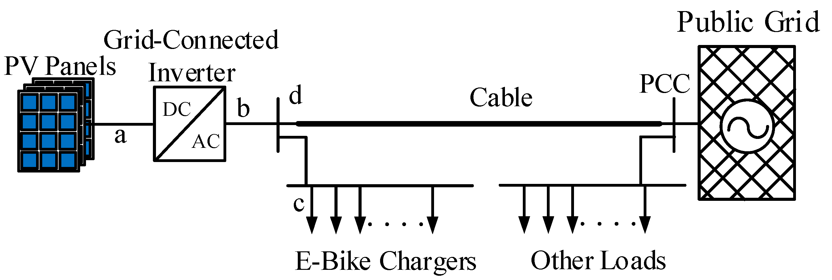
2. Experimental Study

2.1. Experimental Set-Up

The PV charging station for e-bikes is located in the bicycle parking lot of a central building in the UT Campus, enabling the public to charge their e-bikes with solar energy. Figure 1 shows the PV charging station with six dark mono-crystalline silicon PV modules of Canadian Solar^® ALL-BLACK CS6K-275 (marked with red dotted squares at the upper part of Figure 1), and a single-phase grid-connected inverter with a rated power of 2 kW (at left part of Figure 1). For further details on the PV modules and the inverter, please refer to References [18,19], respectively. One can also see in Figure 1, the flexible CIGS mini modules in the front wheel PV of the solar e-bikes.

The single-line diagram of the photovoltaic charging station is illustrated in Figure 2. As shown in Figure 2, six photovoltaic panels are connected to the DC side of the grid-connected inverter. The AC side of the inverter is connected to the public at the point of common coupling (PCC), so that the charging may be effectuated from the grid when there is no solar input. The PCC is located on the secondary side of the transformer of the building in Figure 1. The electrical distance between the inverter (point b) and PCC is relatively long, and there are also many non-linear loads that are switched at any time in the building. These together make the grid-connected inverter connected to a time-varying weak grid.

In order to analyze the power quality of the photovoltaic charging station, current and voltage sensors were installed in point a (DC bus), b (inverter output), c (local load) and d (grid) of Figure 2.

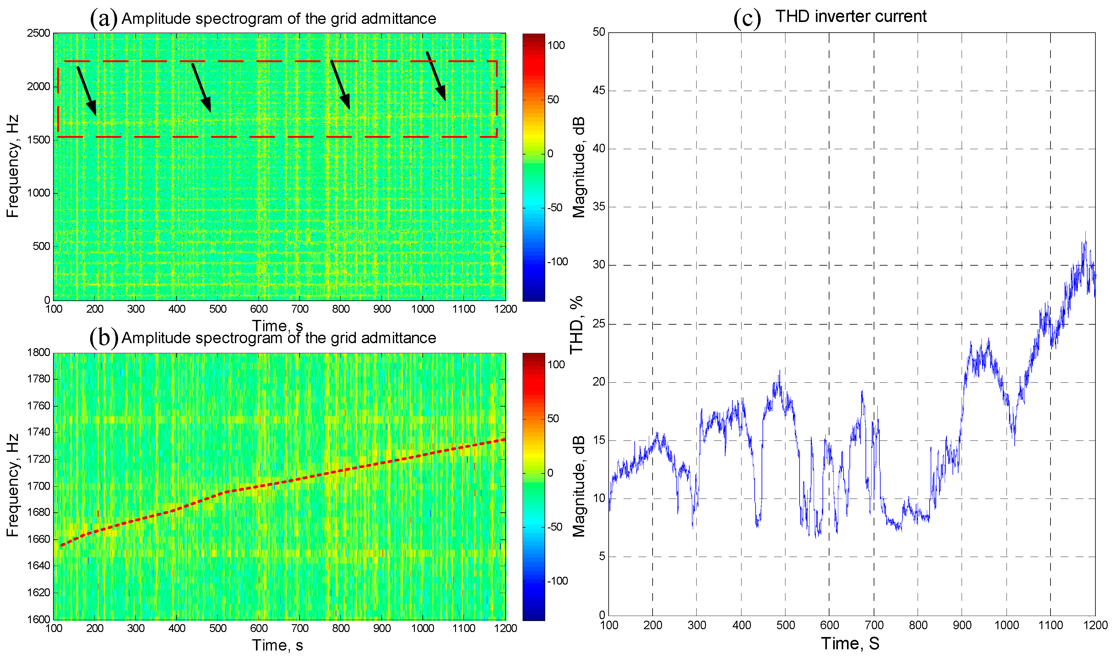
2.2. Experimental Results

In one test case, when the inverter output power and the power of local load (point c in Figure 2) did not change significantly, the total harmonic distortion (THD) of the inverter output current abnormally rose, as shown in Figure 3c.

By using the passive line impedance estimation method [20,21], the grid admittance amplitude spectrogram is obtained from the grid voltage and current information, as shown in Figure 3a. Its partial enlargement is shown in Figure 3b. In Figure 3a,b, the abscissa represents time, the ordinate represents frequency, and the color in the figure represents the amplitude (dB) of the grid admittance, with warm colors representing larger amplitudes and cool colors representing smaller amplitudes.

As shown in the red dotted square, indicated by the black arrow in Figure 3a, there was a resonance component of grid admittance with about a 10 dB amplitude rising from 1650 Hz to 1730 Hz. It passed through 1730 Hz from below at around 1000 s (see the partial enlargement (Figure 3b) for a clearer view). The THD of the inverter output current also started to increase around t = 1000 s (Figure 3c). This may be caused by a change in the operating state of other loads in the grid.

The undesired increasing of the THD of the inverter output current can lead to increased copper losses and a shortened life of the transformer, and it can also cause relay protection equipment to malfunction. If the THD continues to increase, it will also cause the inverter to lose stability and stop operation.

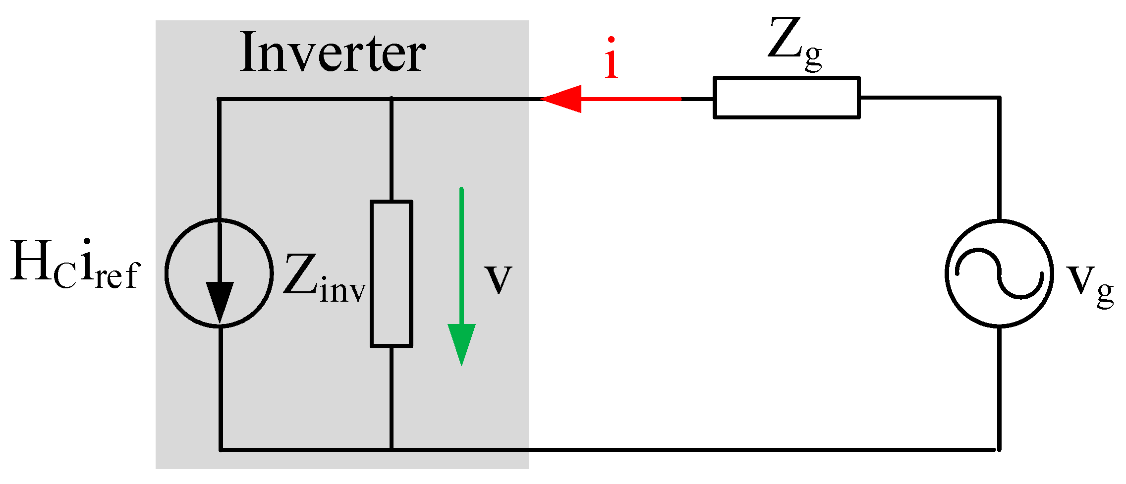
2.3. Passivity Impedance-Based Stability Criterion

Similar phenomena were also described in Reference [22], and called “resonance instability” or “harmonic instability”. This can be explained by the impedance-based stability criterion [13] and passivity theory [14]. Considering the nonlinearity of an inverter-grid system, the linearization of the equivalent circuit is based on the small signal modeling, as illustrated in Figure 4.

Most grid-connected inverters use the current tracking mode, so the inverter can be thought of as an ideal current source (H_ci_ref) and an inverter output impedance (Z_inv) connected in parallel, as shown in Figure 4, in the grey box.

The expression of the inverter output current is expressed in Equation (1).

$$\mathrm{i}={\mathrm{H}}_{\mathrm{C}}\left(\mathrm{s}\right){\mathrm{i}}_{\mathrm{ref}}+{\mathrm{Y}}_{\mathrm{inv}}\left(\mathrm{s}\right)\mathrm{v}$$

(1)

where i is the inverter output current; H_c(s) is the transfer function of the current control loop of the inverter; i_ref is the reference current; Y_inv(s) is the inverter output admittance and v is the inverter output voltage.

The complete inverter output current expression of the inverter-grid system is obtained in Equation (2), by Equation (1) and Figure 4,

$$\mathrm{i}=\underset{\mathrm{H}\left(\mathrm{s}\right)}{\underbrace{\frac{{\mathrm{H}}_{\mathrm{C}}\left(\mathrm{s}\right)}{1+Y_{\mathrm{inv}}\left(\mathrm{s}\right){\mathrm{Z}}_{\mathrm{g}}\left(\mathrm{s}\right)}}}{\mathrm{i}}_{\mathrm{ref}}+\underset{\mathrm{Y}\left(\mathrm{s}\right)}{\underbrace{\frac{{\mathrm{Y}}_{\mathrm{inv}}\left(\mathrm{s}\right)}{1+{\mathrm{Y}}_{\mathrm{inv}}\left(\mathrm{s}\right){\mathrm{Z}}_{\mathrm{g}}\left(\mathrm{s}\right)}}}\mathrm{v}$$

(2)

Z_g(s) represents the grid impedance; vg is the grid voltage, H(s) and Y(s) are the closed-loop transfer function and input admittance of the inverter-grid system, separately.

The stability of Y(s) may be analyzed by the Nyquist criterion with the open-loop transfer function Y_OL(s) = Y_inv(s)Z_g(s). When there is a resonance point in the grid impedance with a small damping coefficient, the grid impedance will intersect the output impedance of the inverter near the resonance frequency ω_r with a large peak. Additionally, the phase angle of grid impedance will abruptly change from π to −π at ω_r. When the phase angle of the inverter output admittance meets −π ≥ arg[Yinv(jω)] ≥ π, then the phase angle of the open-loop transfer function arg[Y_OL(jω)] will certainly cross over ±2π near the resonance frequency ω_r. Thus, Y(s) will be unstable in this situation. Conversely, if the phase angle of the inverter output admittance meets −π ≤ arg[Y_inv(jω)] ≤ π, which can also be called passivity, Y(s) can be stable.

The passivity of a transfer function Y(s) is defined as [14]

• Y(s) is stable and;
• −π ≤ arg[Y(jω)] ≤ π and can also be expressed equivalently as;
• Re{Y(jω)} ≥ 0, ∀ω ∈ (0,fL].
  which means that the transfer function is passive in the interval (0,fL].

Y(s) is stable since the Nyquist curve of Y(s) cannot encircle (−1, j0) if it is located at the right half s plane, of which the real part is ≥0 in the interval (0,fL].

To ensure that Y(s) is passive, Y_inv(s) and Z_g(s) need to be proven to be passive. We assume that both Y_inv(s) and Z_g(s) are passive, as shown in Equation (3).

$$\{\begin{array}{l}\Re \left\{{\mathrm{Y}}_{\mathrm{inv}}\left(\mathrm{j}\mathsf{\omega }\right)\right\}\ge 0\\ \Re \left\{{\mathrm{Z}}_{\mathrm{g}}\left(\mathrm{j}\mathsf{\omega }\right)\right\}\ge 0\end{array},\forall \mathsf{\omega }\in (0,\mathrm{f}]$$

(3)

By bringing Equation (3) into the Y(s) of Equation (2) to get the expression of the real part of Y(s), it is shown that Y(s) is also passive (Equation (4)).

$$\begin{array}{ll}\Re \left\{\mathrm{Y}\left(\mathrm{j}\mathsf{\omega }\right)\right\}& =\Re \left\{\frac{{\mathrm{Y}}_{\mathrm{inv}}\left(\mathrm{j}\mathsf{\omega }\right)\left(1+{\overline{\mathrm{Y}}}_{\mathrm{inv}}\left(\mathrm{j}\mathsf{\omega }\right){\overline{\mathrm{Z}}}_g\left(\mathrm{j}\mathsf{\omega }\right)\right)}{{\left|1+{\mathrm{Y}}_{\mathrm{inv}}\left(\mathrm{j}\mathsf{\omega }\right){\mathrm{Z}}_{\mathrm{g}}\left(\mathrm{j}\mathsf{\omega }\right)\right|}^2}\right\}\\ & =\Re \left\{\frac{{\mathrm{Y}}_{\mathrm{inv}}\left(\mathrm{j}\mathsf{\omega }\right)+{\mathrm{Y}}_{\mathrm{inv}}\left(\mathrm{j}\mathsf{\omega }\right){\overline{\mathrm{Y}}}_{\mathrm{inv}}\left(\mathrm{j}\mathsf{\omega }\right){\overline{\mathrm{Z}}}_{\mathrm{g}}\left(\mathrm{j}\mathsf{\omega }\right)}{{\left|1+{\mathrm{Y}}_{\mathrm{inv}}\left(\mathrm{j}\mathsf{\omega }\right){\mathrm{Z}}_{\mathrm{g}}\left(\mathrm{j}\mathsf{\omega }\right)\right|}^2}\right\}\\ & =\frac{\Re \left\{{\mathrm{Y}}_{\mathrm{inv}}\left(\mathrm{j}\mathsf{\omega }\right)\right\}+{\left|{\mathrm{Y}}_{\mathrm{inv}}\left(\mathrm{j}\mathsf{\omega }\right)\right|}^2\Re \left\{{\mathrm{Z}}_{\mathrm{g}}\left(\mathrm{j}\mathsf{\omega }\right)\right\}}{{\left|1+{\mathrm{Y}}_{\mathrm{inv}}\left(\mathrm{j}\mathsf{\omega }\right){\mathrm{Z}}_{\mathrm{g}}\left(\mathrm{j}\mathsf{\omega }\right)\right|}^2}\ge 0,\forall \mathsf{\omega }\in (0,{\mathrm{f}}_{\mathrm{L}}]\end{array}$$

(4)

The current loop control transfer function H_c(s) of a well-functioning grid-connected inverter is passive because its poles are located in the left half plane. Due to the same principle, the closed-loop transfer function of the inverter-grid system H(s) is also passive if Y(s) is already passive.

The power grid is composed of passive components such as an inductor, capacitor, and resistor, so the grid impedance Z_g(s) is always stable and passive [14]. In this way, the stability of the inverter-grid system is determined by the passivity degree of the inverter output admittance Yinv(s). This criterion is expressed in Equation (5).

$$\mathrm{Re}\left\{{\mathrm{Y}}_{\mathrm{inv}}\left(\mathrm{j}\mathsf{\omega }\right)\right\}\ge 0,\forall \mathsf{\omega }\in (0,{\mathrm{f}}_{\mathrm{L}}]$$

(5)

When Equation (5) is met, the inverter-grid system is stable if the resonance frequency of grid impedance is located in the interval (0,fL]. In Equation (5), when Re{Y_inv(jω)} is equal to 0, the inverter-grid system will be in a critical stable state. The inverter output admittance can be derived from the modeling of the inverter.

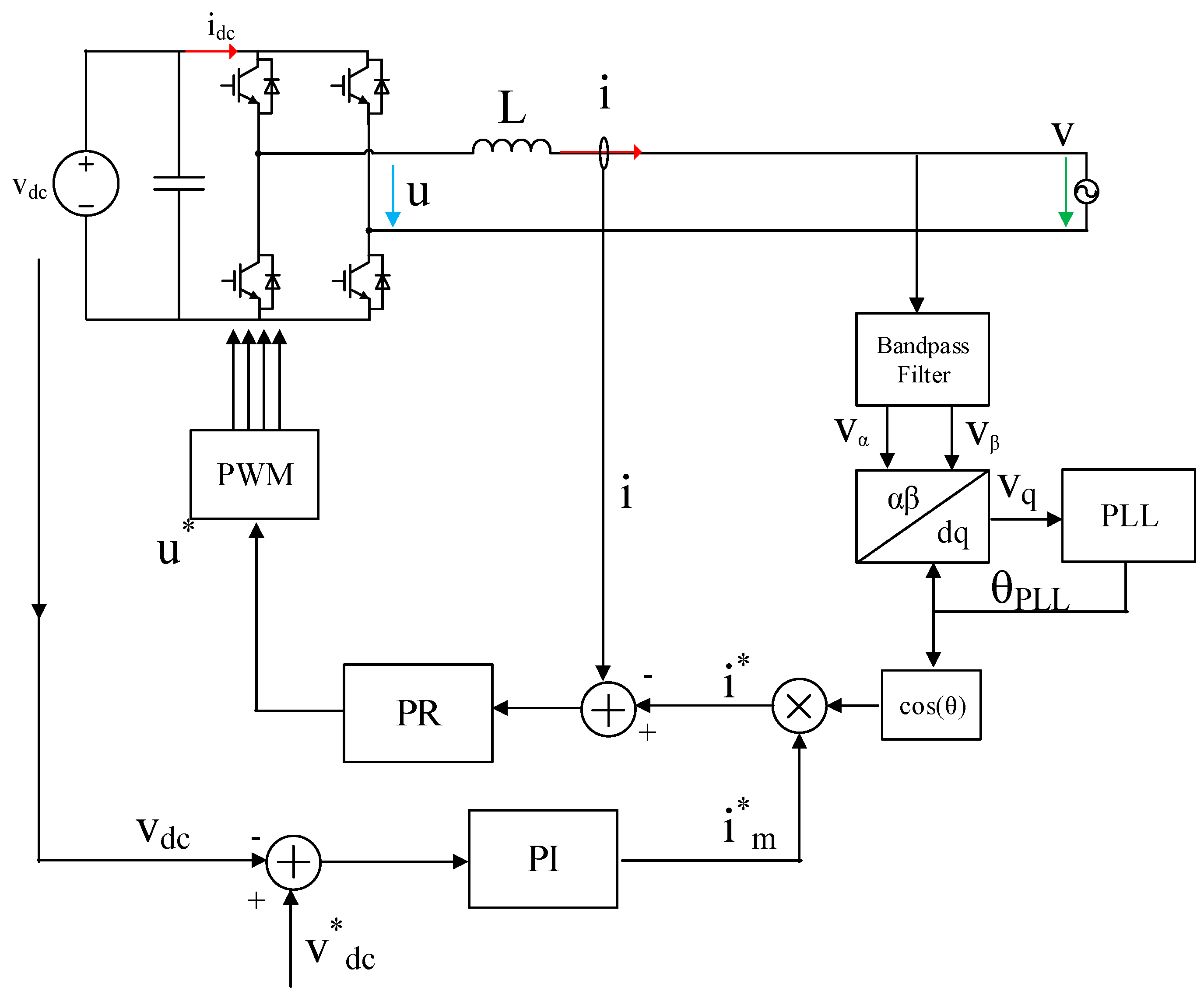
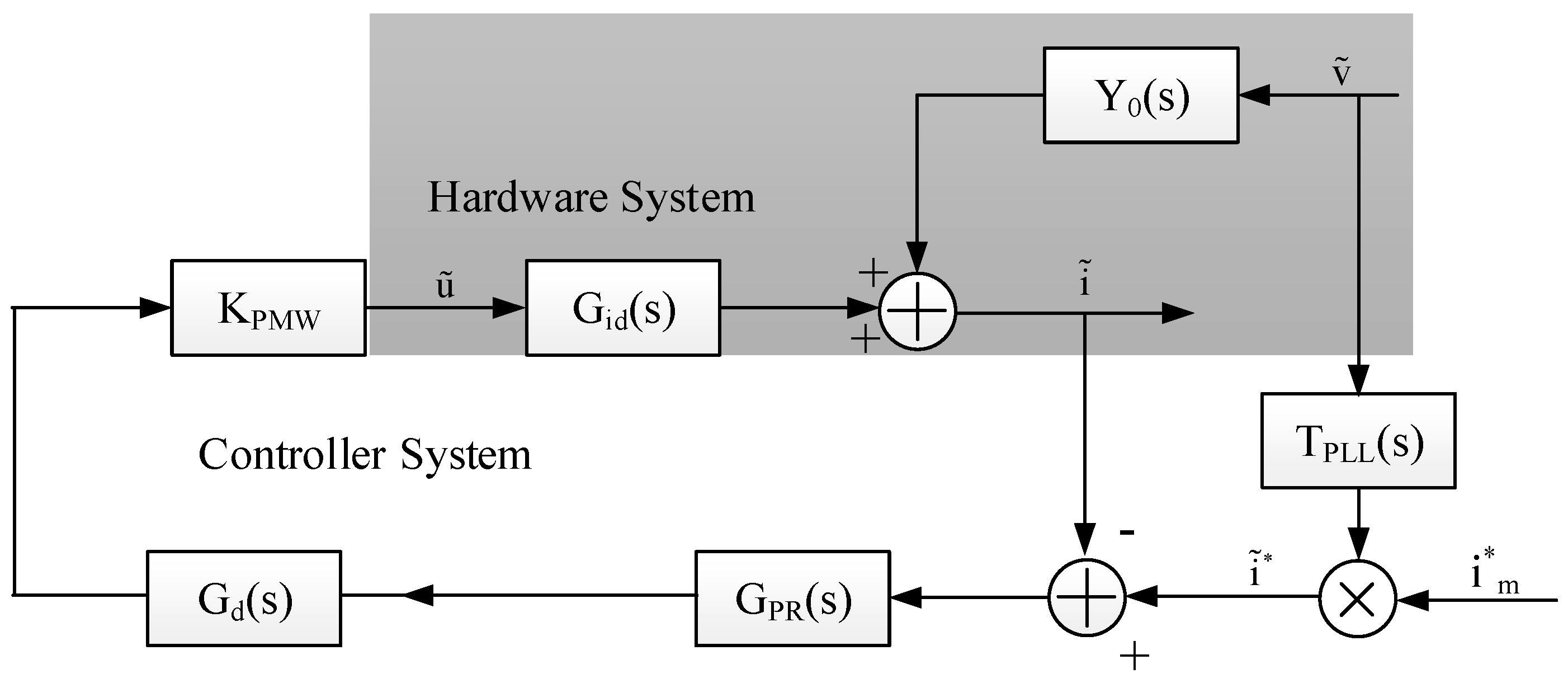
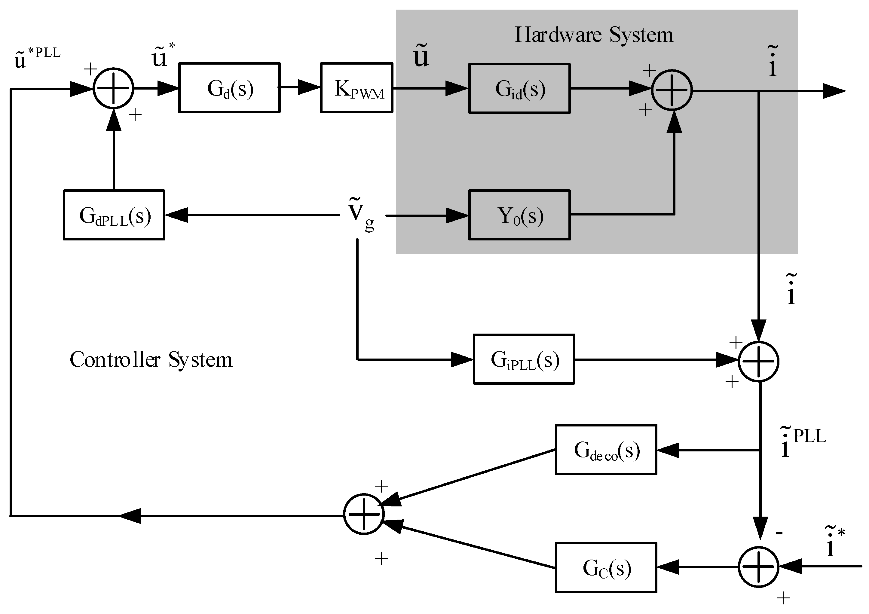
3. Modeling the Inverter in the Frequency-Domain

The research object of this article is a single-phase grid-connected inverter. Commonly used single-phase grid-connected inverter current control methods are

• proportional resonance (PR) based current control
• synchronous rotating frame (dq-transformation) based current control

3.1. PR-Based Current Control Method

The block diagram of a typical PR based current control single-phase inverter [23] is illustrated in Figure 5. The DC bus supplies power to the full bridge circuit with the voltage vdc. The output voltage of the full bridge circuit is u, i is the inverter output current. The full bridge circuit connects to the grid (v) through an inductive filter (L). The single-phase inverter obtains the phase angle of the grid voltage through a phase-locked loop in order to generate reference current i^* with the output from the DC voltage regulator i*m. The current loop controller is a quasi-PR regulator, which may robustly track the sinusoidal waveform without a static error, its transfer function is expressed in Equation (6).

$${\mathrm{G}}_{\mathrm{PR}}\left(\mathrm{s}\right)={\mathrm{K}}_{\mathrm{P}-\mathrm{PR}}+\frac{2{\mathrm{K}}_{\mathrm{P}-\mathrm{PR}}{\mathsf{\omega }}_c}{{\mathrm{s}}^2+2{\mathsf{\omega }}_c+{\mathsf{\omega }}_0^2}$$

(6)

where K_P-PR is the proportional coefficient; K_R-PR is the resonance coefficient; ω_c is the control bandwidth; ω₀ is the resonant frequency.

The output of the regulator is modulation the signal u*. The transfer function of the modulation signal u* to the output voltage of the full bridge circuit u is KPWM. The dynamics on the DC side are neglected here due to the large time constant on the DC side. The small signal model of the system is illustrated in Figure 6.

In Figure 6, the grey box groups the hardware system of the inverter, the rest represents the controller system. Y₀(s) is the output admittance of the inverter hardware, G_id(s) is the transfer function from the output voltage of the full bridge circuit u to output current i. T_PLL(s) is the transfer function from the grid side voltage v to the normalized current reference. The controller transfer function G_PR(s) is expressed in Equation (6), G_d(s) is the transfer function for the time delay in the digital control. The delay time consists of the calculation time in the controller and PWM modulation time. In this case, it is 1.5 times that of the sampling period [24,25].

The output admittance of the inverter hardware Y₀ can be derived by assuming the inverter output is zero; G_id can be derived by assuming the grid voltage is zero, as expressed in Equation (7).

$$\{\begin{array}{c}{\mathrm{Y}}_0\left(\mathrm{s}\right)=-\frac{1}{\mathrm{L}\mathrm{s}}\\ {\mathrm{G}}_{\mathrm{id}}\left(\mathrm{s}\right)=\frac{1}{\mathrm{L}\mathrm{s}}\end{array}$$

(7)

Without considering the effect of the PLL on the inverter, according to Figure 6, the transfer function from reference current i* to inverter output current i can be obtained, as expressed in Equation (8).

$$\mathrm{i}=\frac{{\mathrm{G}}_{\mathrm{PR}}\left(\mathrm{s}\right){\mathrm{G}}_{\mathrm{d}}\left(\mathrm{s}\right){\mathrm{K}}_{\mathrm{PWM}}}{{\mathrm{G}}_{\mathrm{PR}}\left(\mathrm{s}\right){\mathrm{G}}_{\mathrm{d}}\left(\mathrm{s}\right){\mathrm{K}}_{\mathrm{PWM}}+\mathrm{L}\mathrm{s}}{\mathrm{i}}^{\ast }-\frac{1}{{\mathrm{G}}_{\mathrm{PR}}\left(\mathrm{s}\right){\mathrm{G}}_{\mathrm{d}}\left(\mathrm{s}\right){\mathrm{K}}_{\mathrm{PWM}}+\mathrm{L}\mathrm{s}}\mathrm{v}$$

(8)

As shown in Figure 5 and Figure 6, the dynamics of the PLL will affect the performance of the inverter control, so the PLL also needs to be considered in the modeling of the inverter. The block diagram of a typical single-phase synchronous rotation frame (SRF) PLL is shown in Figure 7.

The operation principle of a single-phase SRF PLL is that by a bandpass-filter, two orthogonal grid voltages v_α and v_β will be obtained. Then the q-axis component of the grid voltage v_q can be calculated by performing a dq transformation on the grid voltage. Let vq become 0 through the closed loop control. When v_q = 0, the output of the regulator ω_PLL should be the angular velocity of the grid voltage ω_g, and its integral value θ_PLL should be the phase angle of the grid voltage θ_g.

In the steady state case, θ_PLL is equal to θ_g and the dq components of the voltage ${\mathrm{v}}_{\mathrm{dq}}^{\mathrm{PLL}}$ calculated by the PLL is equal to the dq components of the grid voltage vdq. In the case of non-steady state behavior (by small-signal perturbation), due to the influence of the control loop in PLL, the phase angle obtained by the PLL θ_PLL is no longer equal to the phase angle of the grid voltage θ_g, so the calculated dq component of the grid voltage ${\mathrm{v}}_{\mathrm{dq}}^{\mathrm{PLL}}$ in the controller system does not represent the exact grid situation. We then set the difference between θ_PLL and θg as δ_PLL. The transfer function from the grid voltage disturbance to the voltage disturbance in the controller is expressed in Equations (9) and (10).

$${\tilde{\mathrm{v}}}_{\mathrm{dq}}^{\mathrm{PLL}}={\mathrm{T}}_{{\mathsf{\delta }}_{\mathrm{PLL}}}{\tilde{\mathrm{v}}}_{\mathrm{dq}}$$

(9)

$${\mathrm{T}}_{{\mathsf{\delta }}_{\mathrm{PLL}}}=\left[\begin{array}{cc}\cos \left({\mathsf{\delta }}_{\mathrm{PLL}}\right)& \sin \left({\mathsf{\delta }}_{\mathrm{PLL}}\right)\\ -\sin \left({\mathsf{\delta }}_{\mathrm{PLL}}\right)& \cos \left({\mathsf{\delta }}_{\mathrm{PLL}}\right)\end{array}\right]$$

(10)

where the variable with the superscript PLL represents the dq component in the controller and the variable without the superscript represents the exact dq component.

Adding a small-signal perturbation to Equations (9) and (10) results in Equation (11).

$$\left[\begin{array}{c}{\mathrm{v}}_{\mathrm{d}}^{\mathrm{PLL}}+{\tilde{\mathrm{v}}}_{\mathrm{d}}^{\mathrm{PLL}}\\ {\mathrm{v}}_{\mathrm{q}}^{\mathrm{PLL}}+{\tilde{\mathrm{v}}}_{\mathrm{q}}^{\mathrm{PLL}}\end{array}\right]=\left[\begin{array}{cc}\cos \left({\tilde{\mathsf{\delta }}}_{\mathrm{PLL}}\right)& \sin \left({\tilde{\mathsf{\delta }}}_{\mathrm{PLL}}\right)\\ -\sin \left({\tilde{\mathsf{\delta }}}_{\mathrm{PLL}}\right)& \cos \left({\tilde{\mathsf{\delta }}}_{\mathrm{PLL}}\right)\end{array}\right]·\left[\begin{array}{c}{\mathrm{v}}_{\mathrm{d}}+{\tilde{\mathrm{v}}}_{\mathrm{d}}\\ {\mathrm{v}}_{\mathrm{q}}+{\tilde{\mathrm{v}}}_{\mathrm{q}}\end{array}\right]$$

(11)

When the phase angle perturbation is negligible, Equation (12) can be derived by Equation (11).

$$\left[\begin{array}{c}{\mathrm{v}}_{\mathrm{d}}^{\mathrm{PLL}}+{\tilde{\mathrm{v}}}_{\mathrm{d}}^{\mathrm{PLL}}\\ {\mathrm{v}}_{\mathrm{q}}^{\mathrm{PLL}}+{\tilde{\mathrm{v}}}_{\mathrm{q}}^{\mathrm{PLL}}\end{array}\right]\approx \left[\begin{array}{cc}1& {\tilde{\mathsf{\delta }}}_{\mathrm{PLL}}\\ -{\tilde{\mathsf{\delta }}}_{\mathrm{PLL}}& 1\end{array}\right]·\left[\begin{array}{c}{\mathrm{v}}_{\mathrm{d}}+{\tilde{\mathrm{v}}}_{\mathrm{d}}\\ {\mathrm{v}}_{\mathrm{q}}+{\tilde{\mathrm{v}}}_{\mathrm{q}}\end{array}\right]$$

(12)

By neglecting the steady state values in Equation (12), Equation (13) is obtained.

$$\left[\begin{array}{c}{\tilde{\mathrm{v}}}_{\mathrm{d}}^{\mathrm{PLL}}\\ {\tilde{\mathrm{v}}}_{\mathrm{q}}^{\mathrm{PLL}}\end{array}\right]\approx \left[\begin{array}{c}{\tilde{\mathsf{\delta }}}_{\mathrm{PLL}}{\mathrm{v}}_{\mathrm{q}}+{\tilde{\mathrm{v}}}_{\mathrm{d}}\\ -{\tilde{\mathsf{\delta }}}_{\mathrm{PLL}}{\mathrm{v}}_{\mathrm{d}}+{\tilde{\mathrm{v}}}_{\mathrm{q}}\end{array}\right]$$

(13)

According to Figure 7b, the output of the PLL can be derived as Equation (14).

$${\tilde{\mathsf{\delta }}}_{\mathrm{PLL}}={\tilde{\mathrm{v}}}_{\mathrm{q}}^{\mathrm{PLL}}{\mathrm{H}}_{\mathrm{PLL}}\left(\mathrm{s}\right)\frac{1}{\mathrm{s}}$$

(14)

By merging Equations (13) and (14), the transfer function of the PLL can be written as in Equation (15).

$$\frac{{\tilde{\mathsf{\delta }}}_{\mathrm{PLL}}}{{\tilde{\mathrm{v}}}_{\mathrm{q}}}={\mathrm{G}}_{\mathrm{PLL}}\left(\mathrm{s}\right)=\frac{{\mathrm{H}}_{\mathrm{PLL}}\left(\mathrm{s}\right)}{{\mathrm{H}}_{\mathrm{PLL}}\left(\mathrm{s}\right){\mathrm{v}}_{\mathrm{d}}+\mathrm{s}}$$

(15)

According to the block diagram (Figure 6) and considering the orthogonality of vα and vβ [26], the transfer function from the grid side voltage to the current reference can be derived, as expressed in Equation (16).

$$\frac{{\tilde{\mathrm{i}}}^{\ast }}{{\tilde{\mathrm{v}}}_{\mathsf{\alpha }}}=\frac{{\tilde{\mathrm{i}}}^{\ast }}{\tilde{\mathrm{v}}}={\mathrm{i}}_{\mathrm{m}}^{\ast }{\mathrm{T}}_{\mathrm{PLL}}(\mathrm{s})=\frac{{\mathrm{i}}_{\mathrm{m}}^{\ast }}{2}\frac{{\mathrm{H}}_{\mathrm{PLL}}\left(\mathrm{s}-\mathrm{j}{\mathsf{\omega }}_0\right)}{{\mathrm{H}}_{\mathrm{PLL}}\left(\mathrm{s}-\mathrm{j}{\mathsf{\omega }}_0\right){\mathrm{v}}_{\mathrm{d}}+(\mathrm{s}-\mathrm{j}{\mathsf{\omega }}_0)}$$

(16)

By applying Equation (16) into Equation (8), the relationship from the grid voltage to the inverter output current by considering the influence of PLL and the inverter output admittance will be obtained as shown in Equations (17) and (18), respectively.

$$\mathrm{i}=\frac{{\mathrm{i}}_{\mathrm{m}}^{\ast }{\mathrm{T}}_{\mathrm{PLL}}(\mathrm{s}){\mathrm{G}}_{\mathrm{PR}}\left(\mathrm{s}\right){\mathrm{G}}_{\mathrm{d}}\left(\mathrm{s}\right){\mathrm{K}}_{\mathrm{PWM}}-1}{{\mathrm{G}}_{\mathrm{PR}}\left(\mathrm{s}\right){\mathrm{G}}_{\mathrm{d}}\left(\mathrm{s}\right){\mathrm{K}}_{\mathrm{PWM}}+\mathrm{L}\mathrm{s}}\mathrm{v}$$

(17)

$${\mathrm{Y}}_{\mathrm{inv}}(\mathrm{s})=\frac{{\mathrm{i}}_{\mathrm{m}}^{\ast }{\mathrm{T}}_{\mathrm{PLL}}(\mathrm{s}){\mathrm{G}}_{\mathrm{PR}}\left(\mathrm{s}\right){\mathrm{G}}_{\mathrm{d}}\left(\mathrm{s}\right){\mathrm{K}}_{\mathrm{PWM}}-1}{{\mathrm{G}}_{\mathrm{PR}}\left(\mathrm{s}\right){\mathrm{G}}_{\mathrm{d}}\left(\mathrm{s}\right){\mathrm{K}}_{\mathrm{PWM}}+\mathrm{L}\mathrm{s}}$$

(18)

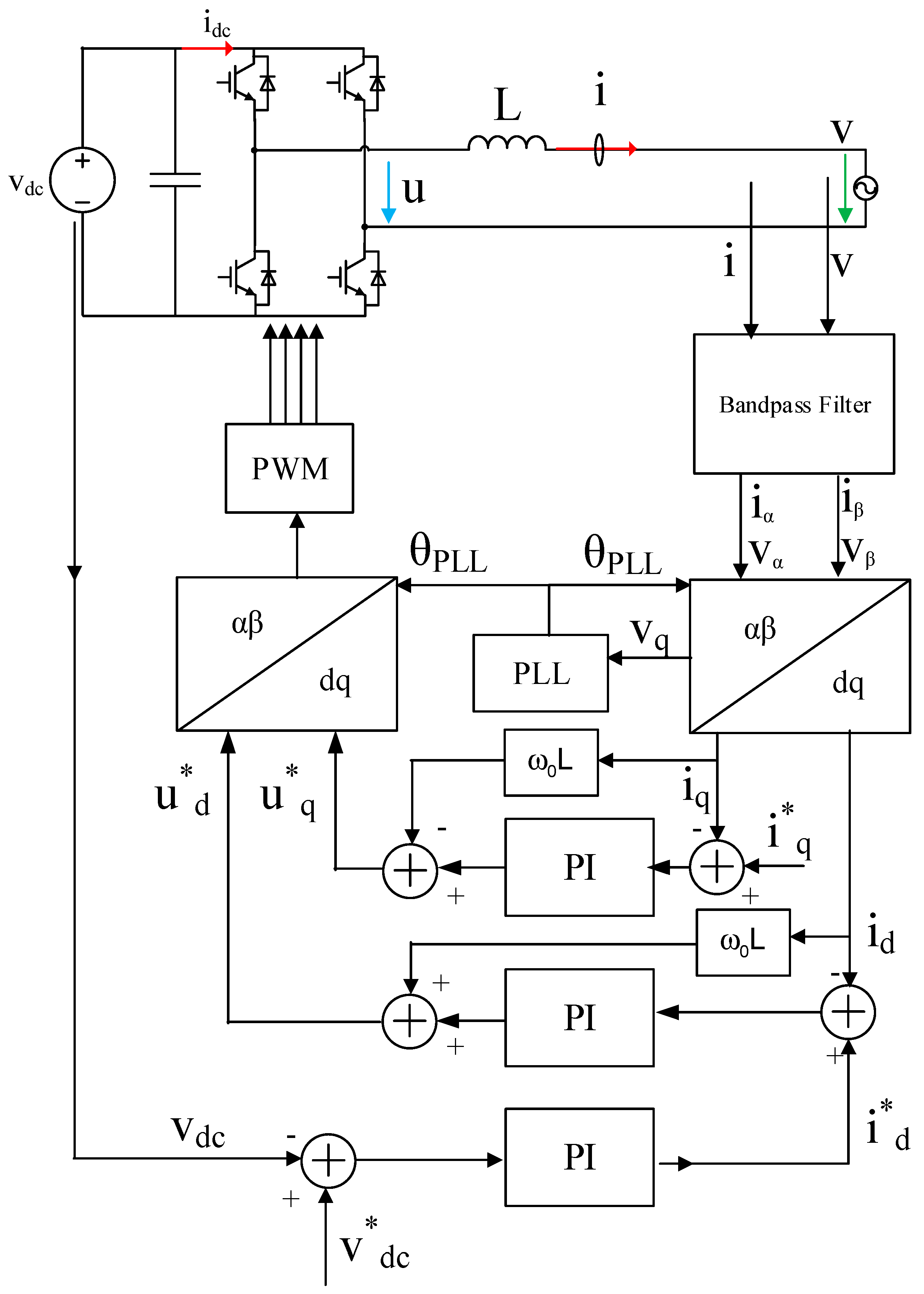
3.2. Synchronous Rotating Frame Based Current Control Method

The block diagram of a typical dq-transformation based current control single-phase inverter [23] is illustrated in Figure 8. Its hardware topology is the same as that of the PR-based current control inverter. The dq components of the inverter output current i_dq are obtained by dq transformation. Then the dq components of the current are controlled separately. The reference value of the dq components of the current i*_dq is obtained by a DC voltage regulator or/and calculated by the active/reactive power requirements. The output of the current regulator is converted into a reference of the inverter output voltage u*_dq after decoupling and inverse dq transformation.

As shown in Figure 8, the output phase angle of the PLL θ_PLL affects the results of the dq transformation and inverse dq transformation. With a small-signal perturbation, due to the PLL output difference δ_PLL, there is an influence on the value associated with the dq transformation. In order to present this influence, a small signal model is shown in Figure 9.

In Figure 9, the hardware system (in the grey box) is the same as in Figure 6. G_iPLL(s) is the transfer function matrix from the grid voltage disturbance to the inverter current disturbance in the controller, as expressed in Equation (19). G_uPLL(s) is the transfer function matrix from the grid voltage disturbance to the inverter output reference voltage disturbance in the controller, as expressed in Equation (20). G_deco(s) is the decoupling control matrix and G_C(s) is the current regulator matrix, as expressed in Equations (21) and (22), separately [27].

$${\tilde{\mathrm{i}}}_{\mathrm{dq}}^{\mathrm{PLL}}={\mathrm{G}}_{\mathrm{i}\mathrm{PLL}}(\mathrm{s}){\tilde{\mathrm{v}}}_{\mathrm{dq}}+{\tilde{\mathrm{i}}}_{\mathrm{dq}}$$

(19)

$${\tilde{\mathrm{u}}}_{\mathrm{dq}}^{\ast \mathrm{PLL}}={\mathrm{G}}_{\mathrm{uPLL}}{\tilde{\mathrm{v}}}_{\mathrm{dq}}+{\tilde{\mathrm{u}}}_{\mathrm{dq}}^{\ast }$$

(20)

$${\mathrm{G}}_{\mathrm{deco}}\left(\mathrm{s}\right)=\left[\begin{array}{cc}0& -\mathsf{\omega }\mathrm{L}\\ \mathsf{\omega }\mathrm{L}& 0\end{array}\right]$$

(21)

$${\mathrm{G}}_{\mathrm{C}}\left(\mathrm{s}\right)=\left[\begin{array}{cc}{\mathrm{K}}_{\mathrm{P}-\mathrm{C}}+\frac{{\mathrm{K}}_{\mathrm{I}-\mathrm{C}}}{\mathrm{s}}& 0\\ 0& {\mathrm{K}}_{\mathrm{P}-\mathrm{C}}+\frac{{\mathrm{K}}_{\mathrm{I}-\mathrm{C}}}{\mathrm{s}}\end{array}\right]$$

(22)

By applying the same derivation method in Section 3.1, Y₀ and G_id can be derived, as expressed in Equation (23).

$$\{\begin{array}{c}{\mathrm{Y}}_0\left(\mathrm{s}\right)=-\frac{1}{\mathrm{L}\left({\mathsf{\omega }}^2+{\mathrm{s}}^2\right)}\left[\begin{array}{cc}\mathrm{s}& \mathsf{\omega }\\ -\mathsf{\omega }& \mathrm{s}\end{array}\right]\\ {\mathrm{G}}_{\mathrm{i}\mathrm{d}}\left(\mathrm{s}\right)=\frac{1}{\mathrm{L}\left({\mathsf{\omega }}^2+{\mathrm{s}}^2\right)}\left[\begin{array}{cc}\mathrm{s}& \mathsf{\omega }\\ -\mathsf{\omega }& \mathrm{s}\end{array}\right]\end{array}$$

(23)

Small-signal perturbation is added to Equations (19), (20), and (10) to derive Equations (24) and (25).

$$\left[\begin{array}{c}{\mathrm{I}}_{\mathrm{d}}^{\mathrm{PLL}}+{\tilde{\mathrm{i}}}_{\mathrm{d}}^{\mathrm{PLL}}\\ {\mathrm{I}}_{\mathrm{q}}^{\mathrm{PLL}}+{\tilde{\mathrm{i}}}_{\mathrm{q}}^{\mathrm{PLL}}\end{array}\right]\approx \left[\begin{array}{cc}1& {\tilde{\mathsf{\delta }}}_{\mathrm{PLL}}\\ -{\tilde{\mathsf{\delta }}}_{\mathrm{PLL}}& 1\end{array}\right]·\left[\begin{array}{c}{\mathrm{I}}_{\mathrm{d}}+{\tilde{\mathrm{i}}}_{\mathrm{d}}\\ {\mathrm{I}}_{\mathrm{q}}+{\tilde{\mathrm{i}}}_{\mathrm{q}}\end{array}\right]$$

(24)

$$\left[\begin{array}{c}{\mathrm{U}}_{\mathrm{d}}^{\ast \mathrm{PLL}}+{\tilde{\mathrm{u}}}_{\mathrm{d}}^{\ast \mathrm{PLL}}\\ {\mathrm{U}}_{\mathrm{q}}^{\ast \mathrm{PLL}}+{\tilde{\mathrm{u}}}_{\mathrm{q}}^{\ast \mathrm{PLL}}\end{array}\right]\approx \left[\begin{array}{cc}1& {\tilde{\mathsf{\delta }}}_{\mathrm{PLL}}\\ -{\tilde{\mathsf{\delta }}}_{\mathrm{PLL}}& 1\end{array}\right]·\left[\begin{array}{c}{\mathrm{U}}_{\mathrm{d}}^{\ast }+{\tilde{\mathrm{u}}}_{\mathrm{d}}^{\ast }\\ {\mathrm{U}}_{\mathrm{q}}^{\ast }+{\tilde{\mathrm{u}}}_{\mathrm{q}}^{\ast }\end{array}\right]$$

(25)

By eliminating the steady state values in Equations (24) and (25), we obtain Equations (26) and (27).

$$\left[\begin{array}{c}{\tilde{\mathrm{i}}}_{\mathrm{d}}^{\mathrm{PLL}}\\ {\tilde{\mathrm{i}}}_{\mathrm{q}}^{\mathrm{PLL}}\end{array}\right]\approx \left[\begin{array}{c}{\tilde{\mathrm{i}}}_{\mathrm{d}}+{\tilde{\mathsf{\delta }}}_{\mathrm{PLL}}{\mathrm{I}}_{\mathrm{q}}\\ {\tilde{\mathrm{i}}}_{\mathrm{q}}-{\tilde{\mathsf{\delta }}}_{\mathrm{PLL}}{\mathrm{I}}_{\mathrm{d}}\end{array}\right]$$

(26)

$$\left[\begin{array}{c}{\tilde{\mathrm{u}}}_{\mathrm{d}}^{\ast \mathrm{PLL}}\\ {\tilde{\mathrm{u}}}_{\mathrm{q}}^{\ast \mathrm{PLL}}\end{array}\right]\approx \left[\begin{array}{c}{\tilde{\mathrm{u}}}_{\mathrm{d}}^{\ast }+{\tilde{\mathsf{\delta }}}_{\mathrm{PLL}}{\mathrm{U}}_{\mathrm{q}}^{\ast }\\ {\tilde{\mathrm{u}}}_{\mathrm{q}}^{\ast }-{\tilde{\mathsf{\delta }}}_{\mathrm{PLL}}{\mathrm{U}}_{\mathrm{d}}^{\ast }\end{array}\right]$$

(27)

By putting Equation (15) into Equations (26) and (27), Equations (28) and (29) are obtained.

$$\left[\begin{array}{c}{\tilde{\mathrm{i}}}_{\mathrm{d}}^{\mathrm{PLL}}\\ {\tilde{\mathrm{i}}}_{\mathrm{q}}^{\mathrm{PLL}}\end{array}\right]\approx \left[\begin{array}{cc}0& {\mathrm{G}}_{\mathrm{PLL}}{\mathrm{I}}_{\mathrm{q}}\\ 0& -{\mathrm{G}}_{\mathrm{PLL}}{\mathrm{I}}_{\mathrm{d}}\end{array}\right]·\left[\begin{array}{c}{\tilde{\mathrm{v}}}_{\mathrm{d}}\\ {\tilde{\mathrm{v}}}_{\mathrm{q}}\end{array}\right]+\left[\begin{array}{c}{\tilde{\mathrm{i}}}_{\mathrm{d}}\\ {\tilde{\mathrm{i}}}_{\mathrm{q}}\end{array}\right]$$

(28)

$$\left[\begin{array}{c}{\tilde{\mathrm{u}}}_{\mathrm{d}}^{\ast }\\ {\tilde{\mathrm{u}}}_{\mathrm{q}}^{\ast }\end{array}\right]\approx \left[\begin{array}{cc}0& -{\mathrm{G}}_{\mathrm{PLL}}{\mathrm{U}}_{\mathrm{q}}^{\ast }\\ 0& {\mathrm{G}}_{\mathrm{PLL}}{\mathrm{U}}_{\mathrm{d}}^{\ast }\end{array}\right]·\left[\begin{array}{c}{\tilde{\mathrm{v}}}_{\mathrm{d}}\\ {\tilde{\mathrm{v}}}_{\mathrm{q}}\end{array}\right]+\left[\begin{array}{c}{\tilde{\mathrm{u}}}_{\mathrm{d}}^{\ast \mathrm{PLL}}\\ {\tilde{\mathrm{u}}}_{\mathrm{q}}^{\ast \mathrm{PLL}}\end{array}\right]$$

(29)

According to Figure 9 (the relationship from the grid voltage to the inverter output current) by considering the influence of PLL, the inverter output admittance Y_inv and the current loop control transfer function H_C can be derived, as shown in Equations (30)–(32), respectively.

$$\mathrm{i}={\mathrm{H}}_{\mathrm{C}}\left(\mathrm{s}\right){\mathrm{i}}^{\ast }+{\mathrm{Y}}_{\mathrm{inv}}\left(\mathrm{s}\right)\mathrm{v}$$

(30)

$${\mathrm{Y}}_{\mathrm{inv}}=\frac{{\mathrm{Y}}_0\left({\mathrm{G}}_{\mathrm{d}}{\mathrm{K}}_{\mathrm{PWM}}\left({\mathrm{G}}_{\mathrm{i}\mathrm{PLL}}\left({\mathrm{G}}_{\mathrm{deco}}-{\mathrm{G}}_{\mathrm{c}}\right)+{\mathrm{G}}_{\mathrm{d}\mathrm{PLL}}\right)-\mathrm{I}\right)}{\mathrm{I}+{\mathrm{G}}_{\mathrm{d}}{\mathrm{Y}}_0{\mathrm{K}}_{\mathrm{PWM}}\left({\mathrm{G}}_{\mathrm{deco}}-{\mathrm{G}}_{\mathrm{c}}\right)}$$

(31)

$${\mathrm{H}}_{\mathrm{C}}=\frac{{\mathrm{Y}}_0{\mathrm{G}}_{\mathrm{C}}{\mathrm{G}}_{\mathrm{d}}{\mathrm{K}}_{\mathrm{PWM}}}{\mathrm{I}+{\mathrm{Y}}_0{\mathrm{G}}_{\mathrm{d}}{\mathrm{K}}_{\mathrm{PWM}}\left({\mathrm{G}}_{\mathrm{deco}}-{\mathrm{G}}_{\mathrm{C}}\right)}$$

(32)

I represents the identity matrix.

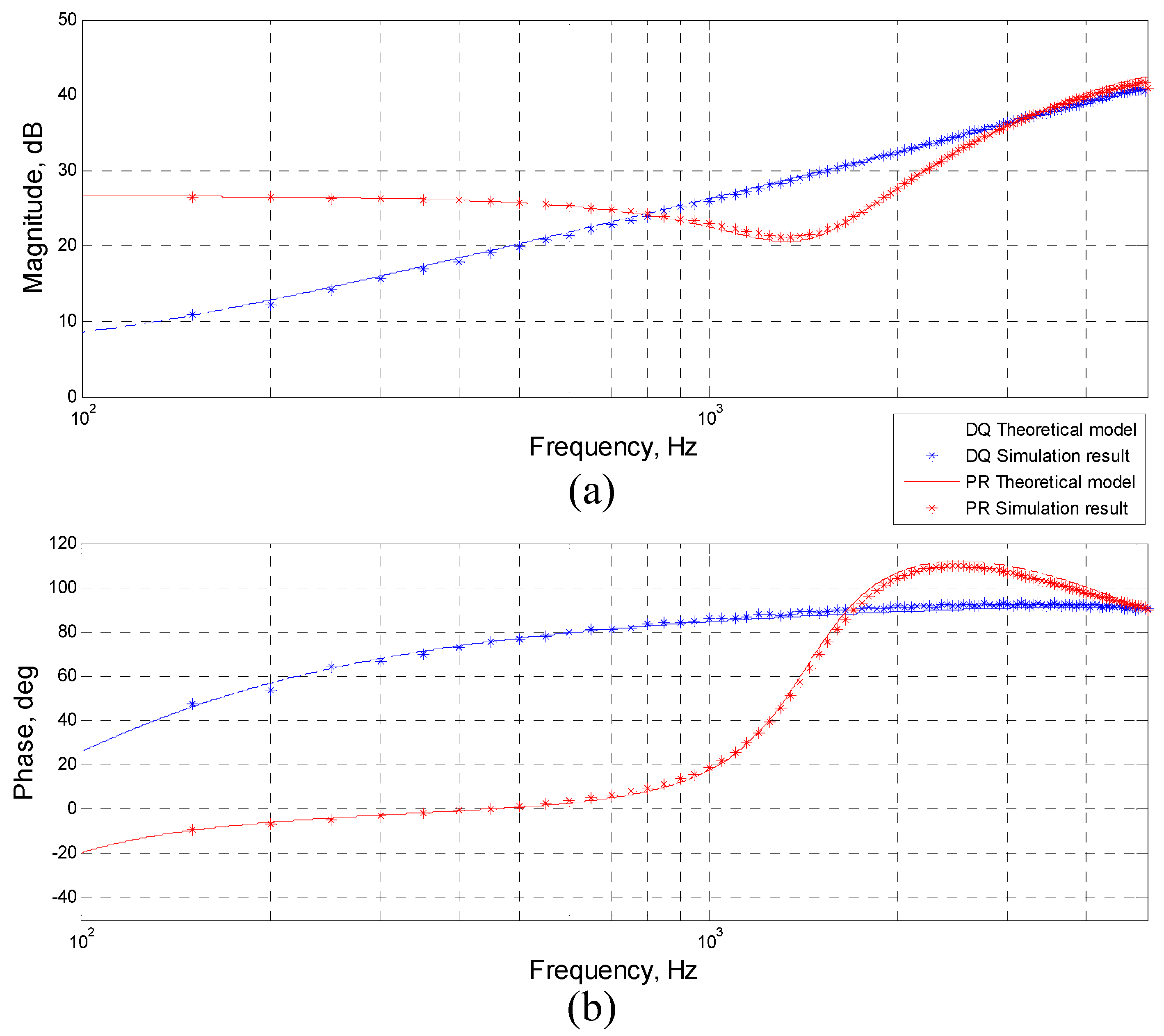
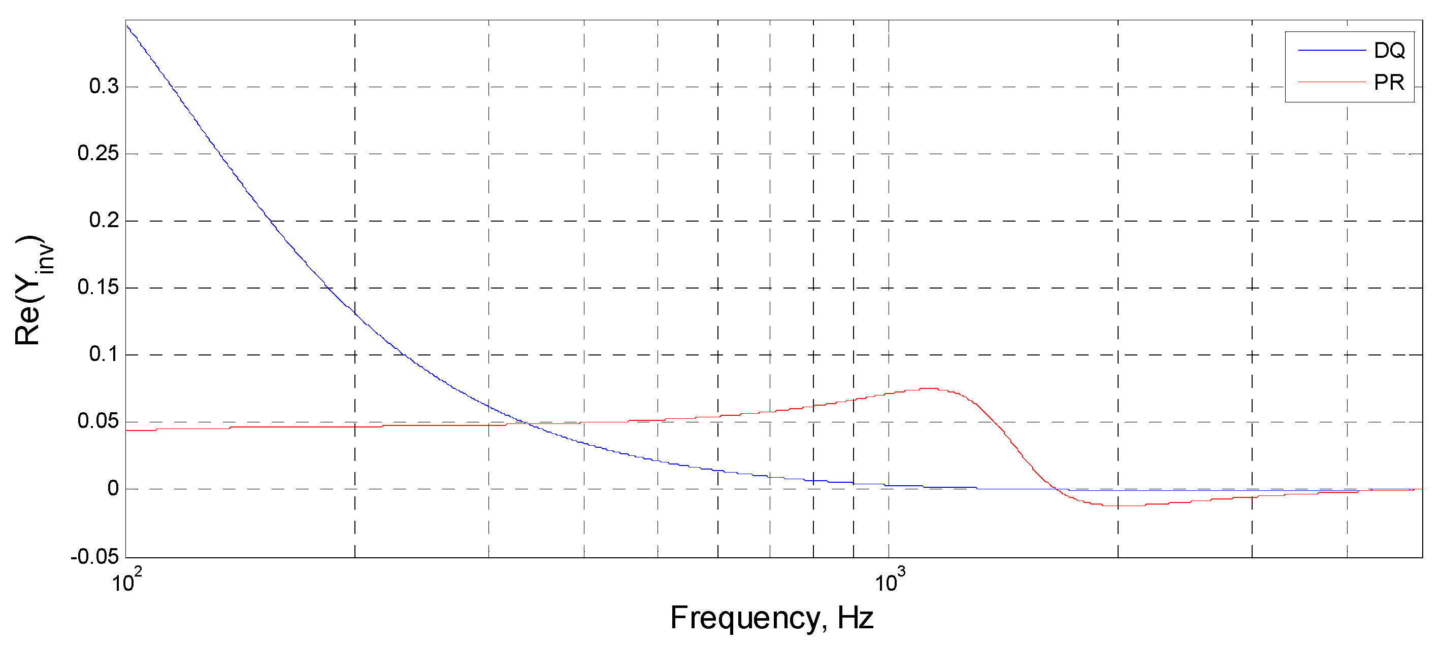
4. Simulation Verification

The system as described above is analyzed analytically in the time domain (EMT-simulation) as well as in the frequency domain, using the equations from Section 3. The parameters in

Table 1. The parameters of the inverters.

Parameter	DQ	PR
Rated power	3.3 kW
Rated voltage	230 V
Filter inductor	3.5 mH
PLL bandwidth	25 Hz
Sampling frequency	10 kHz
KP-C	2.46	/
KI-C	548.81	/
KP-PR	/	34.99
KR-PR	/	400
ωc	/	π

are applied during the output admittance calculation and simulation. In this article, the influence of the d-axis component on the d-axis component of the inverter is analyzed. The analysis methods of other influences are similar to this and will not be repeated. Parameters were selected to achieve the same behavior as measured.

Verification

We put the parameters in Table 1 into Equations (18) and (31) to illustrate the bode diagram of the inverter output impedance. In the simulation, a small harmonic voltage of 100–5000 Hz is added to the grid voltage, the inverter output current is measured, and the output impedance of the inverter is obtained after the calculation of the measured data, as shown in Figure 10.

As shown in Figure 10, the analytic calculation results (Equations (18) and (31)) and the results from the simulation match very well. The accuracy of the linearized analytical model in the frequency domain has been verified.

The real part of the inverter output admittance Re{Y(jω)} is illustrated in Figure 11.

As shown in Figure 11, both the dq-based control method (blue line) and PR-based control method (red line) enter the range with the negative real part of the output admittance near about 1700 Hz. This means that both control methods will be not stable if the resonance point of the grid is above 1700 Hz (Critical resonant frequency).

Verification will be performed in the simulation. In the simulation, the grid impedance consists of a CL circuit. The filter inductance of the inverter L, the grid capacitance Cg and the grid inductance Lg together form an LCL resonant circuit. Lg is given as 49.5 μH, corresponding to a 400 m cable length. The total grid capacitance, taking into account all the LV-cables in the analyzed system, will be estimated so that a specified resonance frequency is achieved (Equation (33)).

$${\mathrm{C}}_{\mathrm{g}}=\frac{\mathrm{L}+{\mathrm{L}}_{\mathrm{g}}}{4\mathrm{L}{\mathrm{L}}_{\mathrm{g}}{\left(\pi {\mathrm{f}}_{\mathrm{r}}\right)}^2}$$

(33)

The resonant frequencies are set to 1530 Hz and 1730 Hz, respectively. To demonstrate the instability effect, the time domain simulation is started without capacitance and after 0.3 s, the capacitance is connected, forming an LCL circuit. The simulation results are shown in Figure 12.

As shown in Figure 12a,c, the inverter-grid system with the dq-based control method oscillates slightly after 0.3 s since the Re{Y_inv(jω)} of the inverter with the dq-based control method is near 0 in a large frequency range (1000 Hz~5000 Hz), as shown in Figure 11.

As shown in Figure 12b, when f_r = 1530 Hz is less than the critical resonant frequency (1700 Hz), the inverter-grid system with the PR-based control method is stable after 0.3 s. As shown in Figure 12f, when f_r = 1730 is larger than the critical resonant frequency (1700 Hz), the system is unstable after 0.3 s.

By comparing Figure 12c,d with the same system resonant frequency, the dq-based control method is critically stable and the PR-based control method is resonance instable. Since the dq-based control method (Figure 11a, blue line) is always above the PR-based control method (Figure 11a, red line) after entering the range with the negative real part of the output admittance, this means that the dq-based control method has a larger stability margin than the PR-based control method.

5. Analysis of the Influence of the Control Parameter and Improvement Methods

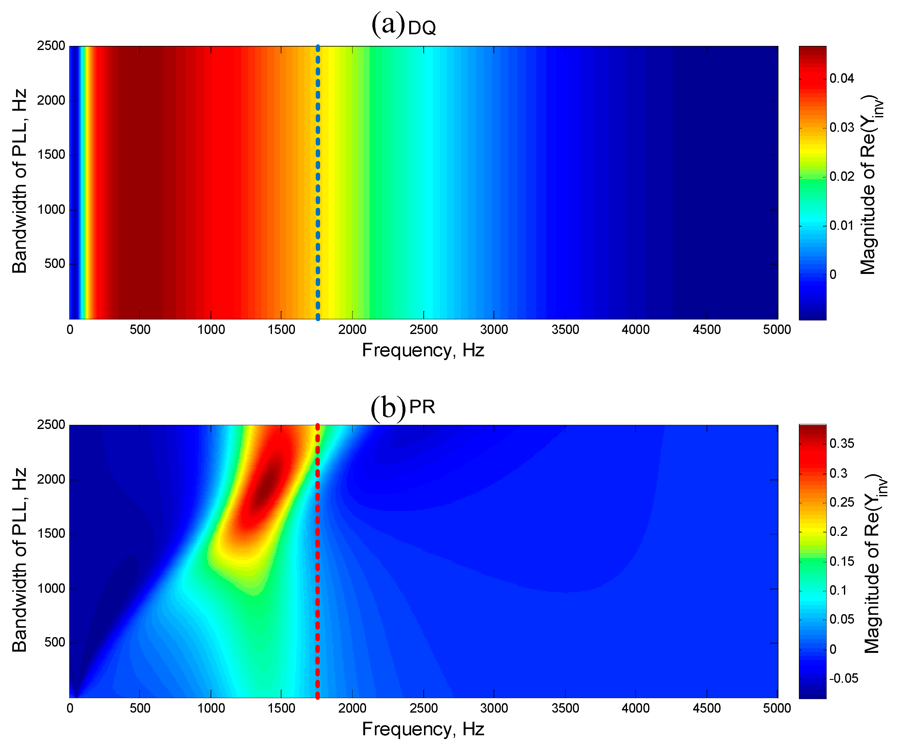
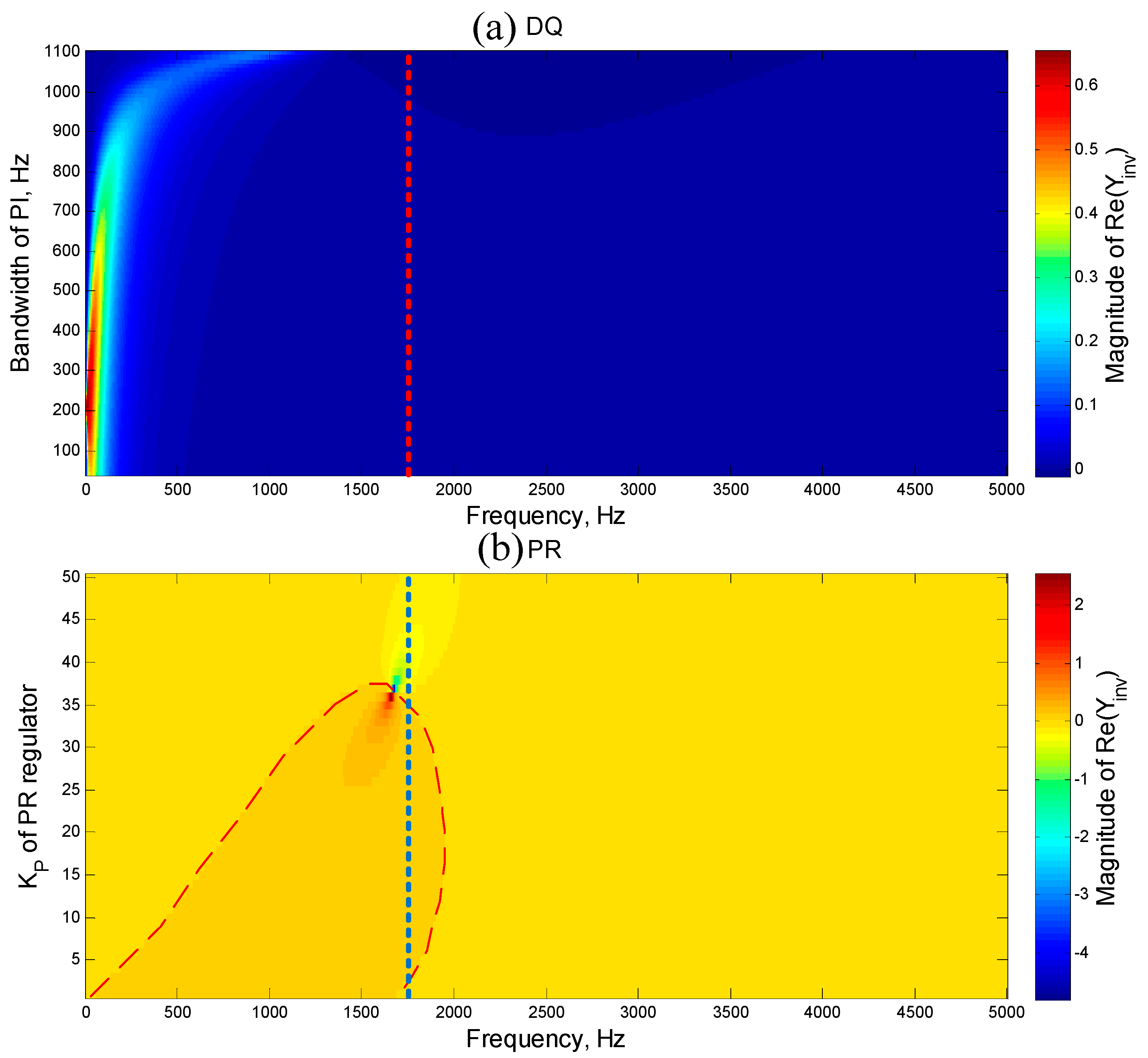
5.1. Analysis of the Influence of the Control Parameter

Figure 13 illustrates the influence of the PLL bandwidth on Re{Yinv(jω)}, the abscissa shows the frequency, the ordinate shows the PLL bandwidth and different colors represent Re{Yinv(jω)}. The parameters in Table 1 are used to generate Figure 13.

In Figure 13, the abscissa represents the frequency of Re{Y_inv(jω)}, the ordinate represents the PLL bandwidth and the color in the figure represents the amplitude of the Re{Y_inv(jω)}, with warm colors representing larger amplitudes and cool colors representing smaller amplitudes. Dark blue represents the negative amplitude of the Re{Y_inv(jω)}. The blue vertical dotted line in Figure 13a and red vertical dotted line in Figure 13b represent the 1700 Hz line.

As shown in Figure 13a, the increase of the PLL bandwidth has no effect on the Re{Y_inv(jω)} of the dq-based control method. With the increasing PLL bandwidth, the negative area of the Re{Y_inv(jω)} of the PR-based control method expands at a low frequency (Figure 13b). The positive area shrinks even though the amplitude increases. In general, the stability frequency area of the system becomes smaller.

In order to specifically analyze the influence of the control parameters on a certain frequency, 1700 Hz is selected as the target frequency for analysis in this article. The increased PLL bandwidth (>2000 Hz) will cause the Re{Y_inv(jω)} of the PR-based control method to enter a stable area at 1730 Hz (Figure 13b). Thus, when the resonant frequency of the grid impedance is around 1700 Hz, the inverter-grid system can still be stable.

In Figure 14, the abscissa represents the frequency of Re{Y_inv(jω)}, the ordinate represents the PI bandwidth for the current control loop of the dq-based control method (Figure 14a), and the proportion coefficient KP-PR of the PR-based control method (Figure 14b). The red vertical dotted line in Figure 14a and the blue vertical dotted line in Figure 14b represents the 1700 Hz line.

By increasing the PI bandwidth for the current control loop of the dq-based control method, the negative area of the Re{Y_inv(jω)} expands at a low frequency, the positive area moves to a higher frequency area, and the amplitude peak of Re{Y_inv(jω)} also decreases, as shown in Figure 14a. For the PR-based control method, by increasing the proportion coefficient K_P−PR, the positive area (Figure 14b, in the red dotted box) shrinks. Thus, increasing the PI control bandwidth or proportion coefficient will result in a reduction in the system’s stable frequency area.

By increasing the PI bandwidth for the current control loop of the dq-based control method, the negative area of the Re{Y_inv(jω)} expands at a low frequency, the positive area moves to a higher frequency area, and the amplitude peak of Re{Y_inv(jω)} also decreases, as shown in Figure 14a. For the PR-based control method, by increasing the proportion coefficient K_P-PR, the positive area (Figure 14b, in the red dotted box) shrinks. Thus, increasing the PI control bandwidth or the proportion coefficient will result in a reduction in the system’s stable frequency area.

When the frequency is 1700 Hz, the increase of the PI bandwidth for the current control loop of the dq-based control method cannot significantly change the amplitude of the Re{Y_inv(jω)}, as shown in Figure 14a (the red line). The increase of the proportion coefficient K_P−PR for the current control loop of the PR-based control method will let Re{Y_inv(jω)} < 0 if K_P−PR > 34. In other words, when K_P−PR < 34, if the resonant frequency of the grid impedance is near 1700 Hz, the inverter will be stable.

In addition to reducing the PLL bandwidth and current loop control bandwidth, increasing the filter inductance of the inverter or reducing the delay of the controller can also extend the positive range of Re{Y_inv(jω)}. However, these parameters are limited by the inverter’s hardware and controller performance, it is not convenient for them to be changed in practical operations.

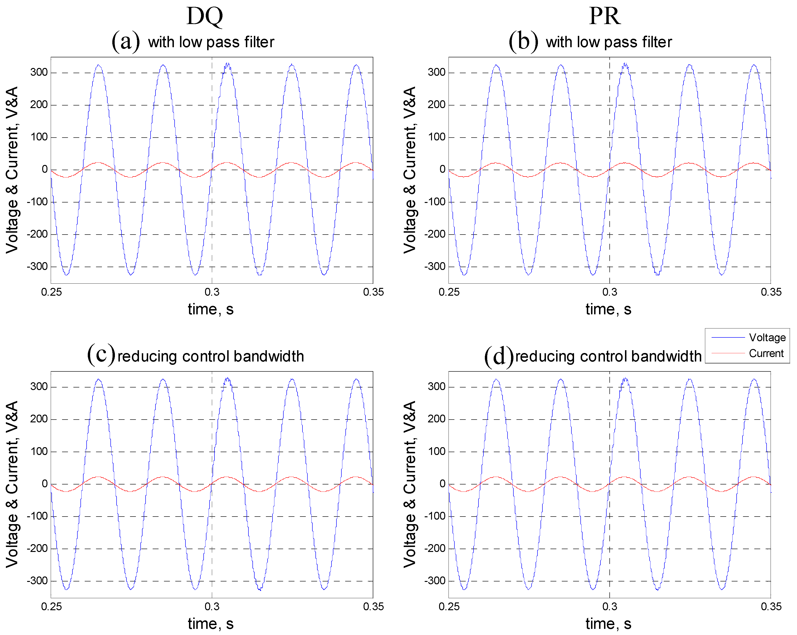
5.2. Improvement Methods

As discussed in Section 5.1, choosing a lower PLL bandwidth and current control bandwidth let Re{Y_inv(jω)} expand its positive area to increase the stability margin of the inverter. In the case that the resonant frequency of the grid impedance is unknown, the method of reducing the control bandwidth can maximize the robustness of the inverter.

Another way to improve the stability is to install the filter on the output side of the inverter to eliminate the influence of the grid impedance resonance on the inverter. If the resonant frequency of the grid impedance is known, a low-pass filter with a cutoff frequency below the resonant frequency or a notch filter can be connected on the output side of the inverter.

To demonstrate the effect of these two improved methods, a time domain simulation with the same process and parameters of Figure 12 is carried out. The resonant frequency of the grid impedance is set to 1730 Hz, the same as in Figure 12c,d. The time domain simulation is started without the capacitance and after 0.3 s, the capacitance is connected, forming an LCL circuit. The simulation results are shown in Figure 15.

Since the resonant frequency of the grid impedance is 1730 Hz, a low-pass filter with a cutoff frequency of 850 Hz is connected to the output side of the inverter in the simulation. As shown in Figure 15a,b, the inverter-grid system is stable after 0.3 s. Comparing Figure 13c,d and Figure 15a,b, the stability of the inverter-grid system with two different control methods can be seen to have significantly improved.

The simulation results for reducing the control bandwidth are shown in Figure 15c,d. The PLL bandwidth and current control bandwidth are simultaneously reduced to 20% of the original value (Table 1). As shown in Figure 13c,d, the inverter-grid system is stable after 0.3 s. Comparing Figure 12c,d and Figure 15c,d, the stability of the inverter-grid system with the two different control methods have been significantly improved.

6. Conclusions

In this article, the resonance instability phenomenon that was found during tests of a photovoltaic charging station is analyzed. The interaction of a resonance situation in the grid impedance and non-passivity of the inverter in that frequency range causes the system formed by the inverter and grid to be non-stable.

The inverter output admittance determines whether the inverter is passive or not. In order to analyze the inverter output admittance, the single-phase inverter system is modelled, taking into account the two common control methods. These are, respectively, the PR-based current control and the synchronous rotating frame based current control methods (dq-based). In order to consider the effect of the PLL on the output admittance, a linear small signal model is used for the PLL modeling.

This article verified the modeling by simulation. The analytical model shows that the real part of the inverter output admittance is negative for frequencies above 1700 Hz. In case the resonant frequency of the grid impedance exceeds 1700 Hz, the inverter-grid system will be unstable. The results are confirmed by the time domain simulation.

This article further analyzes the influence of different control parameters on the inverter output admittance. The analysis shows that the PLL bandwidth and the control parameters of the current loop will have an influence on the output admittance of the inverter. By adjusting these parameters, the inverter-grid system may be prevented from being unstable at certain resonant frequencies.

On the basis of the above analysis, this article gives two methods to improve stability: connecting a low pass filter or reducing the control bandwidth. The simulation results show that both of these methods can significantly improve the stability of the inverter-power grid system.

References

1. Biresselioglu, M.E.; Demirbag Kaplan, M.; Yilmaz, B.K. Electric mobility in Europe: A comprehensive review of motivators and barriers in decision making processes. Transp. Res. Part A Policy Pract. 2018, 109, 1–13. [Google Scholar] [CrossRef]
2. Fathabadi, H. Novel grid-connected solar/wind powered electric vehicle charging station with vehicle-to-grid technology. Energy 2017, 132, 1–11. [Google Scholar] [CrossRef]
3. Nunes, P.; Figueiredo, R.; Brito, M.C. The use of parking lots to solar-charge electric vehicles. Renew. Sustain. Energy Rev. 2016, 66, 679–693. [Google Scholar] [CrossRef]
4. Redpath, D.A.G.; McIlveen-Wright, D.; Kattakayam, T.; Hewitt, N.J.; Karlowski, J.; Bardi, U. Battery powered electric vehicles charged via solar photovoltaic arrays developed for light agricultural duties in remote hilly areas in the Southern Mediterranean region. J. Clean. Prod. 2011, 19, 2034–2048. [Google Scholar] [CrossRef]
5. Ji, S.; Cherry, C.R.; Han, L.D.; Jordan, D.A. Electric bike sharing: Simulation of user demand and system availability. J. Clean. Prod. 2014, 85, 250–257. [Google Scholar] [CrossRef]
6. Apostolou, G.; Reinders, A.; Geurs, K. An Overview of Existing Experiences with Solar-Powered E-Bikes. Energies 2018, 11, 2129. [Google Scholar] [CrossRef]
7. Apostolou, G.; Guers, K.; Reinders, A. Technical performance and user aspects of solar powered e-bikes—Results of a field study in The Netherlands. Presented at the DIT–ESEIA Conference on Smart Energy Systems in Cities and Regions, Dublin, Ireland, 10–12 April 2018. [Google Scholar]
8. Zhao, M.; Yuan, X.; Hu, J.; Yan, Y. Voltage Dynamics of Current Control Time-Scale in a VSC-Connected Weak Grid. IEEE Trans. Power Syst. 2016, 31, 2925–2937. [Google Scholar] [CrossRef]
9. Krein, P.T.; Bentsman, J.; Bass, R.M.; Lesieutre, B.L. On the use of averaging for the analysis of power electronic systems. IEEE Trans. Power Electron. 1990, 5, 182–190. [Google Scholar] [CrossRef]
10. Sun, J. AC power electronic systems: Stability and power quality. In Proceedings of the 2008 11th Workshop on Control and Modeling for Power Electronics, Zurich, Switzerland, 17–20 August 2008; pp. 1–10. [Google Scholar]
11. Kroutikova, N.; Hernandez-Aramburo, C.A.; Green, T.C. State-space model of grid-connected inverters under current control mode. IET Electr. Power Appl. 2007, 1, 329. [Google Scholar] [CrossRef] [Green Version]
12. Bengtsson, T.; Bickel, P.; Li, B. Curse-of-dimensionality revisited: Collapse of the particle filter in very large scale systems. In Institute of Mathematical Statistics Collections; Institute of Mathematical Statistics: Beachwood, OH, USA, 2008; pp. 316–334. ISBN 978-0-940600-74-4. [Google Scholar]
13. Sun, J. Impedance-Based Stability Criterion for Grid-Connected Inverters. IEEE Trans. Power Electron. 2011, 26, 3075–3078. [Google Scholar] [CrossRef]
14. Willems, J.C. Dissipative Dynamical Systems. Eur. J. Control 2007, 13, 134–151. [Google Scholar] [CrossRef]
15. Hu, H.; Tao, H.; Blaabjerg, F.; Wang, X.; He, Z.; Gao, S. Train–Network Interactions and Stability Evaluation in High-Speed Railways–Part I: Phenomena and Modeling. IEEE Trans. Power Electron. 2018, 33, 4627–4642. [Google Scholar] [CrossRef]
16. Pan, P.; Hu, H.; Yang, X.; Blaabjerg, F.; Wang, X.; He, Z. Impedance Measurement of Traction Network and Electric Train for Stability Analysis in High-Speed Railways. IEEE Trans. Power Electron. 2018, 33, 10086–10100. [Google Scholar] [CrossRef]
17. Reinders, A.; de Respinis, M.; van Loon, J.; Stekelenburg, A.; Bliek, F.; Schram, W.; van Sark, W.; Esteri, T.; Uebermasser, S.; Lehfuss, F.; et al. Co-evolution of smart energy products and services: A novel approach towards smart grids. In Proceedings of the 2016 Asian Conference on Energy, Power and Transportation Electrification, Singapore, 25–27 October 2016; pp. 1–6. [Google Scholar]
18. Canadian Solar. All-Black CS6K-270-275-280 M. Available online: https://www.canadiansolar.com/downloads/datasheets/v5.531/canadian_solar-datasheet-allblack-CS6K-M-v5.531en.pdf (accessed on 30 November 2018).
19. olax Power. X1 Series User Manual. Available online: https://www.solaxpower.com/wp-content/uploads/2017/01/X1-Mini-Install-Manual.pdf (accessed on 30 November 2018).
20. Ciobotaru, M.; Agelidis, V.; Teodorescu, R. Line impedance estimation using model based identification technique. In Proceedings of the 2011 14th European Conference on Power Electronics and Applications, Birmingham, UK, 30 August–1 September 2011; pp. 1–9. [Google Scholar]
21. Guo, X.; Wu, W.; Chen, Z. Multiple-Complex Coefficient-Filter-Based Phase-Locked Loop and Synchronization Technique for Three-Phase Grid-Interfaced Converters in Distributed Utility Networks. IEEE Trans. Ind. Electron. 2011, 58, 1194–1204. [Google Scholar] [CrossRef]
22. Pendharkar, I. A generalized Input Admittance Criterion for resonance stability in electrical railway networks. In Proceedings of the 2014 European Control Conference (ECC), Strasbourg, France, 24–27 June 2014; pp. 690–695. [Google Scholar]
23. Ban, M.; Shen, K.; Wang, J.; Ji, Y. A novel circulating current suppressor for modular multilevel converters based on quasi-proportional-resonant control. China Acad. J. Electron. Publ. House 2014, 85–89. [Google Scholar] [CrossRef]
24. Lu, M.; Wang, X.; Loh, P.C.; Blaabjerg, F.; Dragicevic, T. Graphical Evaluation of Time-Delay Compensation Techniques for Digitally Controlled Converters. IEEE Trans. Power Electron. 2018, 33, 2601–2614. [Google Scholar] [CrossRef]
25. Mattavelli, P.; Polo, F.; Dal Lago, F.; Saggini, S. Analysis of Control-Delay Reduction for the Improvement of UPS Voltage-Loop Bandwidth. IEEE Trans. Ind. Electron. 2008, 55, 2903–2911. [Google Scholar] [CrossRef]
26. Wu, H.; Ruan, X.; Yang, D. Research on the stability caused by phase-locked loop for LCL-type grid-connected inverter in weak grid condition. Zhongguo Dianji Gongcheng Xuebao/Proc. Chin. Soc. Electr. Eng. 2014, 34. [Google Scholar] [CrossRef]
27. Wen, B.; Boroyevich, D.; Burgos, R.; Mattavelli, P.; Shen, Z. Analysis of D-Q Small-Signal Impedance of Grid-Tied Inverters. IEEE Trans. Power Electron. 2016, 31, 675–687. [Google Scholar] [CrossRef]
Figure 1. The PV (photovoltaic)charging station with 6 PV modules (top), a grid-connected inverter (at left column), and 4 solar e-bikes that are being charged.
Applsci 09 00252 g001
Figure 2. The single-line diagram of the PV Charging Station.
Applsci 09 00252 g002
Figure 3. The measurement data for the Photovoltaic Charging Station: (a) grid admittance amplitude spectrogram; (b) partial enlargement of (a); (c) THD (total harmonic distortion) of inverter output current.
Applsci 09 00252 g003
Figure 4. The equivalent circuit diagram of the inverter-grid system.
Applsci 09 00252 g004
Figure 5. The block diagram of a typical PR (proportional resonance) based current control inverter.
Applsci 09 00252 g005
Figure 6. The small signal model of a typical PR based current control inverter.
Applsci 09 00252 g006
Figure 7. The block diagram of a typical SRF (synchronous rotation frame) PLL. (a) Block diagram of a typical single-phase SRF PLL; (b) Small signal model of SRF PLL.
Applsci 09 00252 g007
Figure 8. The block diagram of a typical synchronous rotating frame based current control inverter.
Applsci 09 00252 g008
Figure 9. The block diagram of a typical synchronous rotating frame based current control inverter.
Applsci 09 00252 g009
Figure 10. The Bode diagram of the inverter output impedance. (a) Impedance amplitude (b) Impedance phase angle; the solid line for theoretical calculation; * for simulation result; red for dq-based control and blue for PR-based control.
Applsci 09 00252 g010
Figure 11. The real part of the inverter output admittance; blue for the dq-based control method and red for the PR-based control method.
Applsci 09 00252 g011
Figure 12. The simulation waveform result of (a) dq-based control method with a 1530 Hz resonant frequency; (b) PR-based control method with a 1530 Hz resonant frequency; (c) dq-based control method with a 1730 Hz resonant frequency; (d) PR-based control method with a 1730 Hz resonant frequency.
Applsci 09 00252 g012
Figure 13. The influence from the PLL bandwidth to Re{Yinv(jω)}, full band. (a) dq-based control method; (b) PR-based control method.
Applsci 09 00252 g013
Figure 14. The influence from the current control parameters to Re{Yinv(jω)}, full band. (a) dq-based control method; (b) PR-based control method.
Applsci 09 00252 g014
Figure 15. The simulation waveform result of (a) the dq-based control method with a low pass filter; (b) the PR-based control method with a low pass filter; (c) the dq-based control method with a reduced control bandwidth; (d) the PR-based control method with a reduced control bandwidth.
Applsci 09 00252 g015