Vision-Based Classification of Mosquito Species: Comparison of Conventional and Deep Learning Methods

Abstract

This study aims to propose a vision-based method to classify mosquito species. To investigate the efficiency of the method, we compared two different classification methods: The handcraft feature-based conventional method and the convolutional neural network-based deep learning method. For the conventional method, 12 types of features were adopted for handcraft feature extraction, while a support vector machine method was adopted for classification. For the deep learning method, three types of architectures were adopted for classification. We built a mosquito image dataset, which included 14,400 images with three types of mosquito species. The dataset comprised 12,000 images for training, 1500 images for testing, and 900 images for validating. Experimental results revealed that the accuracy of the conventional method using the scale-invariant feature transform algorithm was 82.4% at maximum, whereas the accuracy of the deep learning method was 95.5% in a residual network using data augmentation. From the experimental results, deep learning can be considered to be effective for classifying the mosquito species of the proposed dataset. Furthermore, data augmentation improves the accuracy of mosquito species’ classification.

1. Introduction

Mosquitoes are the most important disease vector responsible for causing major deaths among children and adult population. A study conducted in 2015 revealed that more than 430,000 people die of malaria annually [1]. The expert in tropical medicine affirms that blood-sucking mosquitoes comprise Aedes, Anopheles, and Culex species. The activities of mosquitoes differ in terms of their time zones, behavior habits, and mediated infections. The classification of species is important because prevention and extermination of infectious diseases are different for each species.

The identification of the species of mosquitoes is difficult for a layman. However, if vision-based classification of mosquito species from pictures captured by a smartphone or mobile device is available, the classification results can be utilized to educate and enlighten the population with inadequate knowledge of mosquitoes about their mediated infectious diseases, especially in Africa, Southeast Asia, and Central and South America, where several infectious diseases are epidemic.

So far, some vision-based studies have been conducted to identify the bug species. Fuchida et al. [2] presented the design and experimental validation of an automated vision-based mosquito classification module. The module can identify mosquitoes from other bugs, such as bees and flies, by extracting the morphological features, followed by a support vector machine (SVM)-based classification. Using multiple classification strategies, experimental results that involve the classification between mosquitoes and a predefined set of other bugs demonstrated the efficacy and validity of the proposed approach, with a maximum recall of 98%. However, they did not involve the classification of mosquito species. By utilizing the random forest algorithm, Minakshi et al. [3] identified 7 species and 60 mosquitoes based on classifiers and denoting pixel values, with an accuracy of 83.3%. Moreover, the verification was insufficient because the number of images was approximately 60.

In 2019, although a convolutional neural network (CNN)-based deep learning method is applied to study numerous vision-based classifications, CNN-based methods are yet to be applied to classify mosquito species. For fine-grained image recognition with a CNN-based deep learning framework, various datasets, such as flowers [4], birds [5], fruits and vegetables [6], animals, and plants [7], are proposed. The dataset of animals and plants [7] contains mosquito images. Because this dataset does not specifically focus on mosquitoes, only a small number of mosquito images are available. Alternatively, a dataset can be constructed to identify the mosquito species.

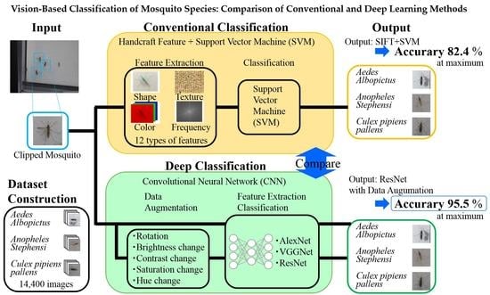
In this study, we considered the mosquito species classification method. This study aimed to compare the handcraft feature-based conventional classification method and CNN-based deep learning method. By comparing the accuracy of the two aforementioned methods, we observed an effective method for identifying mosquito species, thereby improving the recognition accuracy.

The rest of this study is organized as follows. Section 2 constructs the mosquito dataset and Section 3 explains the conventional and deep learning classification methods. The experimental verification and additional experimental validation are presented in Section 4 and Section 5, respectively. Section 6 summarizes the main contributions of our study.

2. Dataset Construction

This section describes the preconditions and the dataset construction.

As discussed in the introduction, Aedes, Anopheles, and Culex are the human blood-sucking mosquitoes. The most infectious species among the Aedes genus are Aedes albopictus and Aedes aegypti. The most infectious species among the Anopheles genus is Anopheles stephensi. The most infectious species among the Culex genus is Culex pipiens pallens.

The time zone, behavior habits, and infectious diseases of Aedes albopictus and Aedes aegypti are similar. Experts may find challenges in determining the difference in appearance even with the aid of a microscope. Therefore, we targeted Aedes albopictus out of the two species because of its large global population.

We utilized the images obtained by using a single-lens reflex camera to learn, while images obtained using a smartphone were used for testing and further validation. In addition, we assumed that the illuminance varied from 380 to 1340 lx and the background was white herein.

Table 1. Shooting equipment characteristics.

	Single-Lens Reflex Camera	Smartphone
Product name	EOS kiss X8i (Canon)	iPhone6S (Apple)
Picture size [pixel]	6000 × 4000	4032 × 3024
Resolution [dpi]	72 × 72	72 × 72
Lens model	EF-S18-55 mm F3.5-5.6 IS STM (Canon)	–
Focal length [mm]	3.5–5.6	2.2

presents the details of the shooting equipment. Figure 1 depicts an example of the captured images. The region of the mosquito was manually clipped from the captured images. Figure 2 and Figure 3 demonstrate the clipped mosquitoes from the images captured using a single-lens reflex camera and a smartphone, respectively.

Each clipped image was rotated by 90°, and all the rotated images were added to the dataset; the number of images had a four-fold increase. Consequently, we obtained the images of each mosquito species, consisting of 4000 images for training, 500 images for testing, and 300 images for validating. In general, the dataset with three types of mosquitoes comprised 12,000 images for training, 1500 images for testing, and 900 images for validating.

3. Classification Method

Figure 4 illustrates the system flow. We constructed a dataset of mosquito species and conducted a classification using handcraft features or deep learning. The classifications using handcraft features and classification using deep learning are hereinafter referred to as conventional classification and deep classification, respectively.

3.1. Conventional Classification

In this section, we present the details of conventional classification. Twelve types of handcraft features, including shape, color, texture, and frequency, were adopted for handcraft feature extraction and the SVM method was adopted for classification.

For the shape features, we extracted speeded-up robust features (SURF) [8], scale-invariant feature transform (SIFT) [9], dense SIFT [10], histogram of oriented gradients (HOG) [11], co-occurrence HOG (CoHOG) [12], extended CoHOG (ECoHOG) [13], and local binary pattern (LBP) [14]. SURF and SIFT comprised of two algorithms of feature point detection and feature description. Feature point detection is robust with respect to the changing scale and noise, and feature description is robust with respect to illumination change and rotation. Dense SIFT uses a grid pattern for feature points and denotes the same feature description as that denoted by SIFT. An example of the detected key point is depicted in Figure 5. The features extracted from SURF, SIFT, and dense SIFT were respectively clustered using k-means and vector quantization, conducted using a bag-of-features [15]. HOG is a histogram of the luminance gradient, and CoHOG is a histogram of the appearance frequency of a combination of the luminance gradients. ECoHOG is a histogram of the intensity of a combination of the luminance gradients. The LBP transforms into an LBP image that is robust to illumination change and exhibits its luminance histogram.

As the color features, we calculated color histograms in each colorimetric systems of red, green, blue (RGB), hue, saturation, value (HSV), and L * a * b * [16]. The RGB color system uses a simple concatenation of R, G, and B channel histograms. HSV is a color feature that uses the HSV color specification system; when the color saturation is low in the HSV color system, the hue value becomes unstable. Therefore, the histogram of each channel excludes the value when the saturation value is 10% or less. L * a * b * is a color feature that uses the L * a * b * color system and a three-dimensional histogram of L *, a *, b *.

For the texture features, we calculated a co-occurrence matrix feature (GLCM: gray level co-occurrence matrix). We used contrast, dissimilarity, homogeneity, energy, correlation, and angular secondary moment as the statistical values of GLCM [17].

For the frequency features, we utilized GIST [18], which is characterized by imitating human perception. GIST divides the image into small 4 × 4 blocks and extracts the structure of the entire image using filters with different frequencies and scales.

Classification of the mosquito species was conducted using SVM and the aforementioned features. SVM considered a soft margin, and multiclass classification was performed using a one-versus-rest method.

3.2. Deep Classification

In this section, we give the details of the CNN-based deep classification. Three types of architectures, including AlexNet [19], Visual Geometry Group Network (VGGNet) [20], and Deep residual network (ResNet) [21], were adopted for classification.

These architectures are often used for object recognition. AlexNet was used as it has been proposed. Note that VGGNet uses 16 layers of network and that ResNet uses 18 layers of network structure.

The CNN learning method was conducted using a stochastic gradient descent method, and the learning rate schedule was obtained using simulated annealing. The ImageNet pre-trained weights [22] were used as initial weights to accelerate the convergence of learning.

As explained in Section 2, we captured mosquito images with a simple white background. Images with the little-noised simple background can lead to overfitting images for training and a declined generality.

To suppress overfitting, the training images were transformed by the following data augmentation steps.

• Rotation: Rotate the image by angle $\theta$.
  Angle $\theta$ varies randomly in the range from −${\theta }_r$ to ${\theta }_r$.
  Here, the limit value ${\theta }_r$ is set to be 45°.
• Brightness change: Randomly change the brightness of the image.
  Change rate $\alpha$ is chosen in the range from −${\alpha }_r$ to ${\alpha }_r$.
  Here, the limit value ${\alpha }_r$ is set to be 40%.
• Contrast change: Randomly change the contrast of the image.
  Change rate $\alpha$ is chosen in the range from −${\alpha }_r$ to ${\alpha }_r$.
  Here, the limit value ${\alpha }_r$ is set to be 40%.
• Saturation change: Randomly change the saturation of the image.
  Change rate $\alpha$ is chosen in the range from −${\alpha }_r$ to ${\alpha }_r$.
  Here, the limit value ${\alpha }_r$ is set to be 40%.
• Hue change: Randomly change the hue of the image.
  Change rate $\alpha$ is chosen in the range from −${\alpha }_r$ to ${\alpha }_r$.
  Here, the limit value ${\alpha }_r$ is set to be 25%.

The limit values, ${\theta }_r$ and ${\alpha }_r$, were determined a priori by reference to the default ones used in the iNaturalist Competition 2018 Training Code. It is noteworthy that the number of training images was constant since the transformed image was replaced by the original one.

An example of the data augmentation is depicted in Figure 6. The variation of training images increases in terms of color, brightness, and rotation fluctuation based on the aforementioned processing.

4. Mosquito Species Classification Experiment

4.1. Experimental Conditions

The mosquitoes were classified using the dataset presented in Section 2. We used Aedes albopictus, Anopheles stefensi, and Culex pipiens pallens as species classification targets. The images captured using a single-lens reflex camera were used for training, and the images captured using a smartphone were used for the test. We used the dataset with three types of mosquitoes consisting of 12,000 images for training and 1500 images for testing. In the case of the deep classification, training and testing phases were performed five times, and the average classification accuracy was calculated.

4.2. Experimental Results

Table 2. Result of conventional classification. Speeded-up robust features (SURF); histogram of oriented gradient (HOG); co-occurrence HOG (CoHOG); extended CoHOG (ECoHOG); local binary pattern (LBP); red, green, blue (RGB); hue, saturation, value (HSV); gray level co-occurrence matrix (GLCM); GIST. L*a*b*.

Features	Accuracy [%]	Features	Accuracy [%]
SURF	81.6	LBP	57.3
SIFT	82.4	RGB	30.7
Dense SIFT	55.9	HSV	37.4
HOG	54.7	L*a*b*	33.7
CoHOG	57.0	GLCM	53.6
ECoHOG	61.1	GIST	71.5

and

Table 3. Result of deep classification. AlexNet; Visual Geometry Group Network (VGGNet); Deep residual network (ResNet).

Architecture	Accuracy [%]
	Data Augmentation
		✓
AlexNet	69.8	92.3
VGGNet	81.2	91.0
ResNet	74.4	95.5

show the aggregated accuracies over the three considered species of conventional and deep classifications, respectively.

In conventional classification, parameters for features were set to default values adopted in OpenCV libraries on Python. The hyperparameters of SVM were determined based on preliminary experiments. The error-term penalty parameter, C, was set to one and the kernel function was defined as a linear kernel. The SVM classifier with these parameters had the highest accuracy in the grid search.

The classification accuracies with SIFT and SURF are high. By applying the fact that the classification with dense SIFT exhibits low accuracy, it turns out that an algorithm that detects feature points and describes local features is effective.

The deep classification has a lower classification accuracy than the conventional classification unless it is by data augmentation. By applying data augmentation, the deep classification has higher accuracy than the conventional classification. Therefore, data augmentation is effective. ResNet has the highest discrimination accuracy of 95.5%, indicating that deep classification is effective for mosquito species classification.

Figure 7 shows the confusion matrices. Figure 7a shows one from the conventional classification with SIFT, which achieved the highest accuracy in Table 2. Each species is misclassified from each other in comparison with the deep classification result.

Figure 7b shows one from the deep classification with ResNet, which achieved the highest accuracy in Table 3. This matrix was calculated from the result of one training and testing phase among five ones. Aedes albopictus and Culex pipiens pallens are relatively misclassified as each other, whereas Anopheles stefensi is relatively classified appropriately.

Figure 8 shows an image visualizing the target spot in gradient-weighted class activation mapping (Grad-CAM), which is a visualization method [23] for deep classification. The heatmap covers the body of the mosquito.

Aedes albopictus and Culex pipiens pallens have a similar shape but their body colors are different. Nevertheless, Aedes albopictus and Culex pipiens pallens can be classified based on similar body parts from the visualization result. The images captured using a smartphone do not indicate the color differences when the shooting environment is dark because a smartphone camera is unable to offer a quality shot when compared with the single-lens reflex cameras. The above facts lead to misclassification.

5. Effective Data Augmentation Investigation Experiment

We showed that the deep classification achieves a higher classification accuracy by data augmentation in Section 4. In this section, as further validation, we investigated which transformation step of the data augmentation is effective for deep classification.

5.1. Experimental Conditions

As explained in Section 3.2, we applied transformation steps to the training images for data augmentation. However, it is not clear which step contributes the most to the classification. In addition, the range values, ${\theta }_r$ and ${\alpha }_r$, were determined a priori.

By the data augmentation described in Section 3.2, we verified the step which contributes the most to the classification accuracy.

In this experiment, we chose one transformation step from the steps explained in Section 3.2 and applied the chosen transformation separately to the training images.

• Rotation: rotate the image by angle $\theta$.
  Angle $\theta$ varies randomly in the range from −${\theta }_r$ to ${\theta }_r$.
• Brightness change: Randomly change the brightness of the image.
  Change rate $\alpha$ is chosen in the range from −${\alpha }_r$ to ${\alpha }_r$.
• Contrast change: Randomly change the contrast of the image.
  Change rate $\alpha$ is chosen in the range from −${\alpha }_r$ to ${\alpha }_r$.
• Saturation change: Randomly change the saturation of the image.
  Change rate $\alpha$ is chosen in the range from −${\alpha }_r$ to ${\alpha }_r$.
• Hue change: Randomly change the hue of the image.
  Change rate $\alpha$ is chosen in the range from −${\alpha }_r$ to ${\alpha }_r$.

Regarding rotation, the limit value ${\theta }_r$ varied at 5° intervals from 0° to 45°. Therefore, the 10 conditions were prepared. Conditions A to J denote the ranges of angle $\theta$; [0 (no rotation,${\theta }_r$ = 0)], [−5 to 5 (${\theta }_r$ = 5)], …, [−45 to 45 (${\theta }_r$ = 45)], respectively.

Regarding the brightness, contrast, saturation, or hue change, the limit value ${\alpha }_r$ varied at five intervals from 0% to 50%. Therefore, the 11 by 4 conditions were prepared. Conditions A to K denote the ranges of change rate α; [0 (no change, α_r = 0)], [−5 to 5 (α_r = 5)], …, [−50 to 50 α_r = 50)], respectively.

We utilized the dataset with three types of mosquitoes, comprising 12,000 images for training and 900 images for validation. Training and validation were performed five times by considering each condition, and the average of classification accuracy was calculated. Generally, 270 (54 conditions by five trials) trials of training and validation were performed.

5.2. Experimental Results

Figure 9 shows the experimental results. The error bar shows the standard deviation.

Regarding rotation, the classification accuracy is almost the same at any condition. As mentioned in Section 2, the clipped training image was rotated by 90°, and all the rotated images were added to the dataset. We observed that the rotation variation seems to be retained in advance; hence, the rotation has small effects on the accuracy in this experiment that we conducted.

Regarding brightness, saturation, or hue changes, the accuracy improves up to the condition E (${\alpha }_r$ = 25) or G (α_r = 30), and there are little changes afterward.

Regarding contrast change, the accuracy improves with the increase in the change rate. In condition K(α_r = 50) of contrast, the highest classification accuracy achieved is 89.1%.

From the above, the fluctuation of contrast offers the most improvement in terms of the accuracy of mosquito species classification.

6. Conclusions

This study compared the handcraft feature-based conventional classification method and CNN-based deep classification method. We constructed a dataset for classifying mosquito species. For conventional classification, shape, color, texture, and frequency were adopted for handcraft feature extraction, and the SVM method was adopted for classification. For deep classification, three types of architectures were adopted and compared.

The deep classification had a lower classification accuracy than the conventional classification unless by data augmentation. However, by data augmentation, deep classification had a higher accuracy than the conventional classification. ResNet achieved the highest discrimination accuracy of 95.5%, indicating that deep classification is effective for mosquito species classification. Furthermore, we verified that data augmentation with the fluctuation of contrast contributes the most improvement.

References

- World Health Organization: Mosquito-Borne Diseases. Available online: http://www.who.int/neglected_diseases/vector_ecology/mosquito-borne-diseases/en/ (accessed on 1 April 2017).
- Fuchida, M.; Pathmakumar, T.; Mohan, R.E.; Tan, N.; Nakamura, A. Vision-based perception and classification of mosquitoes using support vector machine. Appl. Sci. 2017, 7, 51. [Google Scholar] [CrossRef]
- Minakshi, M.; Bharti, P.; Chellappan, S. Identifying mosquito species using smart-phone camera. In Proceedings of the 2017 European Conference on Networks and Communications (EuCNC), Oulu, Finland, 12–15 June 2017. [Google Scholar]
- Nilsback, M.E.; Zisserman, A. Automated flower classification over a large number of classes. In Proceedings of the 2008 Sixth Indian Conference on Computer Vision, Graphics & Image Processing (ICVGIP), Bhubaneswar, India, 16–19 December 2008. [Google Scholar]
- Welinder, P.; Branson, S.; Mita, T.; Wah, C.; Schroff, F.; Belongie, S.; Perona, P. Caltech-UCSD Birds 200. In Technical Report CNS-TR-2010-001; California Institute of Technology: Pasadena, CA, USA, 2010. [Google Scholar]
- Hou, S.; Feng, Y.; Wang, Z. VegFru: A domain-specific dataset for fine-grained visual categorization. In Proceedings of the IEEE International Conference on Computer Vision (ICCV), Venice, Italy, 22–29 October 2017. [Google Scholar]
- Horn, G.V.; Aodha, O.M.; Song, Y.; Cui, Y.; Sun, C.; Shepard, A.; Adam, H.; Perona, P.; Belongie, S. The inaturalist species classification and detection dataset. In Proceedings of the IEEE Conference on Computer Vision and Pattern Recognitionin, Salt Lake City, UT, USA, 18–22 June 2018. [Google Scholar]
- Bay, H.; Tuytelaars, T.; Gool, L.V. SURF: Speeded up robust features. In Proceedings of the European Conference on Computer Vision (ECCV), Amsterdam, The Netherlands, 8–16 October 2006. [Google Scholar]
- Lowe, D.G. Distinctive image features from scale-invariant keypoints. Int. J. Comp. Vis. 2004, 60, 91–110. [Google Scholar] [CrossRef]
- Liu, C.; Yuen, J.; Torralba, A.; Sivic, J.; Freeman, W.T. SIFT flow: Dense correspondence across different scenes. In Proceedings of the European Conference on Computer Vision (ECCV), Marseille, France, 12–18 October 2008. [Google Scholar]
- Dalal, N.; Triggs, B. Histogram of oriented gradients for human detection. In Proceedings of the International Conference on Computer Vision and Pattern Recognition (CVPR), San Diego, CA, USA, 20–25 June 2005. [Google Scholar]
- Watanabe, T.; Ito, S.; Yokoi, K. Co-occurrence histograms of oriented gradients for pedestrian detection. In Proceedings of the Pacific-Rim Symposium on Image and Video Technology (PSIVT), Tokyo, Japan, 13–16 January 2009. [Google Scholar]
- Kataoka, H.; Aoki, Y. Symmetrical judgment and improvement of CoHOG feature descriptor for pedestrian detection. In Proceedings of the Machine Vision Applications (MVA), Nara, Japan, 13–15 June 2011. [Google Scholar]
- Ojala, T.; Pietikainen, M.; Harwood, D. A comparative study of texture measures with classification based on feature distributions. Pattern Recognit. 1996, 29, 51–59. [Google Scholar] [CrossRef]
- Csurka, G.; Dance, C.R.; Fan, L.; Willamowski, J.; Bray, C. Visual categorization with bags of keypoints. In Proceedings of the European Conference on Computer Vision (ECCV), Prague, Czech Republic, 11–14 May 2004. [Google Scholar]
- Palermo, F.; Hays, J.; Efros, A.A. Dating historical color images. In Proceedings of the European Conference on Computer Vision (ECCV), Florence, Italy, 7–13 October 2012. [Google Scholar]
- Haralick, R.M.; Shanmugam, K. Textural features for image classification. IEEE Trans. Syst. Man Cybernet. 1973, 610–621. [Google Scholar] [CrossRef]
- Oliva, A.; Torralba, A. Modeling the shape of the scene: A holistic representation of the spatial envelope. Int. J. Comp. Vis. 2001, 3, 145–175. [Google Scholar] [CrossRef]
- Krizhevsky, A.; Sutskever, I.; Hinton, G.E. Imagenet classification with deep convolutional neural networks. In Proceedings of the Advances in Neural Information Processing Systems (NIPS), Lake Tahoe, NV, USA, 3–6 December 2012. [Google Scholar]
- Simonyan, K.; Zisserman, A. Very deep convolutional networks for large-scale image recognition. In Proceedings of the International Conference on Learning Representations (ICLR), San Diego, CA, USA, 7–9 May 2015. [Google Scholar]
- He, K.; Zhang, X.; Ren, S.; Sun, J. Deep residual learning for image recognition. In Proceedings of the IEEE Conference on Computer Vision and Pattern Recognition (CVPR), Las Vegas, NV, USA, 27–30 June 2016. [Google Scholar]
- He, K.; Girshick, R.; Dollar, P. Rethinking imagenet pre-training. arXiv 2018, arXiv:1811.08883. [Google Scholar]
- Selvaraju, R.R.; Cogswell, M.; Das, A.; Vedantam, R.; Parikh, D.; Batra, D. Grad-CAM: Visual explanations from deep networks via gradient-based localization. In Proceedings of the IEEE International Conference on Computer Vision (ICCV), Venice, Italy, 22–29 October 2017. [Google Scholar]
Figure 1.
Examples of the captured images: (a) Mosquitoes captured using a single-lens reflex camera and (b) mosquitoes captured using a smartphone.
Figure 2.
Clipped mosquitoes from the images captured using a single-lens reflex camera: (a) Aedes albopictus, (b) Anopheles stephensi, and (c) Culex pipiens pallens.
Figure 3.
Clipped mosquito from the images captured using a smartphone: (a) Aedes albopictus, (b) Anopheles stephensi, and (c) Culex pipiens pallens.
Figure 5.
Visualization of keypoint detection: (a) Speeded-up robust features (SURF), (b) scale-invariant feature transform (SIFT), and (c) dense SIFT.
Figure 6.
Examples of data argumentation.
Figure 7.
Example results of the confusion matrices.
Figure 8.
Activation visualization by gradient-weighted class activation mapping (Grad-CAM): (a) Aedes albopictus, (b) Anopheles stephensi, and (c) Culex pipiens pallens.
Figure 9.
Classification accuracy due to variations in the data argumentation steps: (a) rotation, (b) brightness change, (c) contrast change, (d) saturation change, and (e) hue change.