Improving the Reliability of Photovoltaic and Wind Power Storage Systems Using Least Squares Support Vector Machine Optimized by Improved Chicken Swarm Algorithm

 ,
,
Abstract
:1. Introduction
2. Lifetime Prediction Model for Lithium-Ion Batteries
2.1. Least Squares Support Vector Machine(LSSVM) Principle
2.2. The Particle Swarm Optimization (PSO) Algorithm
2.3. The Chicken Swarm Optimization Algorithm (CSO)
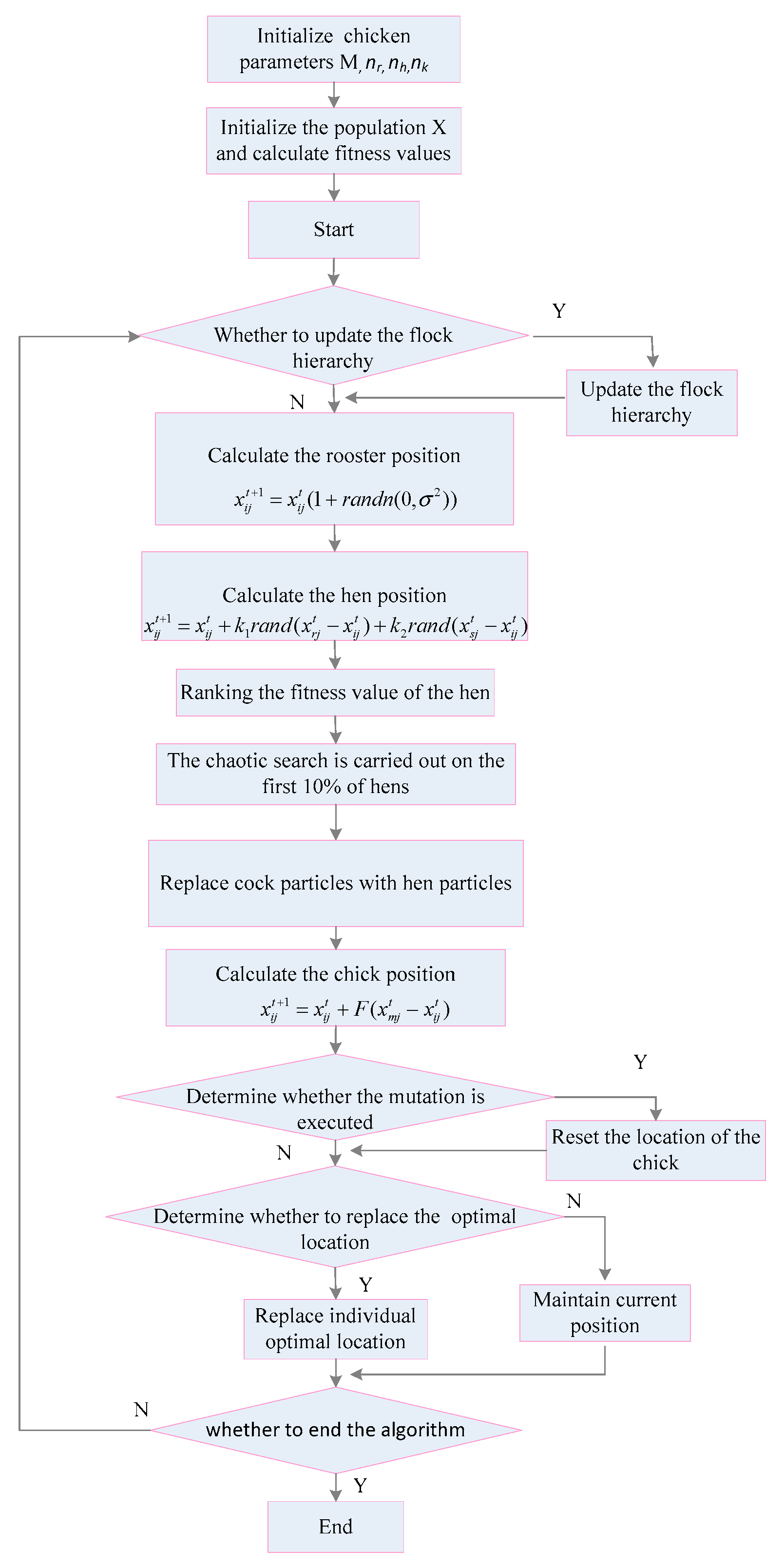
2.4. The Improved Chicken Swarm Optimization Algorithm (ICSO)
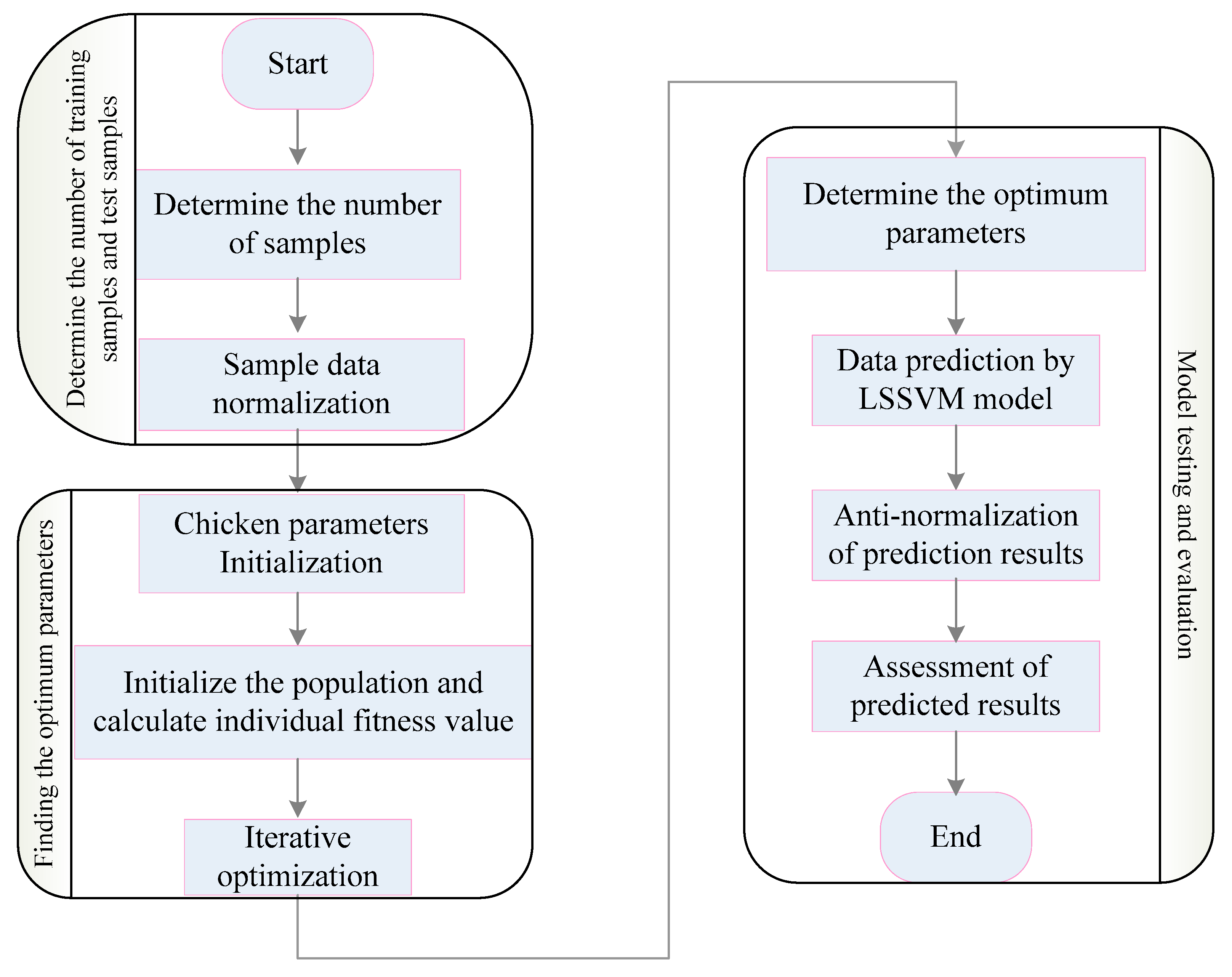
2.5. ICSO-LSSVM Model
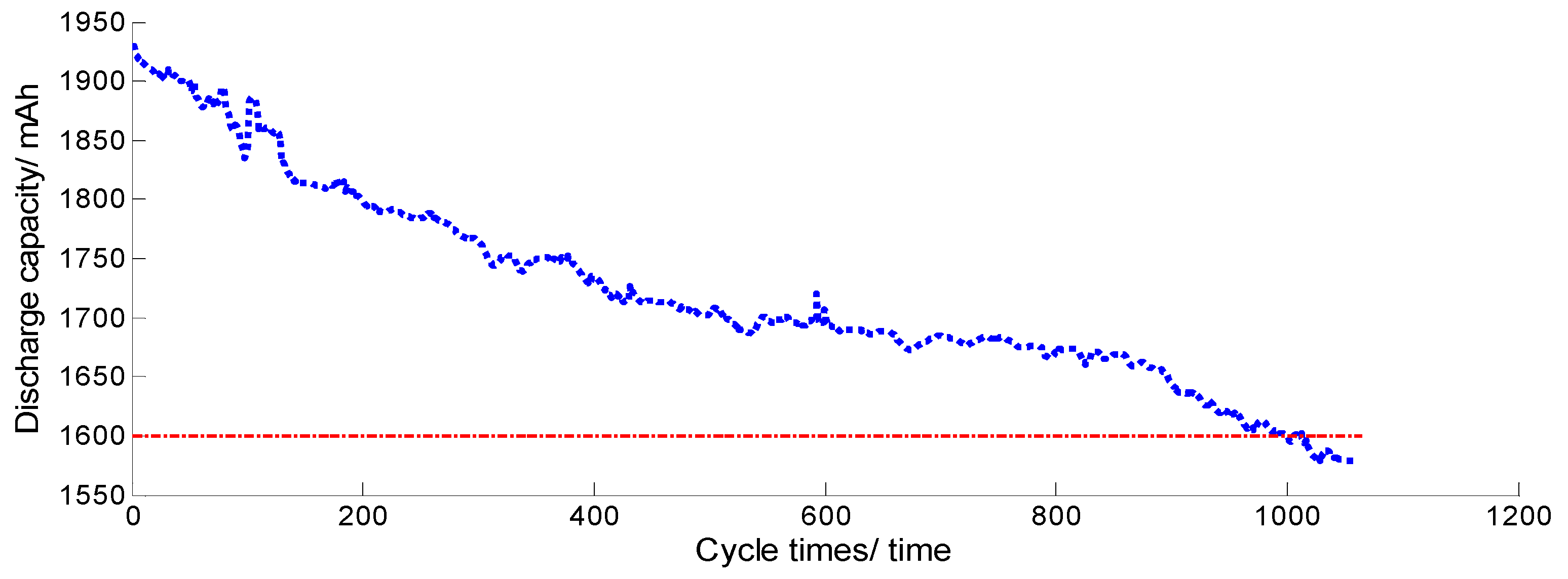
3. Charge and Discharge Test
4. Test Simulation and Result Analysis
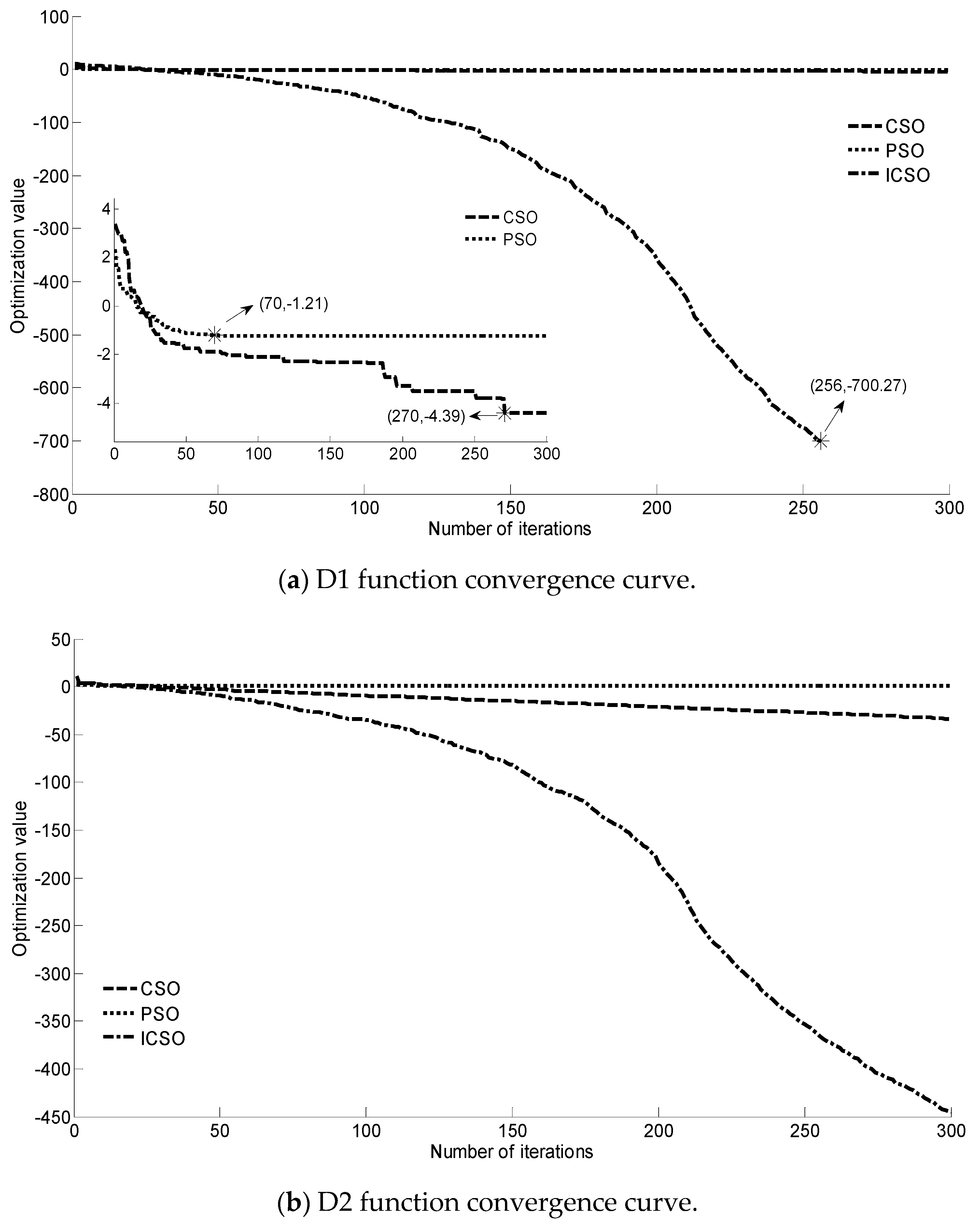
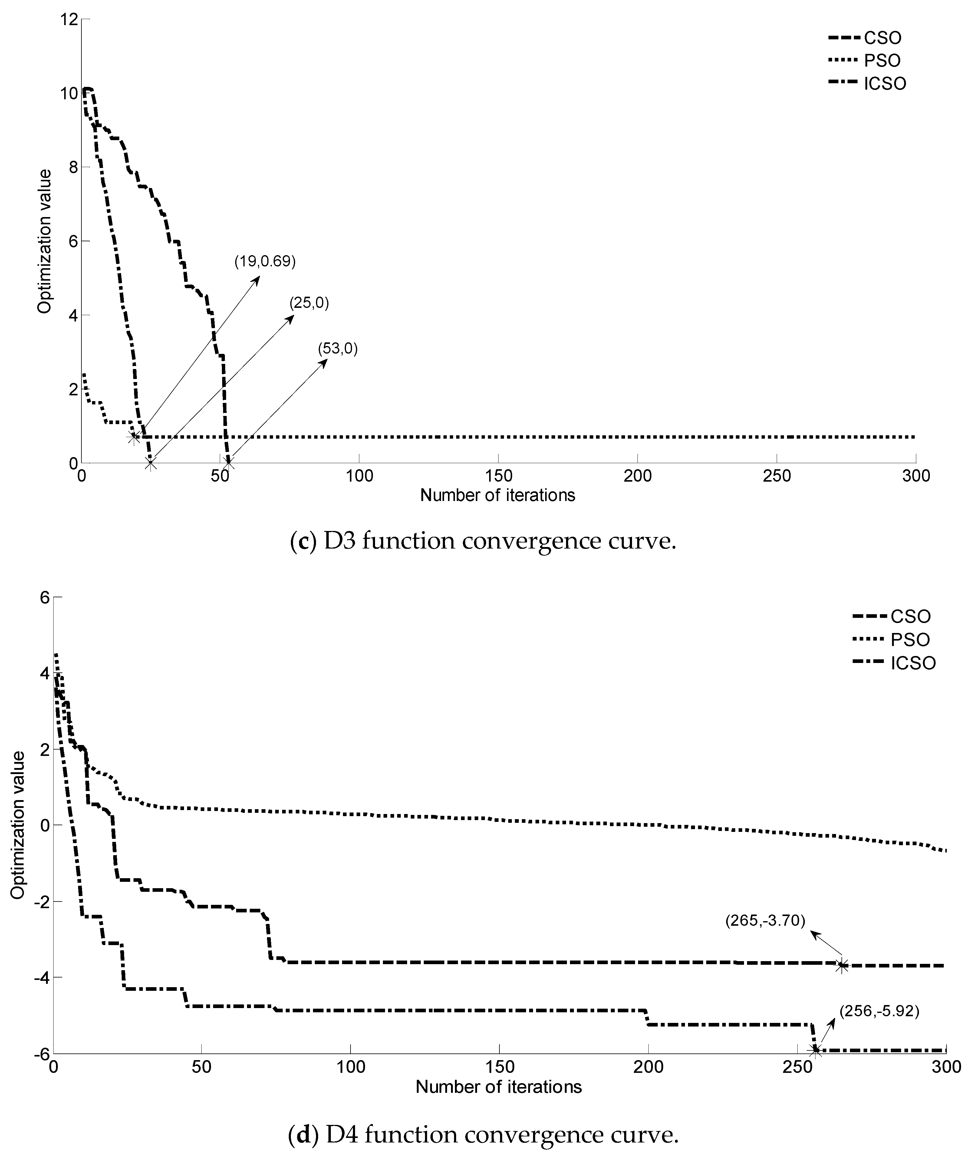
4.1. Analysis of Algorithm Convergence Performance
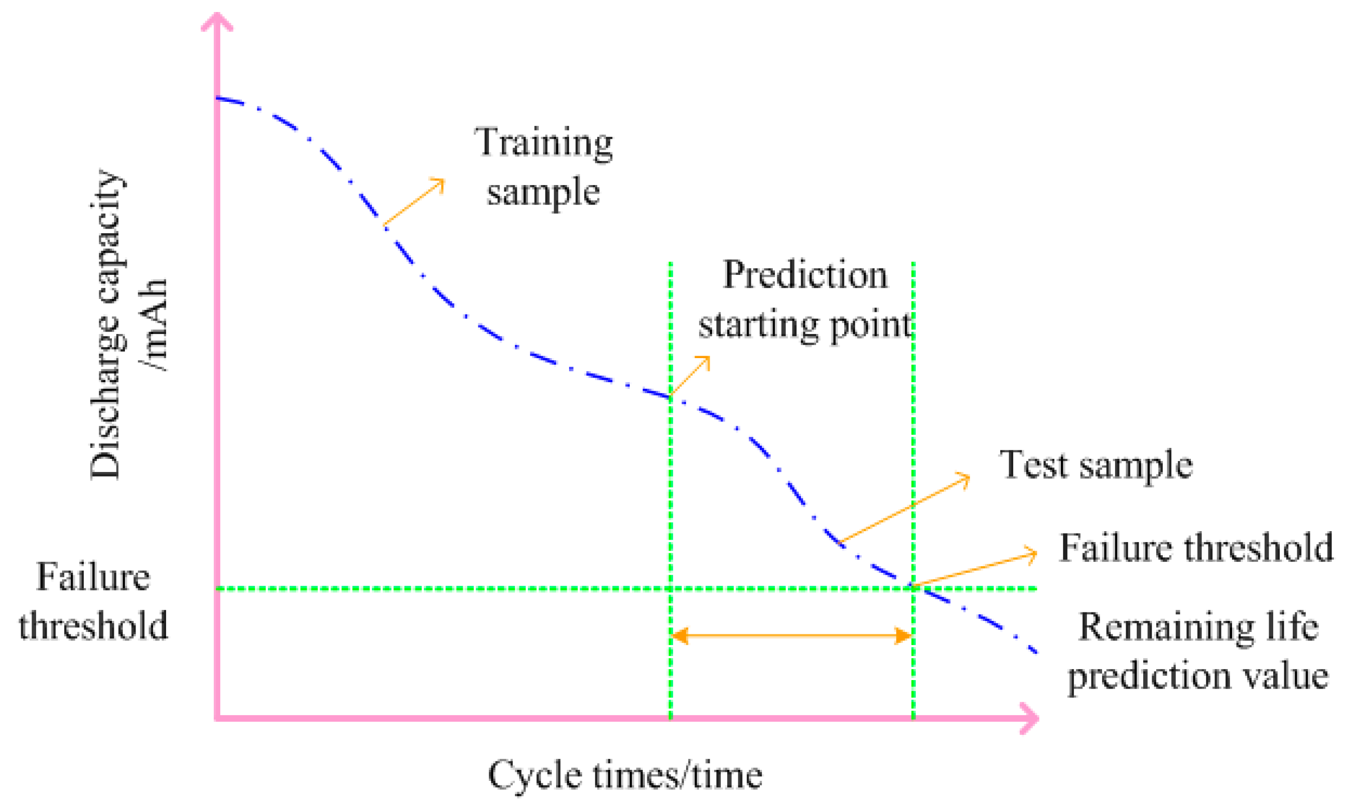
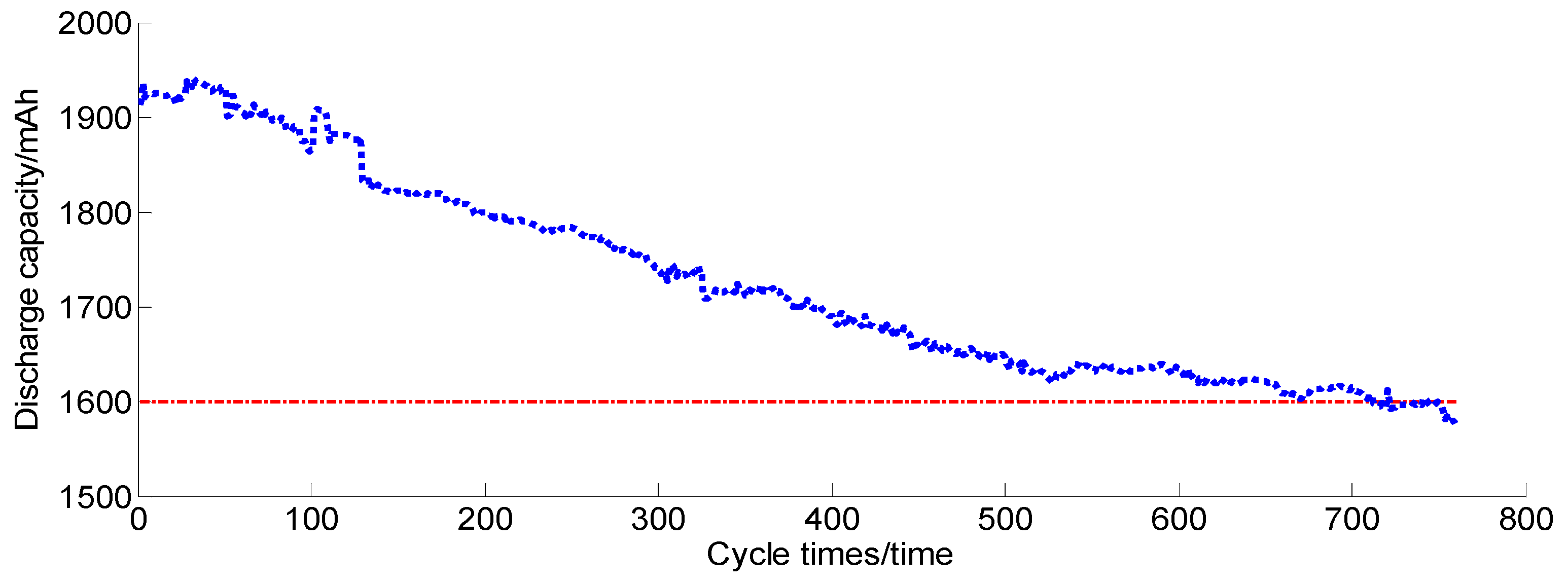
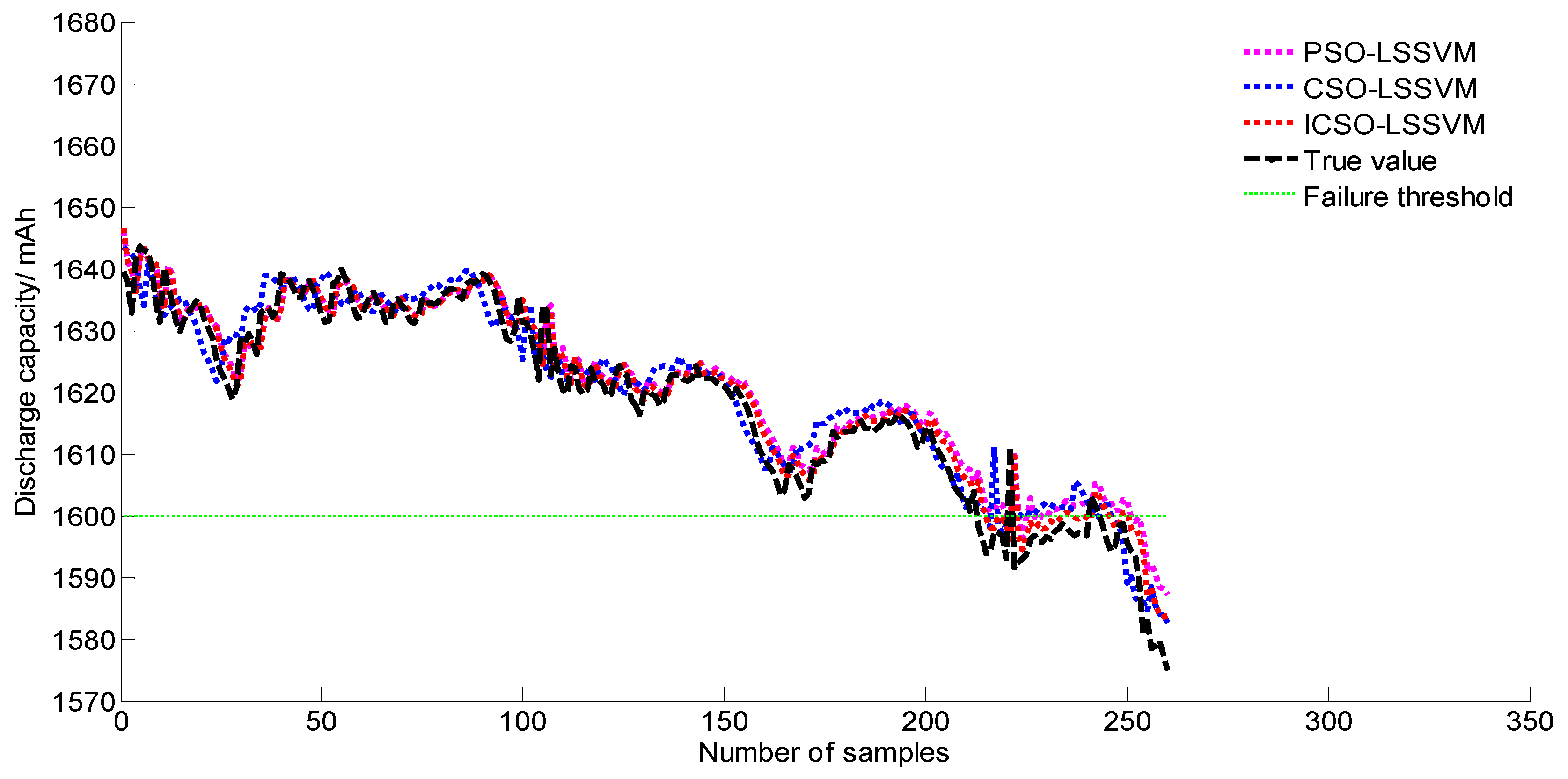
4.2. Simulation Experiment on Life Prediction of Lithium-Ion Battery
5. Conclusions
Author Contributions
Funding
Acknowledgments
Conflicts of Interest
References
- Wang, Y.P.; Li, J. Spatial Spillover Effect of Non-Fossil Fuel Power Generation on Carbon Dioxide Emissions across China’s Provinces. Renew. Energy 2019, 136, 317–330. [Google Scholar] [CrossRef]
- Mamat, R.; Sani, M.S.M.; Sudhakar, K. Renewable Energy in Southeast Asia: Policies and Recommendations. Sci. Total Environ. 2019, 670, 1095–1102. [Google Scholar]
- Jiaqiang, E.; Zhang, Z.; Tu, Z.; Zuo, W.; Hu, W.; Han, D.; Jin, Y. Effect analysis on flow and boiling heat transfer performance of cooling water-jacket of bearing in the gasoline engine turbocharger. Appl. Therm. Eng. 2018, 130, 754–766. [Google Scholar]
- Deng, Y.; Liu, H.; Zhao, X.; Jiaqiang, E.; Chen, J. Effects of cold start control strategy on cold start performance of the diesel engine based on a comprehensive preheat diesel engine model. Appl. Energy 2018, 210, 279–287. [Google Scholar] [CrossRef]
- Zhang, Z.; Jiaqiang, E.; Deng, Y.; Zuo, W.; Peng, Q.; Hieu, P.; Yin, Z. Effects of fatty acid methyl esters proportion on combustion and emission characteristics of a biodiesel fueled marine diesel engine. Energy Convers. Manag. 2018, 159, 244–253. [Google Scholar] [CrossRef]
- Zhang, B.; Jiaqiang, E.; Gong, J.; Yuan, W.; Zuo, W.; Li, Y.; Fu, J. Multidisciplinary design optimization of the diesel particulate filter in the composite regeneration process. Appl. Energy 2016, 181, 14–28. [Google Scholar] [CrossRef]
- Zhang, B.; Jiaqiang, E.; Gong, J.; Yuan, W.; Zhao, X.; Hu, W. Influence of structural and operating factors on performance degradation of the diesel particulate filter based on composite regeneration. Appl. Therm. Eng. 2017, 121, 838–852. [Google Scholar] [CrossRef]
- Ashuri, T.; Zaaijer, M.B.; Martins, J.; van Bussel, G.J.W.; van Kuik, G.A.M. Multidisciplinary design optimization of offshore wind turbines for minimum levelized cost of energy. Renew. Energy 2014, 68, 893–905. [Google Scholar] [CrossRef] [Green Version]
- Jiaqiang, E.; Zuo, W.; Gao, J.; Peng, Q.; Zhang, Z.; Hieu, P. Effect analysis on pressure drop of the continuous regeneration-diesel particulate filter based on NO2 assisted regeneration. Appl. Therm. Eng. 2016, 100, 356–366. [Google Scholar]
- Chen, M.R.; Zeng, G.Q.; Lu, K.D. Constrained multi-objective population extremal optimization based economic-emission dispatch incorporating renewable energy resources. Renew. Energy 2019, 143, 277–294. [Google Scholar] [CrossRef]
- Ye, B.; Yang, P.; Jiang, J.J.; Miao, L.X.; Shen, B.; Li, J. Feasibility and economic analysis of a renewable energy powered special town in China. Resour. Conserv. Recycl. 2017, 121, 40–50. [Google Scholar] [CrossRef]
- Solomon, A.A.; Kammen, D.M.; Callaway, D. Investigating the impact of wind-solar complementarities on energy storage requirement and the corresponding supply reliability criteria. Appl. Energy 2016, 168, 130–145. [Google Scholar] [CrossRef]
- Du, W.; Bi, J.; Lv, C.; Littler, T. Damping torque analysis of power systems with DFIGs for wind power generation. IET Renew. Power Gener. 2017, 11, 10–19. [Google Scholar] [CrossRef]
- Hill, C.A.; Such, M.C.; Chen, D.; Gonzalez, J.; Grady, W.M. Battery Energy Storage for Enabling Integration of Distributed Solar Power Generation. IEEE Trans. Smart Grid 2012, 3, 850–857. [Google Scholar] [CrossRef]
- Ma, X.; Qiu, D.F.; Tao, Q.; Zhu, D.Y. State of Charge Estimation of a Lithium Ion Battery Based on Adaptive Kalman Filter Method for an Equivalent Circuit Model. Appl. Sci. Basel 2019, 9, 2765. [Google Scholar] [CrossRef]
- Liu, Y.; Wang, H.C.; Yang, K.K.; Yang, Y.N.; Ma, J.Q.; Pan, K.M.; Pang, H. Enhanced Electrochemical Performance of Sb2O3 as an Anode for Lithium-Ion Batteries by a Stable Cross-Linked Binder. Appl. Sci. Basel 2019, 9, 2677. [Google Scholar] [CrossRef]
- Tian, L.L.; Wang, M.K.; Xiong, L.; Guo, H.J.; Huang, C.; Zhang, H.R.; Chen, X.D. The Effect of Different Mixed Organic Solvents on the Properties of p(OPal-MMA) Gel Electrolyte Membrane for Lithium Ion Batteries. Appl. Sci. Basel 2018, 8, 2587. [Google Scholar] [CrossRef]
- Jaguemont, J.; Boulon, L.; Venet, P.; Dubé, Y.; Sari, A. Lithium-Ion Battery Aging Experiments at Subzero Temperatures and Model Development for Capacity Fade Estimation. IEEE Trans. Veh. Technol. 2016, 65, 4328–4343. [Google Scholar] [CrossRef]
- Richa, K.; Babbitt, C.W.; Gaustad, G.; Wang, X. A future perspective on lithium-ion battery waste flows from electric vehicles. Resour. Conserv. Recycl. 2014, 83, 63–76. [Google Scholar] [CrossRef]
- Wang, D.; Yang, F.; Tsui, K.-L.; Zhou, Q.; Bae, S.J. Remaining Useful Life Prediction of Lithium-Ion Batteries Based on Spherical Cubature Particle Filter. IEEE Trans. Instrum. Meas. 2016, 65, 1282–1291. [Google Scholar] [CrossRef]
- Waag, W.; Kabitz, S.; Sauer, D.U. Experimental investigation of the lithium-ion battery impedance characteristic at various conditions and aging states and its influence on the application. Appl. Energy 2013, 102, 885–897. [Google Scholar] [CrossRef]
- Sanchez, L.; Couso, I.; Gonzalez, M. A design methodology for semi-physical fuzzy models applied to the dynamic characterization of LiFePO4 batteries. Appl. Soft Comput. 2014, 14, 269–288. [Google Scholar] [CrossRef]
- Sbarufatti, C.; Corbetta, M.; Giglio, M.; Cadini, F. Adaptive prognosis of lithium-ion batteries based on the combination of particle filters and radial basis function neural networks. J. Power Sources 2017, 344, 128–140. [Google Scholar] [CrossRef]
- Gao, D.; Huang, M.H. Prediction of Remaining Useful Life of Lithium-ion Battery based on Multi-kernel Support Vector Machine with Particle Swarm Optimization. J. Power Electron. 2017, 17, 1288–1297. [Google Scholar]
- Wang, Z.P.; Ma, J.; Zhang, L. State-of-Health Estimation for Lithium-Ion Batteries Based on the Multi-Island Genetic Algorithm and the Gaussian Process Regression. IEEE Access 2017, 5, 21286–21295. [Google Scholar] [CrossRef]
- Andre, D.; Nuhic, A.; Soczka-Guth, T.; Sauer, D.U. Comparative study of a structured neural network and an extended Kalman filter for state of health determination of lithium-ion batteries in hybrid electric vehicles. Eng. Appl. Artif. Intell. 2013, 26, 951–961. [Google Scholar] [CrossRef]
- Gao, Y.Z.; Zhang, X.; Yang, J.; Guo, B.J.; Zhou, X. A Novel Model for Lithium-Ion Battery Aging Quantitative Analysis Based on Pseudo Two-Dimension Expressions. Int. J. Electrochem. Sci. 2019, 14, 3180–3203. [Google Scholar] [CrossRef]
- Zhang, Y.Z.; Xiong, R.; He, H.W.; Pecht, M. Validation and Verification of a Hybrid Method for Remaining Useful Life Prediction of Lithium-Ion Batteries. J. Clean. Prod. 2019, 212, 240–249. [Google Scholar] [CrossRef]
- Cortes, C.; Vapnik, V. Support-vector networks. Mach. Learn. 1995, 20, 273–297. [Google Scholar] [CrossRef]
- Suykens, J.A.K.; Vandewalle, J. Least squares support vector machine classifiers. Neural Process. Lett. 1999, 9, 293–300. [Google Scholar] [CrossRef]
- Liu, J.X.; Jia, Z.H. Telecommunication Traffic Prediction Based on Improved LSSVM. Int. J. Pattern Recognit. Artif. Intell. 2018, 32, 16. [Google Scholar] [CrossRef]
- Zheng, H.B.; Zhang, Y.Y.; Liu, J.F.; Wei, H.; Zhao, J.H.; Liao, R.J. A novel model based on wavelet LS-SVM integrated improved PSO algorithm for forecasting of dissolved gas contents in power transformers. Electr. Power Syst. Res. 2018, 155, 196–205. [Google Scholar] [CrossRef]
- Khelif, R.; Chebel-Morello, B.; Malinowski, S.; Laajili, E.; Fnaiech, F.; Zerhouni, N. Direct Remaining Useful Life Estimation Based on Support Vector Regression. IEEE Trans. Ind. Electron. 2017, 64, 2276–2285. [Google Scholar] [CrossRef]
- Al Shayokh, M.; Shin, S.Y. Bio Inspired Distributed WSN Localization Based on Chicken Swarm Optimization. Wirel. Pers. Commun. 2017, 97, 5691–5706. [Google Scholar] [CrossRef]
- Yu, X.W.; Zhou, L.X.; Li, X.Y. A Novel Hybrid Localization Scheme for Deep Mine Based on Wheel Graph and Chicken Swarm Optimization. Comput. Netw. 2019, 154, 73–78. [Google Scholar] [CrossRef]
- Biswal, P.C. Ancestor Approach to Number of Spanning Trees of Wheel Graph W-N in Terms of Number of Spanning Trees of Fan Graph F-N. Adv. Sci. Lett. 2016, 22, 567–569. [Google Scholar] [CrossRef]
- Zahid, A.; Saleem, M.U.; Kashif, A.; Khan, M.; Meraj, M.A.; Irfan, R. Spanning Simplicial Complex of Wheel Graph W-N. Algebra Colloq. 2019, 26, 309–320. [Google Scholar] [CrossRef]
- Datta, A.; Augustin, M.J.; Gupta, N.; Viswamurthy, S.R.; Gaddikeri, K.M.; Sundaram, R. Impact Localization and Severity Estimation on Composite Structure Using Fiber Bragg Grating Sensors by Least Square Support Vector Regression. IEEE Sens. J. 2019, 19, 4463–4470. [Google Scholar] [CrossRef]
- Wang, G.J.; Zhang, G.Q.; Choi, K.S.; Lu, J. Deep Additive Least Squares Support Vector Machines for Classification with Model Transfer. IEEE Trans. Syst. Man Cybern. Syst. 2019, 49, 1527–1540. [Google Scholar] [CrossRef]
- Shahsavar, A.; Bagherzadeh, S.A.; Mahmoudi, B.; Hajizadeh, A.; Afrand, M.; Nguyen, T.K. Robust Weighted Least Squares Support Vector Regression Algorithm to Estimate the Nanofluid Thermal Properties of Water/Graphene Oxide-Silicon Carbide Mixture. Phys. Stat. Mech. Appl. 2019, 525, 1418–1428. [Google Scholar] [CrossRef]
- Kennedy, J.; Eberhart, R. Particle swarm optimization. In Proceedings of the 1995 IEEE International Conference on Neural Networks, Perth, WA, Australia, 27 November–1 December 1995; Volume 4, pp. 1942–1948. [Google Scholar]
- Le, L.T.; Nguyen, H.; Zhou, J.; Dou, J.; Moayedi, H. Estimating the Heating Load of Buildings for Smart City Planning Using a Novel Artificial Intelligence Technique PSO-XGBoost. Appl. Sci. Basel 2019, 9, 2714. [Google Scholar] [CrossRef]
- Cheng, S.F.; Lu, F.; Peng, P.; Wu, S. Multi-Task and Multi-View Learning Based on Particle Swarm Optimization for Short-Term Traffic Forecasting. Knowl. Based Syst. 2019, 180, 116–132. [Google Scholar] [CrossRef]
- Almahdi, S.; Yang, S.Y. A Constrained Portfolio Trading System Using Particle Swarm Algorithm and Recurrent Reinforcement Learning. Expert Syst. Appl. 2019, 130, 145–156. [Google Scholar] [CrossRef]
- Gharebaghi, S.A.; Zangooei, E. Chaotic particle swarm optimization in optimal active control of shear buildings. Struct. Eng. Mech. 2017, 61, 347–357. [Google Scholar] [CrossRef]
- Chen, S.L.; Yang, R.Y.; Yang, R.H.; Yang, L.; Yang, X.Z.; Xu, C.B.; Liu, W.P. A Parameter Estimation Method for Nonlinear Systems Based on Improved Boundary Chicken Swarm Optimization. Discret. Dyn. Nat. Soc. 2016, 2016, 11. [Google Scholar] [CrossRef]
- Hu, H.; Li, J.; Huang, J. Economic Operation Optimization of Micro-grid Based on Chicken Swarm Optimization Algorithm. High Volt. Appar. 2017, 53, 119–125. [Google Scholar]
- Gupta, S.; Deep, K. An Efficient Grey Wolf Optimizer with Opposition-Based Learning and Chaotic Local Search for Integer and Mixed-Integer Optimization Problems. Arab. J. Sci. Eng. 2019, 44, 7277–7296. [Google Scholar] [CrossRef]
- Zhang, Z.X.; Yang, R.N.; Li, H.Y.; Fang, Y.H.; Huang, Z.Y.; Zhang, Y. Antlion Optimizer Algorithm Based on Chaos Search and Its Application. J. Syst. Eng. Electron. 2019, 30, 352–365. [Google Scholar]


| D | Algorithm | Optimum Value | Worst Optimization Value | Average Optimization Value | Time Consumed by 10 Optimization/s | Average Consumption Time for Optimizing/s |
|---|---|---|---|---|---|---|
| D1 | CSO | 6.79*10−21 | 5.03*10−16 | 5.73*10−17 | 7.05 | 0.71 |
| PSO | 0.28 | 1.05 | 0.52 | 5.11 | 0.51 | |
| ICSO | 0 | 0 | 0 | 8.94 | 0.89 | |
| D2 | CSO | 8.87*10−17 | 3.39*10−14 | 5.23*10−15 | 8.73 | 0.87 |
| PSO | 1.34 | 3.17 | 2.40 | 5.19 | 0.52 | |
| ICSO | 2.16*10−197 | 8.56*10−188 | 1.10*10−188 | 9.76 | 0.98 | |
| D3 | CSO | 0 | 0 | 0 | 7.75 | 0.78 |
| PSO | 0 | 4 | 1.30 | 4.52 | 0.45 | |
| ICSO | 0 | 0 | 0 | 10.81 | 1.08 | |
| D4 | CSO | 1.27*10−2 | 0.27 | 0.04 | 8.33 | 0.83 |
| PSO | 0.57 | 2.27 | 1.22 | 6.11 | 0.61 | |
| ICSO | 1.08*10−4 | 2.3*10−3 | 8.44*10−4 | 10.87 | 1.09 |
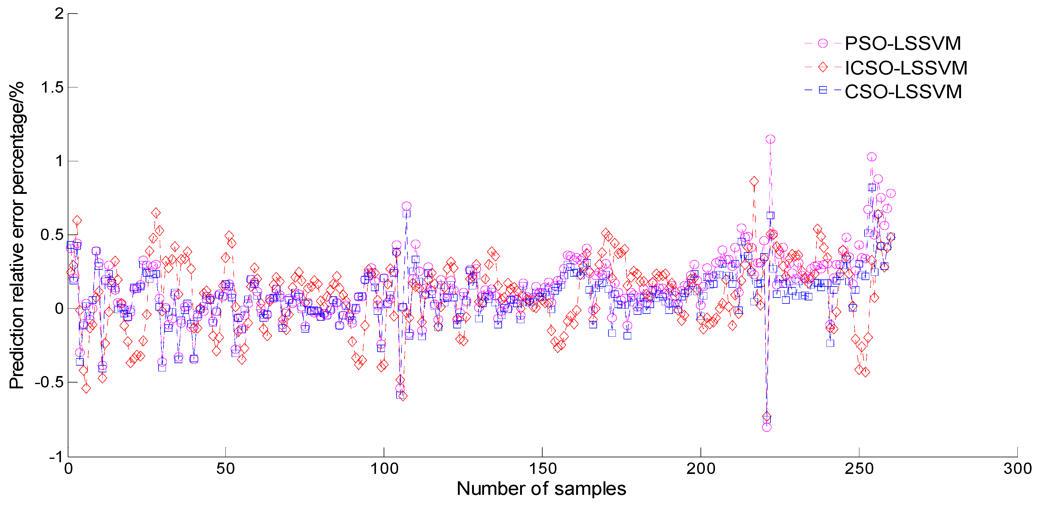
| Model | Maximum Reverse RE/% | Maximum Forward RE/% | Average RE/% |
|---|---|---|---|
| PSO-LSSVM | −0.81 | 1.13 | 0.14 |
| CSO-LSSVM | −0.73 | 0.86 | 0.15 |
| ICSO-LSSM | −0.75 | 0.82 | 0.11 |
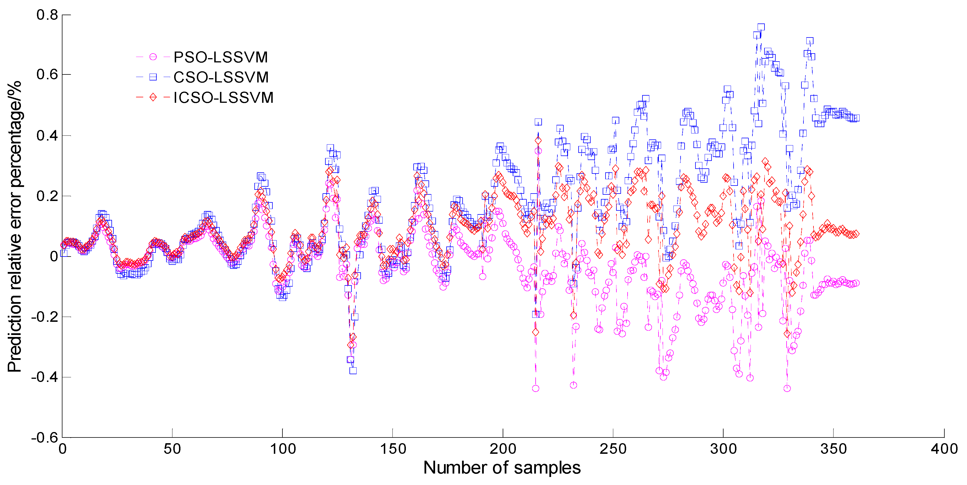
| Model | Maximum Reverse RE/% | Maximum Forward RE/% | Average RE/% |
|---|---|---|---|
| PSO-LSSVM | −0.44 | 0.35 | 0.09 |
| CSO-LSSVM | −0.38 | 0.76 | 0.20 |
| ICSO-LSSVM | −0.29 | 0.38 | 0.11 |
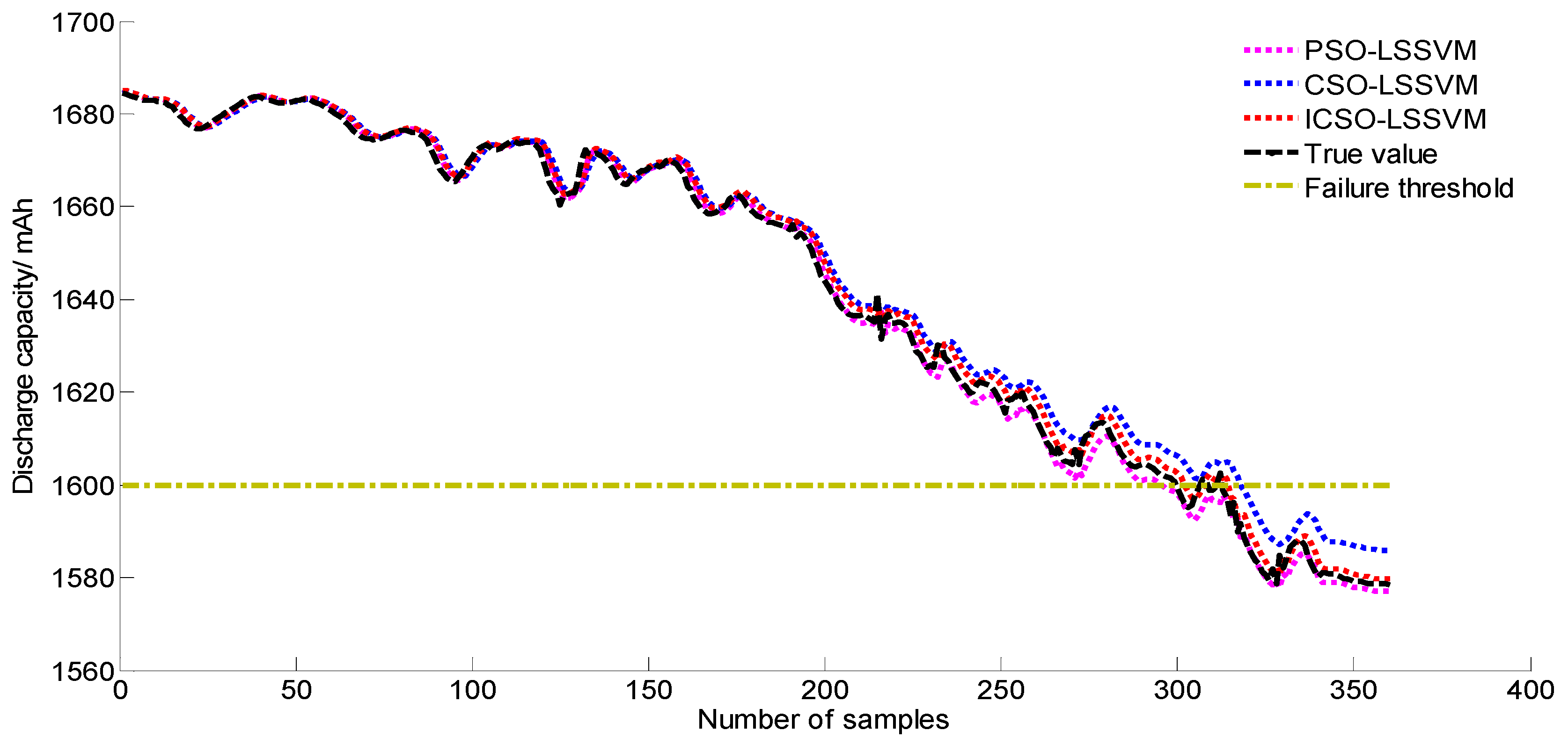
| Battery Type | Prediction Model | True Value of Remaining Life | Predicted Value of Residual Life | |
|---|---|---|---|---|
| NMC1 | PSO-LSSVM | 212 | 220 | 3.77% |
| CSO-LSSVM | 215 | 1.41% | ||
| ICSO-LSSVM | 214 | 0.94% | ||
| NMC2 | PSO-LSSVM | 299 | 295 | 1.33% |
| CSO-LSSVM | 317 | 6.02% | ||
| ICSO-LSSVM | 302 | 1.00% |
© 2019 by the authors. Licensee MDPI, Basel, Switzerland. This article is an open access article distributed under the terms and conditions of the Creative Commons Attribution (CC BY) license (http://creativecommons.org/licenses/by/4.0/).
Share and Cite
Liu, Z.-F.; Li, L.-L.; Tseng, M.-L.; Tan, R.R.; Aviso, K.B. Improving the Reliability of Photovoltaic and Wind Power Storage Systems Using Least Squares Support Vector Machine Optimized by Improved Chicken Swarm Algorithm. Appl. Sci. 2019, 9, 3788. https://doi.org/10.3390/app9183788
Liu Z-F, Li L-L, Tseng M-L, Tan RR, Aviso KB. Improving the Reliability of Photovoltaic and Wind Power Storage Systems Using Least Squares Support Vector Machine Optimized by Improved Chicken Swarm Algorithm. Applied Sciences. 2019; 9(18):3788. https://doi.org/10.3390/app9183788
Chicago/Turabian StyleLiu, Zhi-Feng, Ling-Ling Li, Ming-Lang Tseng, Raymond R. Tan, and Kathleen B. Aviso. 2019. "Improving the Reliability of Photovoltaic and Wind Power Storage Systems Using Least Squares Support Vector Machine Optimized by Improved Chicken Swarm Algorithm" Applied Sciences 9, no. 18: 3788. https://doi.org/10.3390/app9183788