Approximation of Non-Linear Stress–Strain Curve for GFRP Tensile Specimens by Inverse Method


1
Graduate school of Mechanical Engineering, Kongju National University, 1223-24, Cheonan-daero, Seobuk-gu, Cheonan-si, Chungcheongnam-do 31080, Korea
2
Industrial Technology Research Institute, Kongju National University, 1223-24, Cheonan-daero, Seobuk-gu, Cheonan-si, Chungcheongnam-do 31080, Korea
3
Department of Mechanical Engineering (Industrial Technology Research Institute), Kongju National University, 1223-24, Cheonan-daero, Seobuk-gu, Cheonan-si, Chungcheongnam-do 31080, Korea
*
Author to whom correspondence should be addressed.
Appl. Sci. 2019, 9(17), 3474; https://doi.org/10.3390/app9173474
Submission received: 28 July 2019
/
Revised: 16 August 2019
/
Accepted: 18 August 2019
/
Published: 22 August 2019
(This article belongs to the Special Issue Computer Methods for Direct and Inverse Modelling and Simulation)
Abstract
:Studying the characteristics of materials through a finite element analysis (FEA) has various benefits; hence, many studies have been conducted to improve the reliability of the analysis results. In general, the mechanical properties used in FEA for metals and metal composites are stress–strain data obtained through tensile tests, which are used for modeling from a macroscopic perspective. While many studies have been conducted on metal materials, there are limited studies on the analysis of polymer composite materials produced through injection and special processing. In this study, existing inverse methods were applied, and an FEA was conducted to reproduce the axial displacement of the tensile specimens comprising glass fiber-reinforced polymer (GFRP); further, errors were examined by comparing the test and analysis results. To reduce such errors, the experiment and the FEA results were analyzed through parameter optimization based on various empirical formulas. The accuracy of various inverse methods were examined and an inverse method suitable for GFRP was proposed.
1. Introduction
Many studies have been conducted to reduce the weights of automotive [1,2,3,4] and aircraft parts [5,6]. A few of these parts are made of metals; replacing them with polymer plastics satisfies the demand for weight reduction [7,8]. However, polymer plastics exhibit lower strength compared with metal materials [9,10]. To this end, many studies have been conducted to improve the strength of plastics by adding glass or carbon fibers [11,12]. The plastics with such fibers vary the pattern of the stress–strain (S–S) curve, a macroscopic property, and also make it difficult to predict microscopic mechanical properties [13,14]. Unal [15] proposed a method for estimating the S–S curve of a specific or composite material with a large fluctuation in material properties during processing, through fuzzy theory. As there is a considerable difference between the S–S curve derived through fuzzy theory and the behavior of an actual specimen, it is difficult to use the derived S–S curve as the material property for a finite element analysis (FEA).
Recently, studies on models for estimating the S–S curve using the response surface method of design of experiment (DOE), which are referred to as inverse methods, have been conducted [16,17,18]. For inverse methods, basic theories are provided by the American Society for Testing and Materials (ASTM) standards; further, studies to improve the accuracy of property data through mathematical modeling that uses power and exponential functions have been proposed [12,13,14,15,16,17,18,19,20,21,22]. However, as mathematical models may vary depending on the materials, inverse methods have been mostly applied to metals and alloy models. Therefore, it is necessary to select and optimize inverse methods to secure the macroscopic properties of composite materials.
In this study, a method for estimating the macroscopic properties of glass fiber-reinforced polymer (GFRP) tensile specimens, which are commonly used as the lightweight materials of automotive parts, using an inverse method through the finite element method (FEM) was proposed. GFRP specimens were fabricated, and their mechanical properties for tensile deformation were analyzed through tests. Based on the results, various inverse methods were applied for modeling, and the analysis and experiment results were compared. Moreover, parameter optimization was conducted using DOE to select an inverse method most suitable for GFRP among various models. In this process, the maximum number of iterations for optimization was limited to the same value. Moreover, whether the actual properties of GFRP could be estimated was verified through advanced inverse methods—by combining the function with the lowest error.
2. Experiment and FEA Setup
2.1. Experimental Setup (ASTM D638-14)
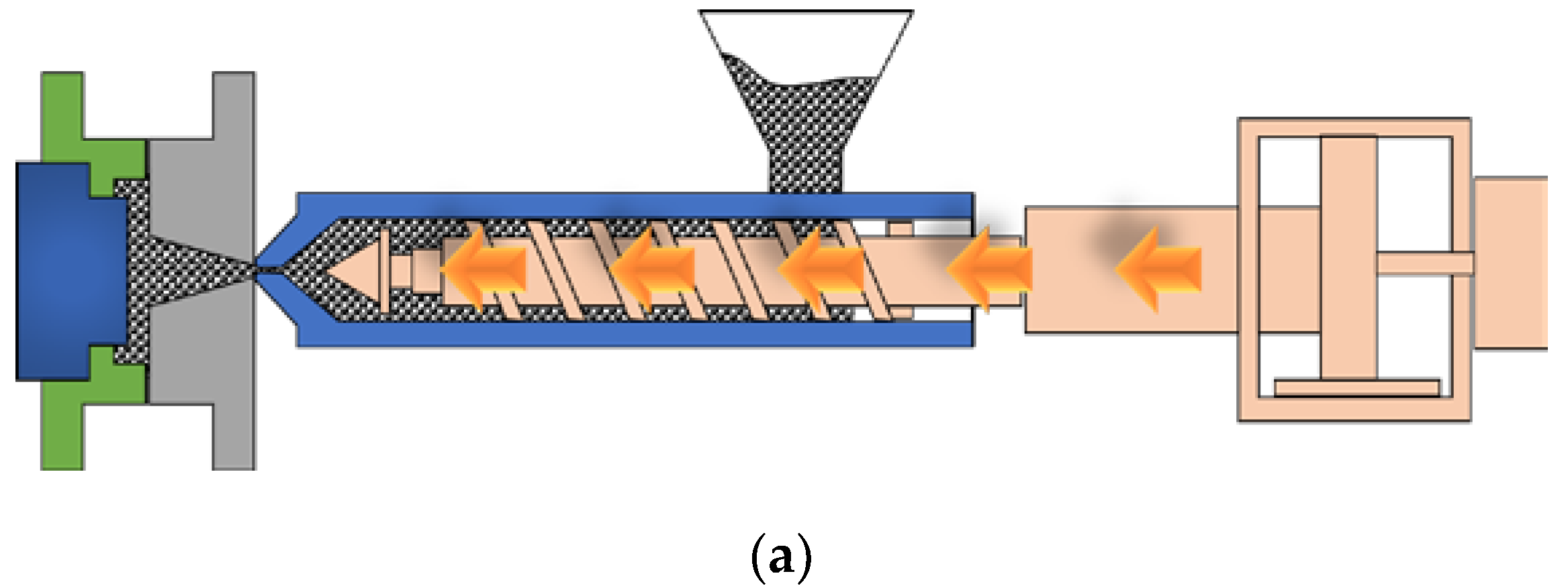
In this experiment, SUPRAN® PP 1320 (wt 20% GF), 1330 (wt 30% GF), and 1340 (wt 40% GF) of SAMBARK LFT were used. Each material is based on polypropylene, and 6~25 mm-long glass fiber accounts for 20%, 30%, and 40% of the total weight of the material. Figure 1a shows the conceptual diagram of the injection process, and Figure 1b shows the test specimen produced by the injection process. The process conditions were set to the injection temperature of 220 °C, pressure of 50 MPa, mold temperature of 4 °C, and cooling time of 15 s, respectively. ASTM D638-14 [23] was applied for the tensile test method. The specimens’ geometry was the dog-bone type, as shown in Figure 1c, and they were fabricated by injection molding, as shown in Figure 1b. To observe the various tendencies of the inverse analysis for GFRP, specimens were fabricated using the properties of GFRP wt 20%, 30%, and 40% GF. Three tensile specimens were fabricated for each GFRP property.
Tensile tests on the specimens were conducted using the MTS 810 material test system. Figure 2 shows the schematic of the tensile test setup. MTS 634 12F was used as the strain gauge equipment for measuring gauge length (), as shown in Figure 1c. Tensile tests were conducted considering a cross-head speed of 5 mm/min, in accordance with ASTM D638-14. The variations of the load and gauge length were obtained as data and reflected to the engineering stress and strain.
Figure 3 shows the properties obtained through tensile tests. For each property, three tests were conducted, and the data corresponding to the median values were selected as representative values. Force () derived from the tensile tester and displacement () derived from the strain gauge were used to express the engineering strain–stress data as and as shown below, along with the true stress presented by ASTM D638-14:
Table 1 lists the Young’s modulus (), Poisson’s ratio (), yield stress (), and tensile strength () derived through tensile tests.
2.2. Finite Element Analysis Setup
Figure 4a–e shows the finite element models of the tensile specimen. In the models, the width (, ) of the tensile specimen was divided into two, four, six, eight, and ten elements, while the aspect ratio of the elements ranged from 0.5 to 1.5. As the geometry of the specimen was not complex, two-dimensional (2D) triangle elements and three-dimensional (3D) tetra elements were not considered.
As for the material properties used for the conformity evaluation of the elements, the experimental parameter () of GFRP wt 20% is commonly applied. The finite element models were analyzed under the conditions shown in Figure 4f based on ASTM D638-14. The left section of the specimen model was set as a fixed section, while the right section was moved at a speed of 5 mm/min. When the FEA was conducted, the reactive force was obtained from the left node set of the specimen model, and the displacement of the gauge length was obtained using the specimen information.
The implicit solver and explicit solver of LS-Dyna R910 were used as FEA tools. The analysis results are shown in Figure 5 according to the division of elements, solver type, and dimensions. Figure 5a shows that the division of elements and solver type did not significantly affect the accuracy of the analysis. However, they significantly affected the analysis time, as shown in Figure 5b.
In general, models with implicit solvers, 3D elements, and a large number of divisions are selected to improve the accuracy of the analysis results. However, when estimating the mechanical properties, it was confirmed that selecting a model with explicit solvers, 2D elements, and a small number of divisions did not result in large differences. Therefore, in this study, models with explicit solvers, 2D elements, and a small number of divisions were used to reduce the analysis time.
2.3. Inverse Methods
Inverse methods are useful when the change in the thickness of the necking zone cannot be accurately measured after the yield stress is reached. They can be used as correction measures for the stress value when the engineering S–S curve obtained experimentally is different from the engineering S–S curve obtained using the FEA.
Inverse methods to obtain the true stress are largely divided into power law models and exponential law models. The models of Hollomon [24], Ludwik [25], Swift [26], and Gosh [27] shown in Equations (4)–(7) can be considered as representative power law models. The models of Voce [28] and Hockett–Sherby [29] shown in Equations (8) and (9) can be considered as representative exponential law models. In each model, c is a material parameter, and its initial value is determined using the logarithmic curve method given in ASTM E646-16 [30].
In this theoretical model, parameters of the test environments such as the ambient temperature and test speed can be included. However, in this study, the parameters of the test environments were not considered, as the aim of the study was to propose an inverse method that could approximate the plastic deformation behavior of GFRP.
Figure 6 shows the true S–S curves derived using Equations (4)–(9). In the figure, test data for the curves were included for a comparison between the true stress and the engineering stress.
It was found that the true S–S data obtained using the ASTM D638-14, Hollomon, Ludwik, and Swift equations were not significantly different from the experimental data. In contrast, the Gosh model and the exponential law model exhibited significant differences from the experimental data. The physically reliable and accurate data of the engineering S–S curve and all true stress curves were estimated values.
The true S–S curve data were used as the mechanical properties of the FEA software, and were entered as the point data of 100 divisions based on the total strain. The engineering S–S curve data shown in Figure 7 were derived using the simulation shown in Figure 4f.
To quantitatively demonstrate the expression accuracy of the analysis results for an actual physical phenomenon, the engineering S–S curve obtained experimentally was compared with the engineering S–S curve obtained from the analysis, as shown in Equation (10). Through this process, an inverse analysis model that could accurately express actual physical phenomena was found.
The difference in the engineering S–S curves obtained using the experimental and analysis data was expressed as , as shown in Equation (10), and the average of the absolute values of such data was expressed as , as shown in Equation (11). The average of the errors generated from all of the properties for each inverse method was expressed as , as shown in Equation (12).
Figure 7 shows the results of the FEA that was conducted using the estimation equations. For the engineering S–S curves, the experimental data were significantly different from the analysis data, and the c value of ASTM E646-16 resulted in inaccurate results. This can also be observed in Figure 8, which shows the graphs obtained using Equation (10) for a comparison. The arithmetic average values for are listed in Table 2. Among the power law models, the Gosh model exhibited the most accurate approximations of the deformation when compared to the actual values, and among the exponential law models, the Voce model exhibited the best approximation.
3. Optimization of Inverse Methods
To approximate the experiment and analysis results for the engineering S–S curve, the value of the material parameter (c) of the inverse method must be adjusted. To this end, optimization was performed using the minimum error between the experimental and the analysis results as the objective function.
The optimization formulation process is shown in Equations (13)–(18). To improve the accuracy of the engineering S–S curve obtained using the FEA, an objective function that minimizes was constructed, and the material parameter was adjusted in the 30% range from the initial value used given in ASTM E646-16.
Find:
Minimize:
Subject to:
Parameter Optimization
D-optimal DOE was applied to minimize the number of iterations in the optimization process [31]. Here, the process of deriving the error range between the experimental and FEA results and adjusting the parameters was repeated. The same optimization method and number of iterations were applied to all inverse methods. Figure 9 shows the analysis results. As the engineering stress and true stress models based on ASTM D638-14 were excluded from the optimization targets, the errors indicated by Figure 7 could be observed. When the optimized inverse methods were used in the FEA, the results were very similar to the engineering S–S curve obtained from the experiment. The error of the optimized inverse method () can be seen in Figure 10. The error patterns of the power law and that of the exponential law models were reversed, and it can be seen that the Hockett–Sherby formula was very accurately optimized.
The average of cumulative errors () is listed in Table 3. Considerable errors were observed in the three data points excluded from the optimization process. Among the power law models, the Swift model obtained the most accurate results, followed by the Ludwik, Gosh, and Hollomon models. Among the exponential law models, the Voce model obtained the most accurate results, followed by the Hockett–Sherby model.
4. Results of Advanced Inverse Method
4.1. Advanced Inverse Method
It is known that power law models are suitable for metals with the BCC structure, such as steel, and that exponential law models are suitable for metals with the FCC structure, such as aluminum and copper. In addition, Kim–Tuan [32] combined the power law (Swift) model and the exponential law (Voce) model for the efficient management of various metal properties, as shown in the following equations. They proposed advanced inverse methods to adjust the proportion of each model using material parameters.
These advanced inverse methods are compatible with various properties, and can correct the errors of the power and the exponential laws. Figure 10 shows that the error () values of the power laws and exponential laws optimized in this study had opposite patterns. Therefore, if the accurately derived power and exponential laws are selected and combined into one equation, better accuracy can be obtained. Through the optimization results, the two models with the lowest average property error () values were selected from the power and exponential laws.
The Swift and Ludwik models from the power laws and the Voce and Hockett–Sherby models from the exponential laws were combined to use the advanced inverse methods of the following equations. In each advanced inverse method, “” is the material parameter that adjusts the proportions of the power and exponential laws.
4.2. Simulation and Optimization
Figure 11 shows the values, including the optimization results of the advanced inverse methods. Items 8–12 in Table 3 are the optimized results of the advanced inverse methods. It can be seen that the advanced inverse methods can estimate the actual behavior of the specimen more accurately. By comparing the optimized , it is seen that the Swift–Voce model exhibited the most approximate estimate of 0.18 MPa. When the levels of factors increased in the DOE, the order of the data analysis also increased; hence, the non-linear response must be considered. Therefore, the number of factors must be reduced to increase the precision and decrease the cost [33]. In many studies, the number of factors was reduced, and the DOE as well as the optimization was performed for the simplified models. In addition, their performances were verified [34]. As the advanced inverse methods have more factors than the normal inverse methods, it is difficult to obtain high accuracy under the same DOE and with the same number of optimization iterations. The Hockett–Sherby model of the exponential law exhibited the most accurate value.
However, the advanced inverse models exhibited higher accuracy compared with the inverse models, even though they had two to three times more factors (Figure 11). This indicates that plastic and composite materials are significantly different from metals, which can be expressed by one power or exponential function.
5. Conclusions
In this study, the experiment results were compared with the results of the analysis, which was conducted by applying the proposed empirical equations to examine the S–S curve of GFRP tensile specimens through a FEA. In the study, inverse models were defined using the coefficients based on ASTM E646-16, and the results of the FEA were found to be significantly different from the experiment values. Among the models by the logarithmic curve, the Voce model exhibited the smallest difference of less than . To improve the accuracy of the analysis results, the factors of the inverse methods were optimized, and curve fitting was performed. As a result, a relatively low error rate was observed, compared with the existing models. After optimization, the Hockett–Sherby model exhibited the lowest error rate. These results indicate that the application of the Hockett–Sherby model can improve the accuracy of the analysis results when a FEM analysis is conducted using the macroscopic mechanical properties of GFRP.
Author Contributions
D.S.S., Y.S.K. and E.S.J. conceived and designed the experiments; D.S.S., Y.S.K. and E.S.J. performed the experiments; D.S.S., Y.S.K. and E.S.J. analyzed the data; D.S.S., Y.S.K. and E.S.J. contributed reagents/materials/analysis tools; D.S.S., Y.S.K. and E.S.J. wrote the paper.
Funding
This research was financially supported by The Ministry of Trade Industry and Energy (MOTIE), “A project for overcome the crisis of vehicle pars (P0005816)”.
Conflicts of Interest
The authors declare no conflict of interest.
Nomenclature
| Center width of tensile specimen | |
| Total width of tensile specimen | |
| Thickness of tensile specimen | |
| Length of tensile specimen | |
| Total length of tensile specimen | |
| Gauge length = Original distance between gage marks | |
| Increment of distance between gage marks | |
| Displacement in FEA | |
| Radius | |
| Reactive force | |
| Engineering stress in experiment of ASTM D638-14 | |
| Engineering strain in experiment of ASTM D638-14 | |
| True stress in experiment of ASTM D638-14 | |
| Engineering stress in FEA | |
| Engineering strain in FEA | |
| Maximum number of data points that express stress–strain | |
| Order of data that express stress-strain, | |
| Sequential stress values of the stress–strain curve derived from FEA | |
| Sequential stress values of the stress–strain curve derived from an experiment | |
| E | Young’s modulus |
| Poisson’s ratio | |
| Yield stress | |
| Yield strain | |
| Maximum number of material properties | |
| Value that expresses the order of a material property, | |
| Equation number of the inverse method, | |
| Difference in the experiment and analysis for the engineering stress | |
| Average of the differences between the experiment and the analysis | |
| Average of the differences between the experiment and the analysis for the entire material properties | |
| Material parameter of inverse model | |
| Material parameter of advanced model | |
| Maximum number of material parameters by inverse method | |
| Value that expresses the order of a material parameter |
References
- Carlo, B.N.; Andrea, T.; Raaele, C.; Giovanni, B.; Davide, S.P. Assessment of residual elastic properties of a damaged composite plate with combined damage index and finite element methods. Appl. Sci. 2019, 9, 2579. [Google Scholar]
- Mazzon, E.; Habas-Ul, A.; Habas, J.P. Lightweight rigid foams from highly reactive epoxy resins derived from vegetable oil for automotive applications. Eur. Polym. J. 2015, 68, 546–557. [Google Scholar] [CrossRef]
- Hwang, Y.J.; Kang, S.K.; Kim, J.B.; Lee, S.S.; Choi, C.G.; Son, J.H. Topology optimal design for lightweight shape of the vehicle mechanical component. J. Korean Soc. Precis. Eng. 2003, 20, 177–184. [Google Scholar]
- Ishikawa, T.; Amaoka, K.; Masubuchi, Y.; Yamamoto, T.; Yamamoto, A.; Arai, M.; Takahashi, J. Overview of automotive structural composites technology developments in Japan. Compos. Sci. Technol. 2018, 155, 221–246. [Google Scholar] [CrossRef]
- Katunin, A.; Sul, P.; Łasica, A.; Dragan, K.; Krukiewicz, K.; Turczyn, R. Damage resistance of CSA-doped PANI/epoxy CFRP composite during passing the artificial lightning through the aircraft rivet. Eng. Fail. Anal. 2017, 82, 116–122. [Google Scholar] [CrossRef]
- Mouritz, A.P. Advances in understanding the response of fibre-based polymer composites to shock waves and explosive blasts. Compos. Part A Appl. Sci. Manuf. 2019, 125, 105502. [Google Scholar] [CrossRef]
- Talha Junaid, M.; Elbana, A.; Altoubat, S.; Al-Sadoon, Z. Experimental study on the effect of matrix on the flexural behavior of beams reinforced with Glass Fiber Reinforced Polymer (GFRP) bars. Compos. Struct. 2019, 222, 110930. [Google Scholar]
- Yuan, Y.; Niu, K.; Wang, Z. Compressive strength prediction of fibre reinforced polymer composites under lateral disturbance. Polym. Test. 2019, 78, 105952. [Google Scholar] [CrossRef]
- Henning, F.; Kärger, L.; Dörr, D.; Schirmaier, F.J.; Seuffert, J.; Bernath, A. Fast processing and continuous simulation of automotive structural composite components. Compos. Sci. Technol. 2019, 171, 261–279. [Google Scholar] [CrossRef]
- Stewart, R. Lightweighting the automotive market. Reinf. Plast. 2009, 53, 14–16. [Google Scholar] [CrossRef]
- Hwang, Y.K.; Eun, I.U.; Lee, C.M.; Seo, Y.W. Development of Lightweight Moving Table for Linear Motor using Composite Materials. J. Korean Soc. Precis. Eng. 2010, 27, 7–13. [Google Scholar]
- You, H.Y.; Park, S.H. Warpage analysis of a door carrier plate in the injection molding considering the characteristics of LFT. J. Korea Acad. Ind. Coop. Soc. 2013, 14, 3625–3630. [Google Scholar]
- Seon, G.; Makeev, A.; Schaefer, J.D.; Justusson, B. Measurement of interlaminar tensile strength and elastic properties of composites using open-hole compression testing and digital image correlation. Appl. Sci. 2019, 9, 2647. [Google Scholar] [CrossRef]
- Hohe, J.; Beckmann, C.; Paul, H. Modeling of uncertainties in long fiber reinforced thermoplastics. Mater. Des. 2015, 66, 390–399. [Google Scholar] [CrossRef]
- Ünal, O.; Demir, F.; Uygunoglua, T. Fuzzy logic approach to predict stress–strain curves of steel fiber-reinforced concretes in compression. Build. Environ. 2007, 42, 3589–3595. [Google Scholar] [CrossRef]
- Zhao, K.; Wang, L.; Chang, Y.; Yan, J. Identification of post-necking stress–strain curve for sheet metals by inverse method. Mech. Mater. 2016, 92, 107–118. [Google Scholar] [CrossRef]
- Flayeh, A.H.; Toopchi-Nezhad, H.; TahamouliRoudsari, M. The use of fiberglass textile-reinforced mortar (TRM) jacketing system to enhance the load capacity and confinement of concrete columns. In Proceedings of the 2018 2nd International Conference for Engineering Technology and Sciences of Al-Kitab (ICETS), Karkuk, Iraq, 4–6 December 2018; pp. 66–71. [Google Scholar]
- Zhang, Z.L.; Hauge, M.; Odegard, J.; Thaulow, C. Determining material true stress-strain curve from tensile specimens with rectangular cross-section. Int. J. Solids Struct. 1999, 36, 3497–3516. [Google Scholar] [CrossRef]
- Kim, J.H.; Serpantie, A.; Barlat, F.; Pierron, F.; Lee, M.G. Characterization of the post-necking strain hardening behavior using the virtual fields method. Int. J. Solids Struct. 2013, 50, 3829–3842. [Google Scholar] [CrossRef] [Green Version]
- Joun, M.S.; Eom, J.G.; Lee, M.C. A new method for acquiring true stress–strain curves over a large range of strains using a tensile test and finite element method. Mech. Mater. 2008, 40, 586–593. [Google Scholar] [CrossRef]
- Kamaya, M.; Kawakubo, M. A procedure for determining the true stress–strain curve over a large range of strains using digital image correlation and finite element analysis. Mech. Mater. 2011, 43, 243–253. [Google Scholar] [CrossRef]
- Dziallach, S.; Bleck, W.; Blumbach, M.; Hallfeldt, T. Sheet metal testing and flow curve determination under multiaxial conditions. Adv. Eng. Mater. 2007, 9, 987–994. [Google Scholar] [CrossRef]
- ASTM. Standard Test Method for Tensile Properties of Plastics; ASTM D638-14; ASTM: West Conshohocken, PA, USA, 2014. [Google Scholar]
- Hollomon, J.H. Tensile deformations. Trans. Metall. Soc. AIME 1945, 162, 268–290. [Google Scholar]
- Ludwik, P. Elemente der Technologischen Mechanik; Springer: Berlin, Germany, 1909. [Google Scholar]
- Swift, H.W. Plastic instability under plane stress. J. Mech. Phys. Solids 1952, 1, 1–18. [Google Scholar] [CrossRef]
- Gosh, A.K. Tensile instability and necking in materials with strain hardening and strain-rate hardening. Acta Metall. 1977, 25, 1413–1424. [Google Scholar] [CrossRef]
- Voce, E. The relationship between stress and strain for homogeneous deformation. J. Inst. Met. 1948, 74, 537–562. [Google Scholar]
- Hockett, J.E.; Sherby, O.D. Large strain deformation of polycrystalline metals at low homologous temperatures. J. Mech. Phys. Solids 1975, 23, 87–98. [Google Scholar] [CrossRef]
- ASTM. Tensile Strain-Hardening Exponents (N-Values) of Metallic Sheet Materials; ASTM E646-16; ASTM: West Conshohocken, PA, USA, 2016. [Google Scholar]
- Cook, R.D.; Nachtsheim, C.J. A comparison of algorithms for constructing exact D-optimal designs. Technometrics 1980, 22, 315–324. [Google Scholar] [CrossRef]
- Kim, Y.S.; Pham, Q.T.; Kim, C.I. New stress-strain model for identifying plastic deformation behavior of sheet materials. J. Korean Soc. Precis. Eng. 2017, 34, 273–279. [Google Scholar] [CrossRef]
- Lee, D.W.; Cho, S.S. Tension estimation of tire using neural networks and DOE. J. Korean Soc. Precis. Eng. 2011, 28, 814–820. [Google Scholar]
- Doh, J.H.; Lee, J.S. Approximate multi-objective optimization of a wall-mounted monitor bracket arm considering strength design conditions. Trans. Korean Soc. Mech. Eng. A 2015, 39, 535–541. [Google Scholar] [CrossRef]
Figure 1.
ASTM D638-14 specimen for tensile test: (a) schematic diagram of injection molding; (b) test specimen of glass fiber-reinforced polymer (GFRP); (c) specification of specimen for ASTM D638-14.
Figure 1.
ASTM D638-14 specimen for tensile test: (a) schematic diagram of injection molding; (b) test specimen of glass fiber-reinforced polymer (GFRP); (c) specification of specimen for ASTM D638-14.

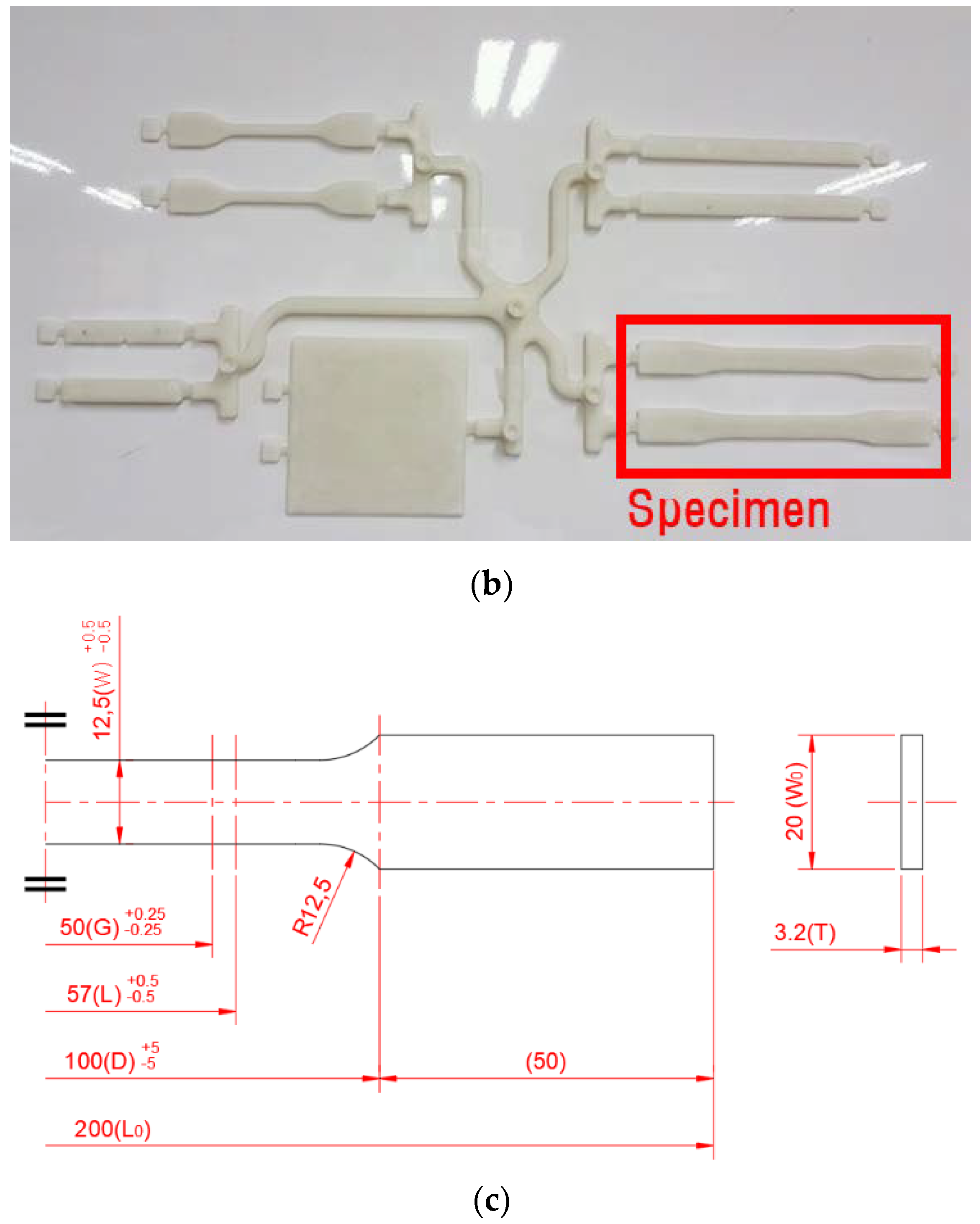
Figure 2.
Schematic of tensile test.
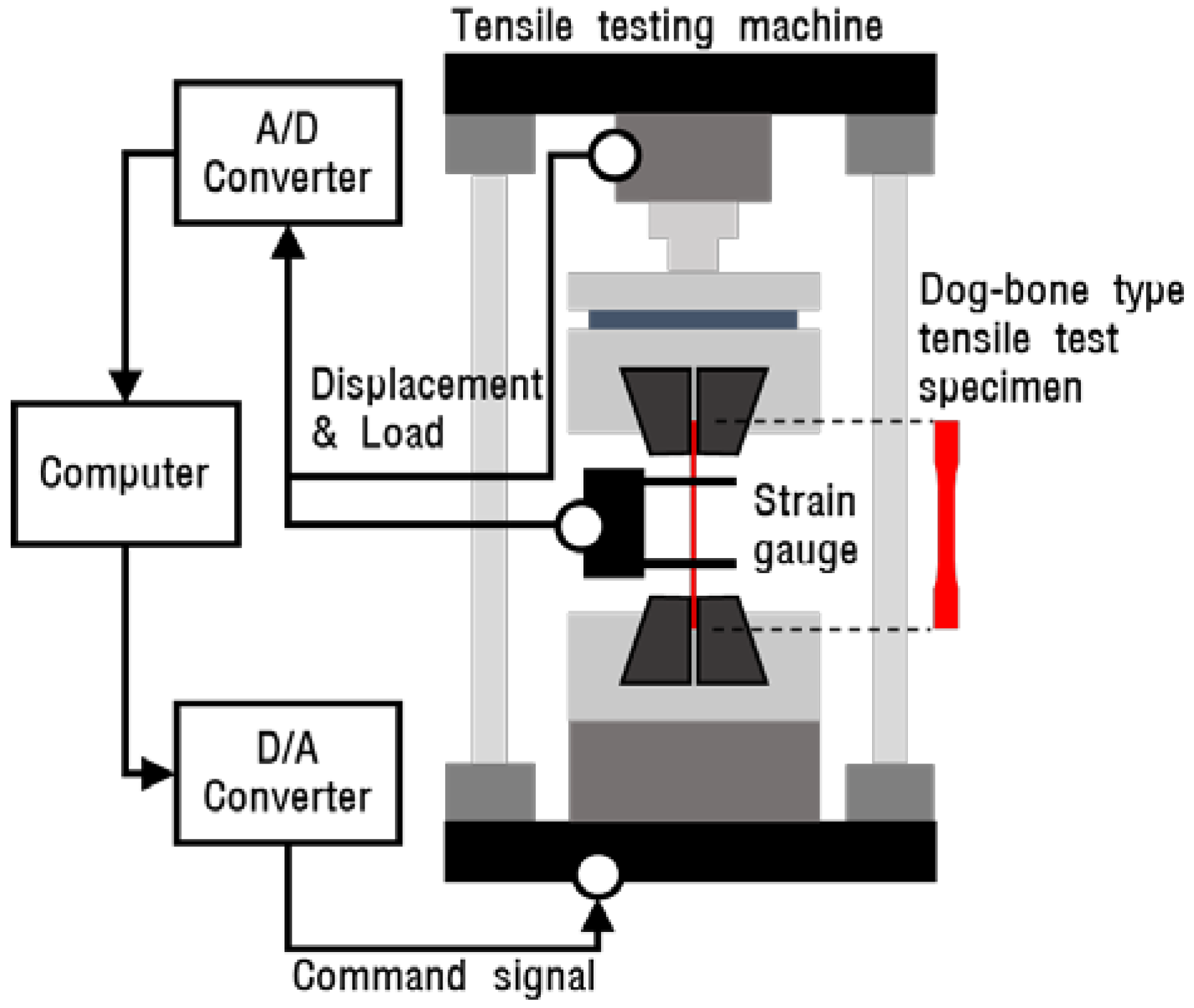
Figure 3.
Results of the tensile test: (a) engineering strain–stress curve of experimental; (b) offset yield stress of GFRP.
Figure 3.
Results of the tensile test: (a) engineering strain–stress curve of experimental; (b) offset yield stress of GFRP.
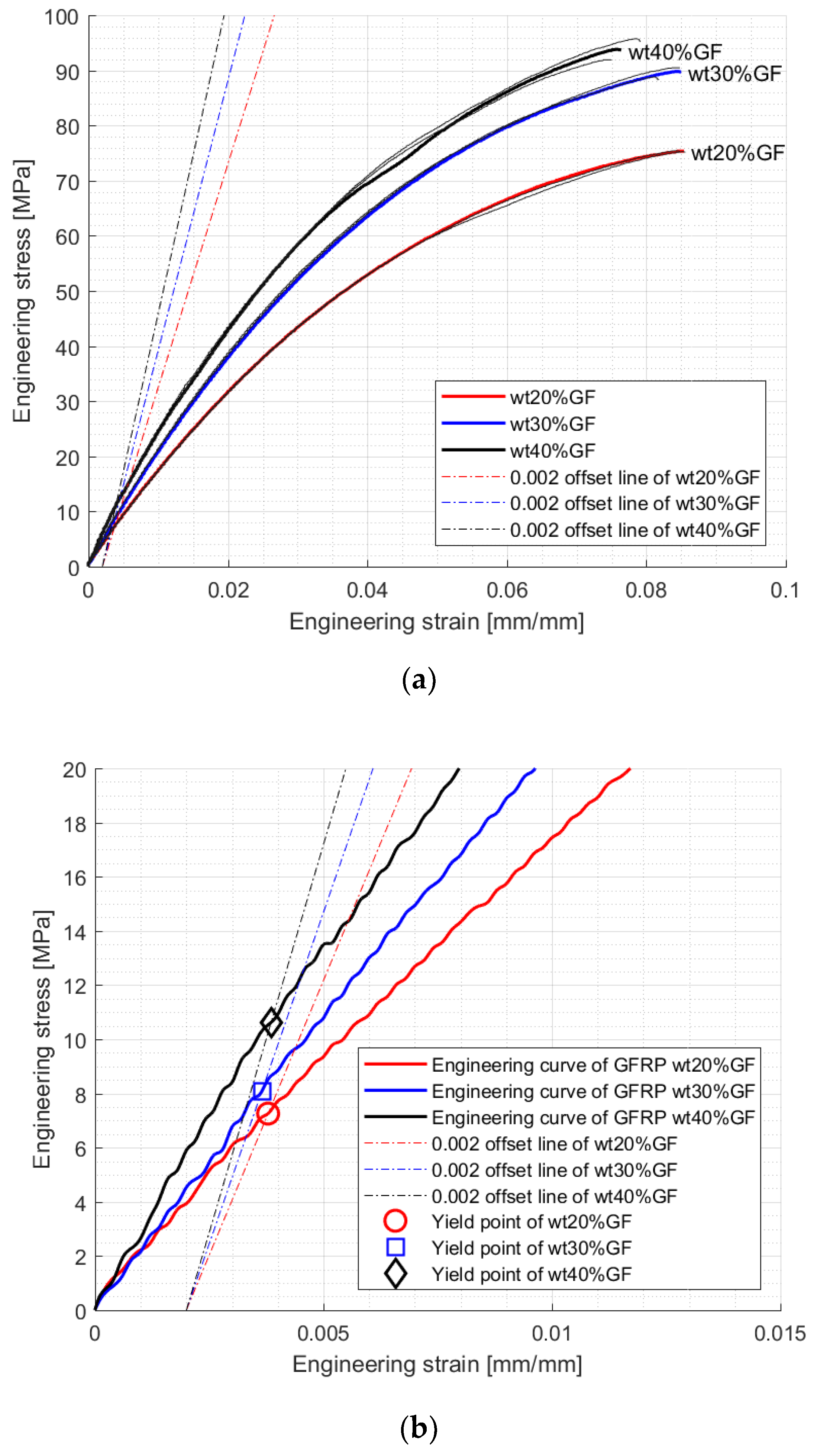
Figure 4.
Finite element models for tensile test specimens: (a) element division 2 (average element size: 8.125 mm); (b) element division 4 (average element size: 4.0625 mm); (c) element division 6 (average element size: 2.7083 mm); (d) element division 8 (average element size: 2.0313 mm); (e) element division 10 (average element size: 1.625 mm); (f) finite element analysis model for tensile specimen.
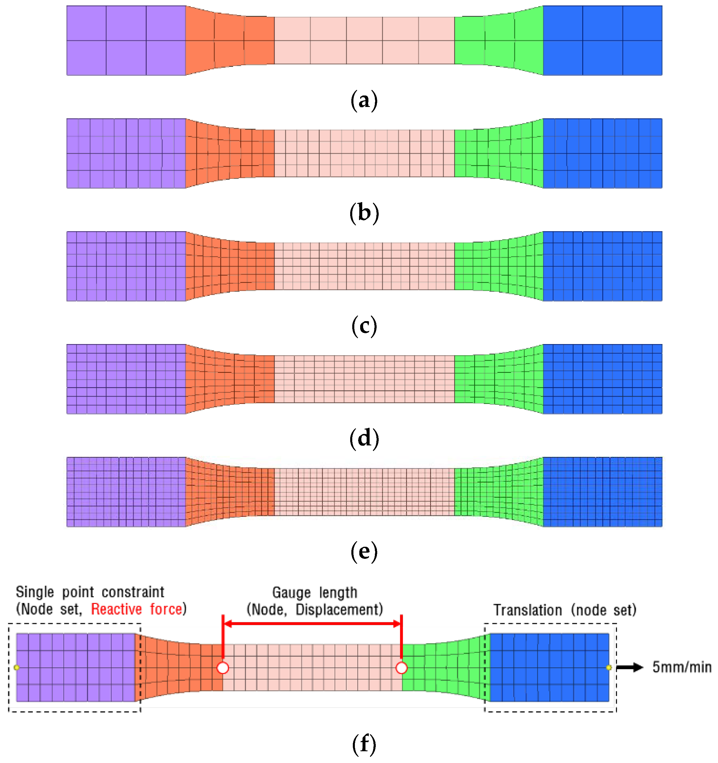
Figure 5.
Results of the finite element analysis: (a) result of the finite element analysis; (b) total CPU time by element type and solver type.
Figure 5.
Results of the finite element analysis: (a) result of the finite element analysis; (b) total CPU time by element type and solver type.
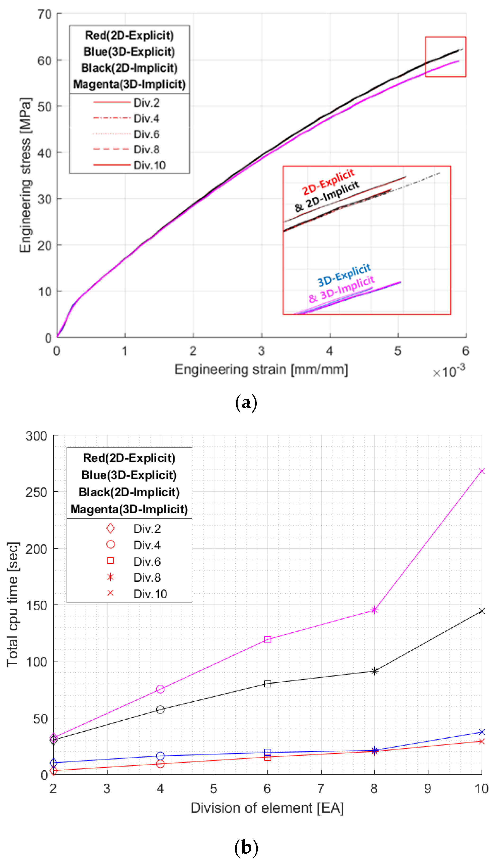
Figure 6.
Theoretical true S–S curves: (a) GFRP wt 20% GF; (b) GFRP wt 30% GF; (c) GFRP wt 40% GF.
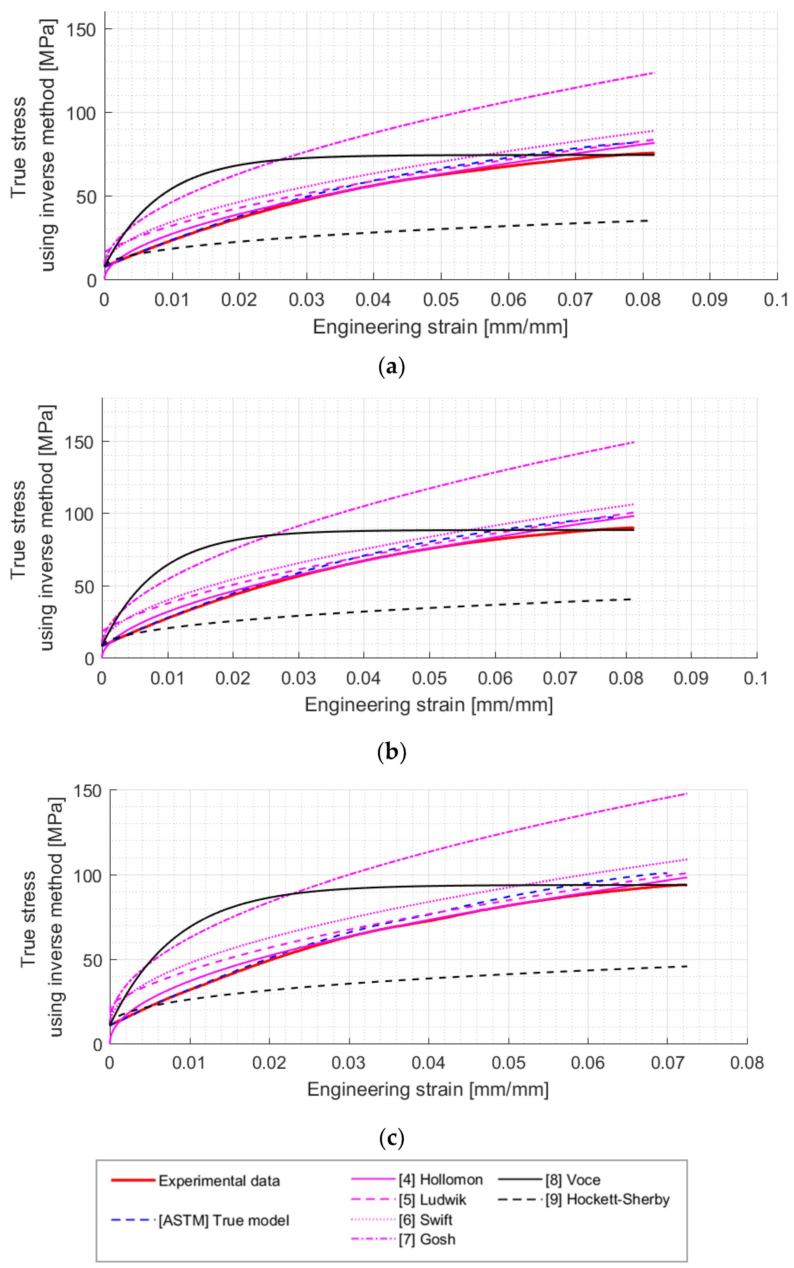
Figure 7.
Experimental curves and finite element analysis (FEA) results: (a) inverse models of GFRP wt 20% GF; (b) inverse models of GFRP wt 30% GF; (c) inverse models of GFRP wt 40% GF.
Figure 7.
Experimental curves and finite element analysis (FEA) results: (a) inverse models of GFRP wt 20% GF; (b) inverse models of GFRP wt 30% GF; (c) inverse models of GFRP wt 40% GF.

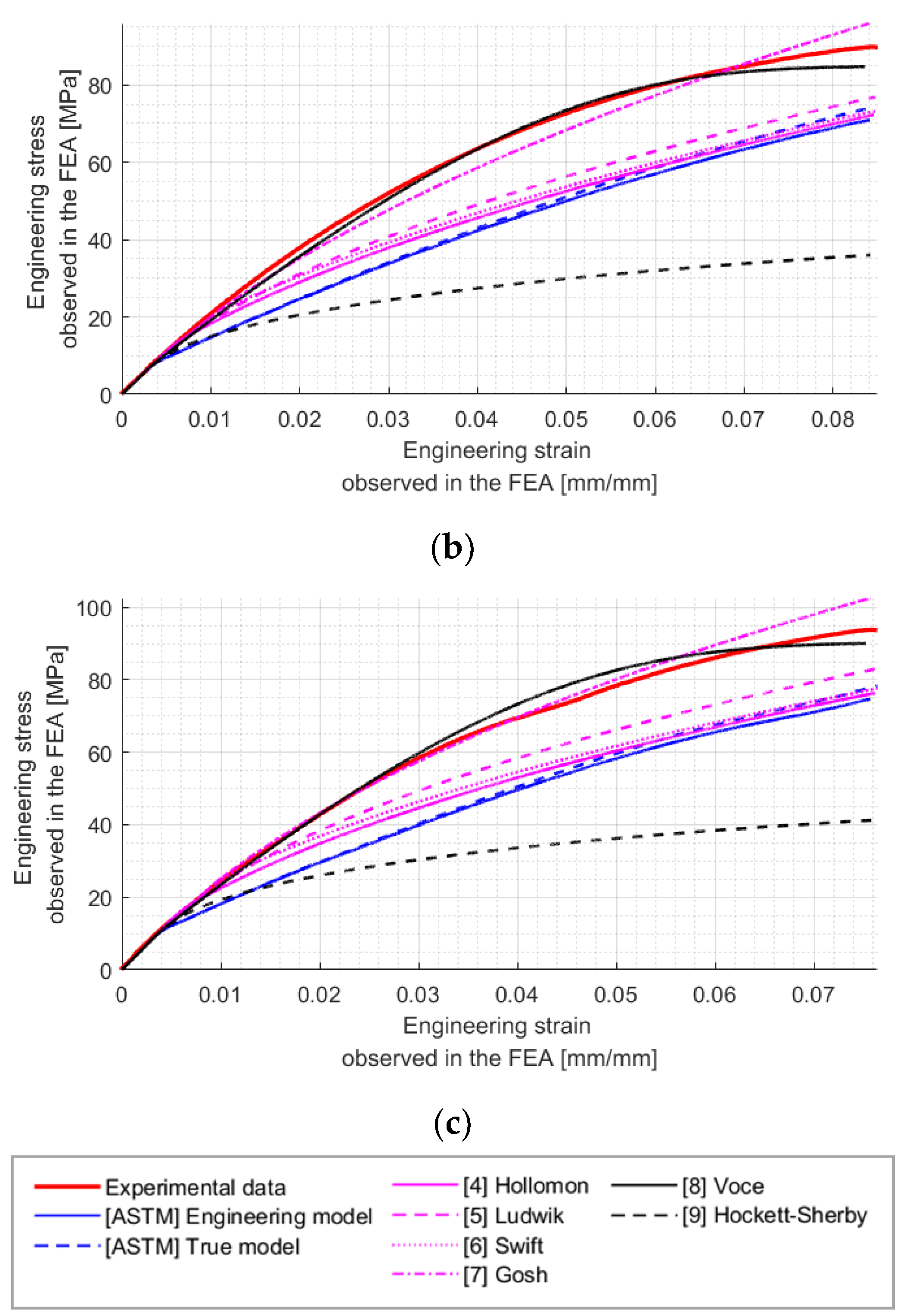
Figure 8.
Differences between inverse models and experimental results: (a) inverse models of GFRP wt 20% GF; (b) inverse models of GFRP wt 30% GF; (c) inverse models of GFRP wt 40% GF.
Figure 8.
Differences between inverse models and experimental results: (a) inverse models of GFRP wt 20% GF; (b) inverse models of GFRP wt 30% GF; (c) inverse models of GFRP wt 40% GF.
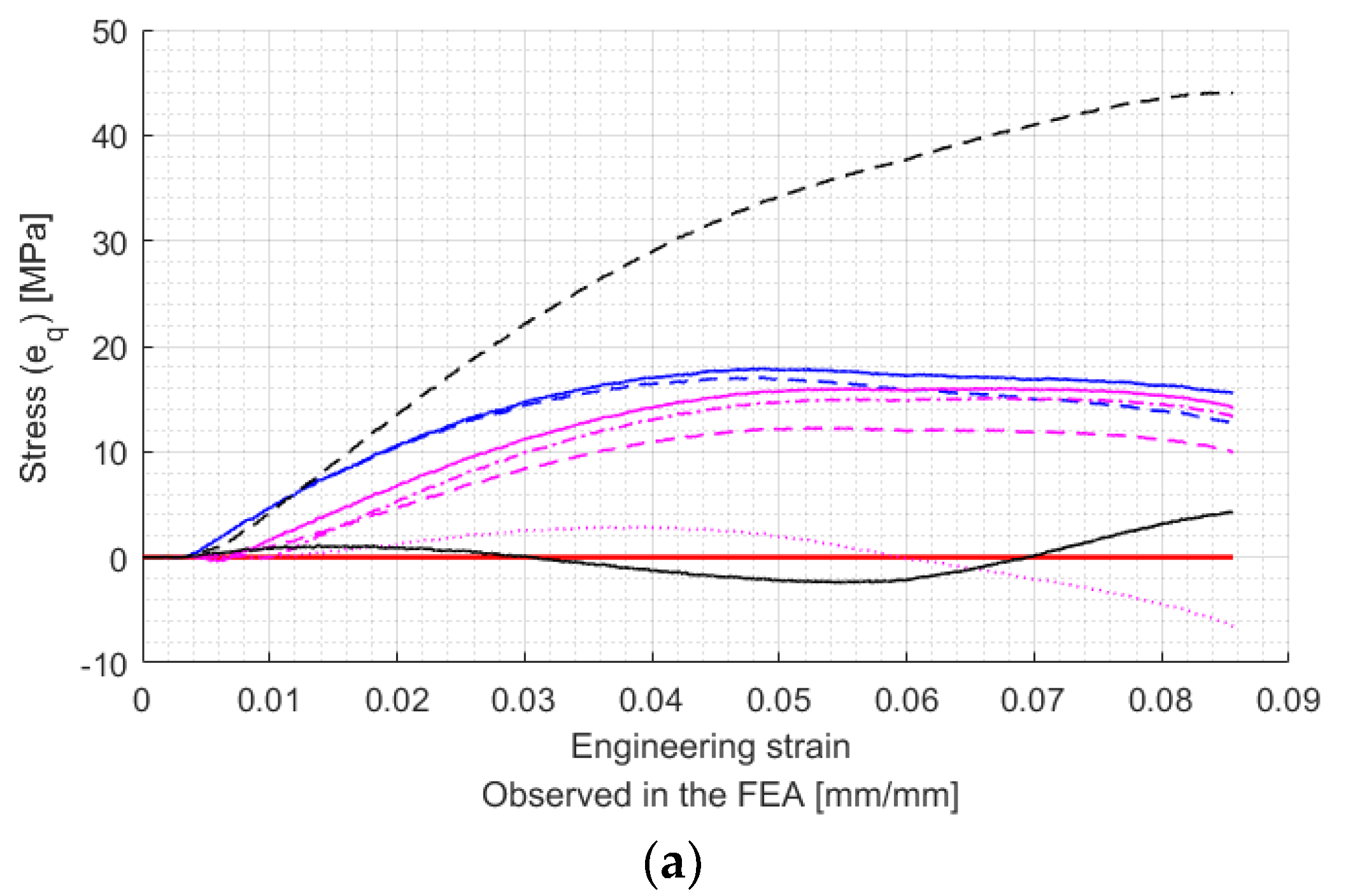
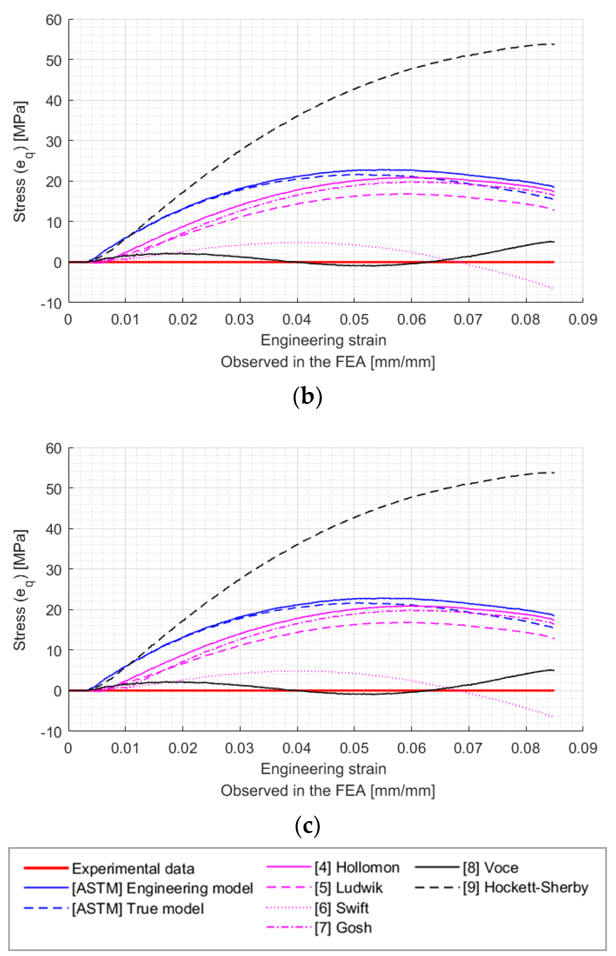
Figure 9.
Engineering S–S curve of the optimized models: (a) inverse models of GFRP wt 20%GF; (b) inverse models of GFRP wt 30% GF; (c) inverse models of GFRP wt 40% GF.
Figure 9.
Engineering S–S curve of the optimized models: (a) inverse models of GFRP wt 20%GF; (b) inverse models of GFRP wt 30% GF; (c) inverse models of GFRP wt 40% GF.

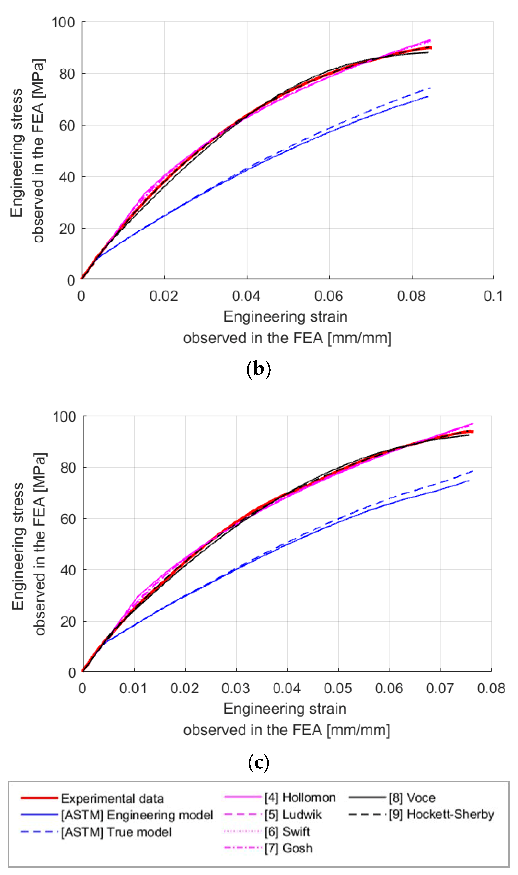
Figure 10.
Error values of the optimized inverse method models: (a) optimized inverse models of GFRP wt 20% GF; (b) optimized inverse models of GFRP wt 30% GF; (c) optimized inverse models of GFRP wt 40% GF.
Figure 10.
Error values of the optimized inverse method models: (a) optimized inverse models of GFRP wt 20% GF; (b) optimized inverse models of GFRP wt 30% GF; (c) optimized inverse models of GFRP wt 40% GF.
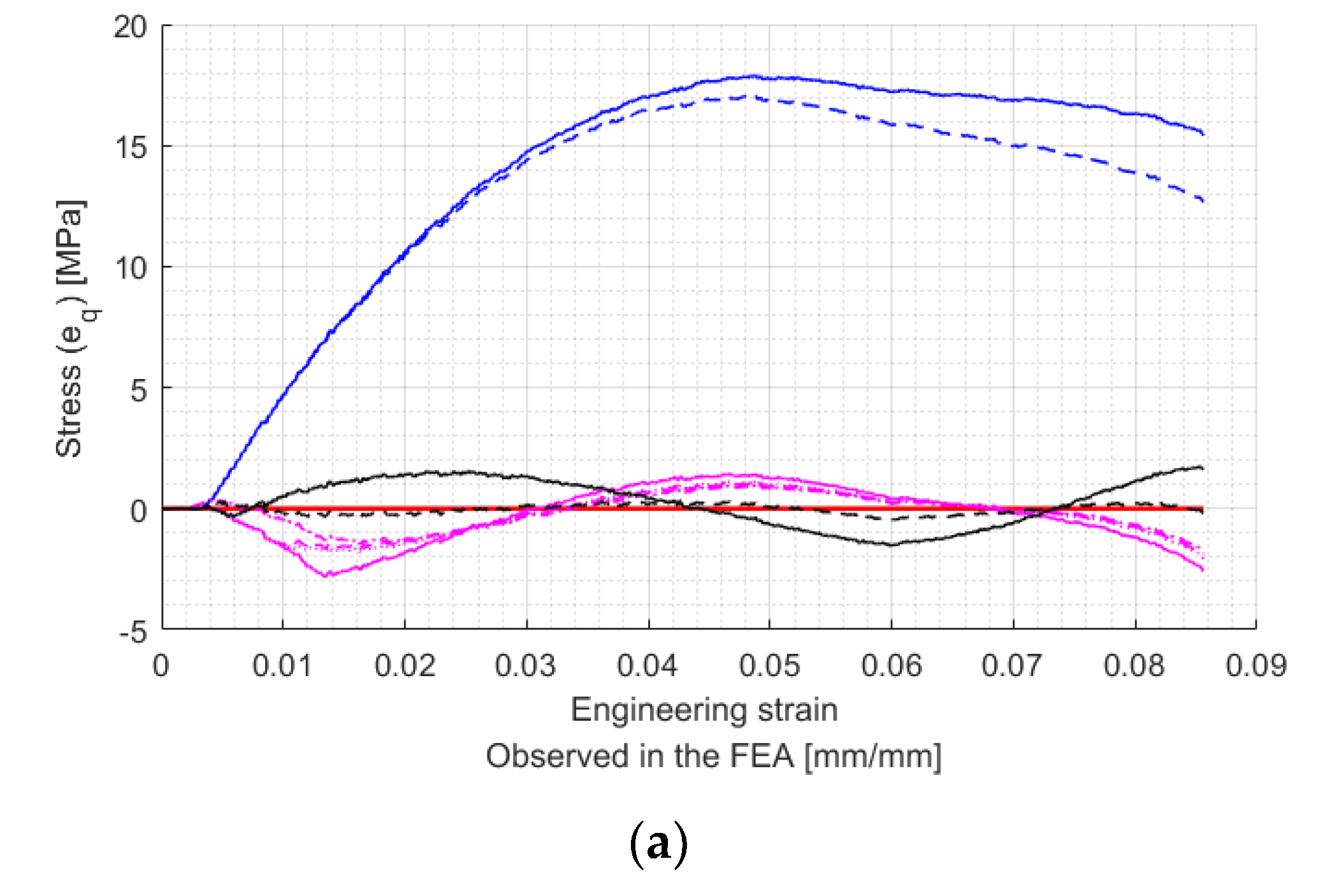

Figure 11.
Error values of the optimized inverse method.


Table 1.
Mechanical properties of GFRP.
| Symbols | Units | wt 20% GF | wt 30% GF | wt 40% GF |
|---|---|---|---|---|
| MPa | 4082.40 | 4833.49 | 5717.59 | |
| - | 0.35 | 0.38 | 0.4 | |
| MPa | 7.25 | 8.08 | 10.62 | |
| - | 0.0038 | 0.0037 | 0.0039 | |
| 1.05 | 1.11 | 1.21 | ||
| MPa | 75.33 | 89.72 | 93.83 |
Table 2.
Errors between experimental results and FEA results.
| No. | Eq. | Applied S–S Curve Model | ||||
|---|---|---|---|---|---|---|
| wt 20% GF | wt 30% GF | wt 40% GF | ||||
| 1 | 1 | ASTM Engineering model | 13.54 | 17.00 | 15.75 | 15.43 |
| 2 | 3 | ASTM True model | 12.62 | 15.97 | 14.67 | 14.42 |
| 3 | 4 | Hollomon | 11.37 | 14.41 | 12.77 | 12.85 |
| 4 | 5 | Ludwik | 8.50 | 11.43 | 8.29 | 9.41 |
| 5 | 6 | Swift | 10.33 | 13.28 | 11.38 | 11.66 |
| 6 | 7 | Gosh | 1.87 | 2.85 | 2.06 | 2.26 |
| 7 | 8 | Voce | 1.32 | 1.39 | 1.91 | 1.54 |
| 8 | 9 | Hockett–Sherby | 26.59 | 33.03 | 30.51 | 30.05 |
Table 3.
Optimized values of the advanced inverse method.
| No. | Eq. | Applied S-S Curve Model | ||||
|---|---|---|---|---|---|---|
| wt 20% GF | wt 30% GF | wt 40% GF | ||||
| 1 | 1 | ASTM Engineering model | 13.54 | 17.00 | 15.75 | 15.43 |
| 2 | 3 | ASTM True model | 12.62 | 15.97 | 14.67 | 14.42 |
| 3 | 4 | Hollomon | 0.96 | 1.20 | 1.18 | 1.11 |
| 4 | 5 | Ludwik | 0.68 | 1.09 | 0.82 | 0.86 |
| 5 | 6 | Swift | 0.57 | 0.77 | 0.71 | 0.69 |
| 6 | 7 | Gosh | 0.73 | 0.95 | 0.91 | 0.86 |
| 7 | 8 | Voce | 0.85 | 0.97 | 0.87 | 0.90 |
| 8 | 9 | Hockett–Sherby | 0.17 | 0.06 | 0.29 | 0.17 |
| 9 | 19 | Kim–Tuan | 0.12 | 0.16 | 0.32 | 0.20 |
| 10 | 20 | Swift–Voce | 0.11 | 0.15 | 0.29 | 0.18 |
| 11 | 21 | Ludwik–Voce | 0.38 | 0.26 | 0.45 | 0.36 |
| 12 | 22 | Swift Hockett–Sherby | 1.25 | 0.18 | 0.39 | 0.61 |
| 13 | 23 | Ludwik Hockett–Sherby | 0.18 | 0.21 | 0.38 | 0.26 |
© 2019 by the authors. Licensee MDPI, Basel, Switzerland. This article is an open access article distributed under the terms and conditions of the Creative Commons Attribution (CC BY) license (http://creativecommons.org/licenses/by/4.0/).
Share and Cite
MDPI and ACS Style
Shin, D.S.; Kim, Y.S.; Jeon, E.S. Approximation of Non-Linear Stress–Strain Curve for GFRP Tensile Specimens by Inverse Method. Appl. Sci. 2019, 9, 3474. https://doi.org/10.3390/app9173474
AMA Style
Shin DS, Kim YS, Jeon ES. Approximation of Non-Linear Stress–Strain Curve for GFRP Tensile Specimens by Inverse Method. Applied Sciences. 2019; 9(17):3474. https://doi.org/10.3390/app9173474
Chicago/Turabian StyleShin, Dong Seok, Young Shin Kim, and Euy Sik Jeon. 2019. "Approximation of Non-Linear Stress–Strain Curve for GFRP Tensile Specimens by Inverse Method" Applied Sciences 9, no. 17: 3474. https://doi.org/10.3390/app9173474
Note that from the first issue of 2016, this journal uses article numbers instead of page numbers. See further details here.