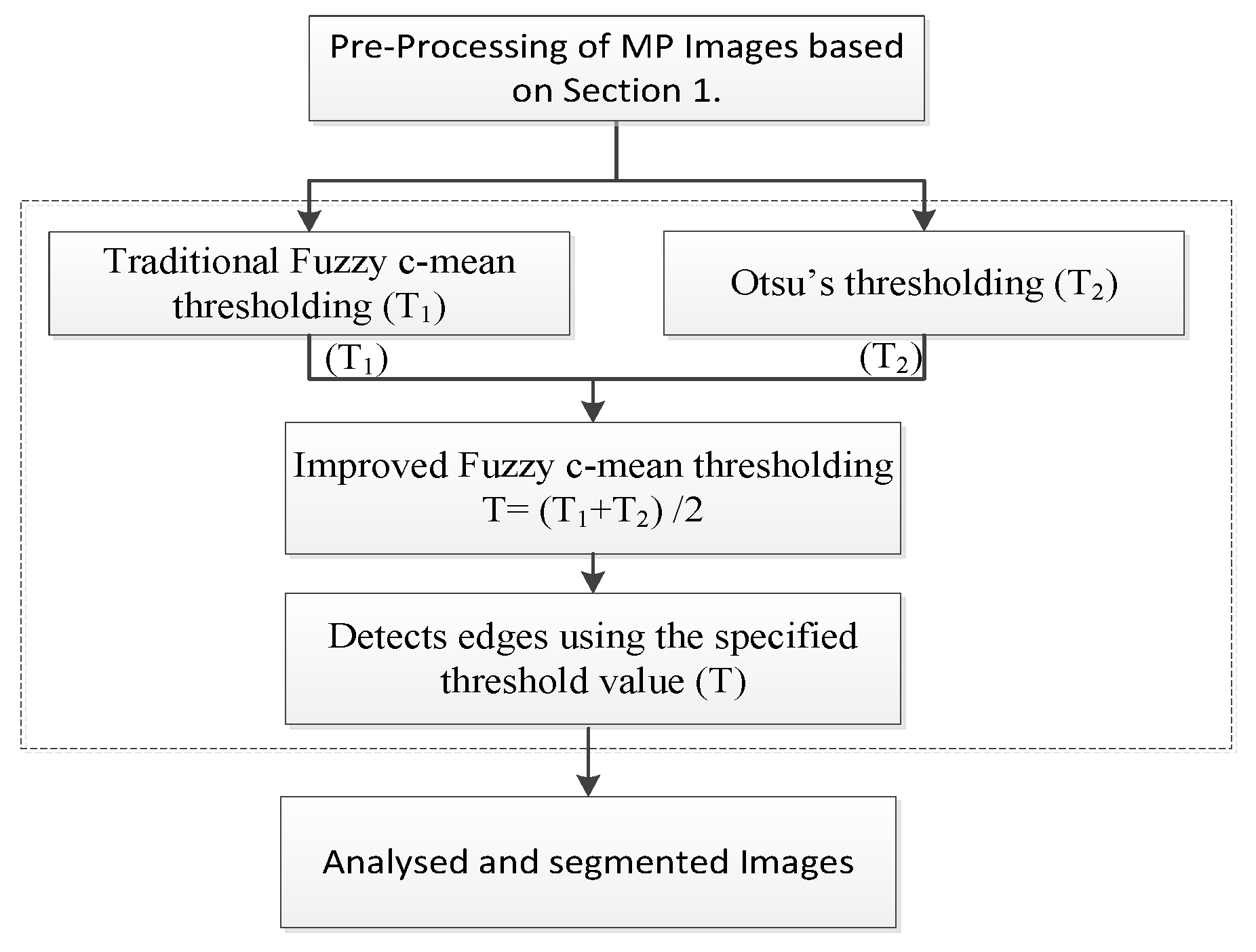
Figure 1.
Flowchart of the developed Fuzzy c-mean thresholding algorithm.
Figure 1.
Flowchart of the developed Fuzzy c-mean thresholding algorithm.
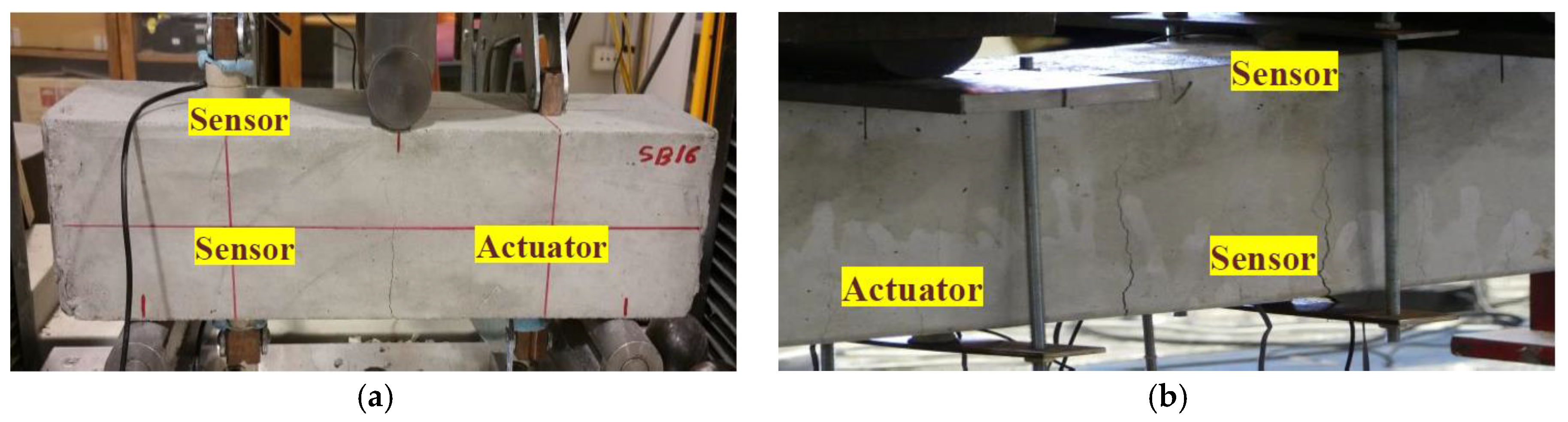
Figure 2.
Bending test set up: (a) concrete, (b) RC beam.
Figure 2.
Bending test set up: (a) concrete, (b) RC beam.
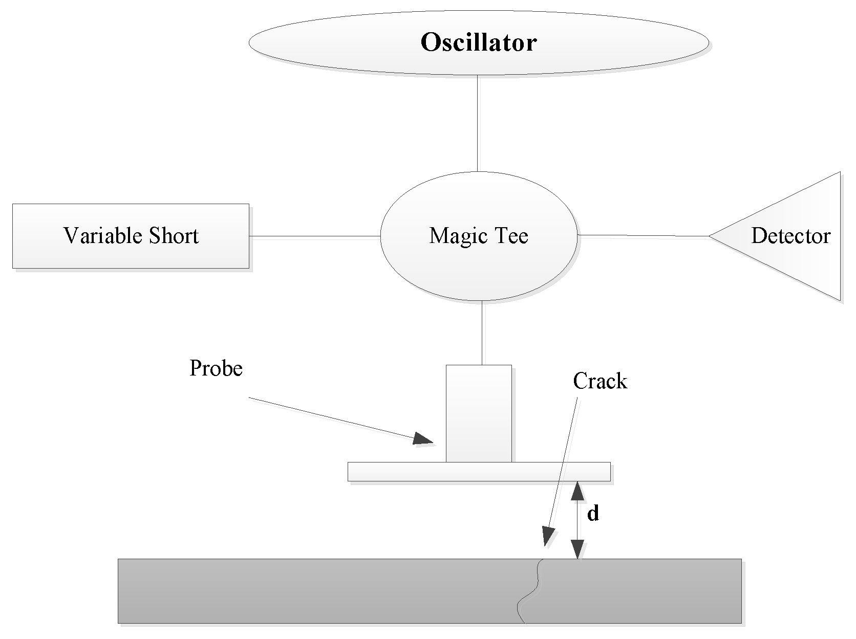
Figure 3.
Measurement setup.
Figure 3.
Measurement setup.
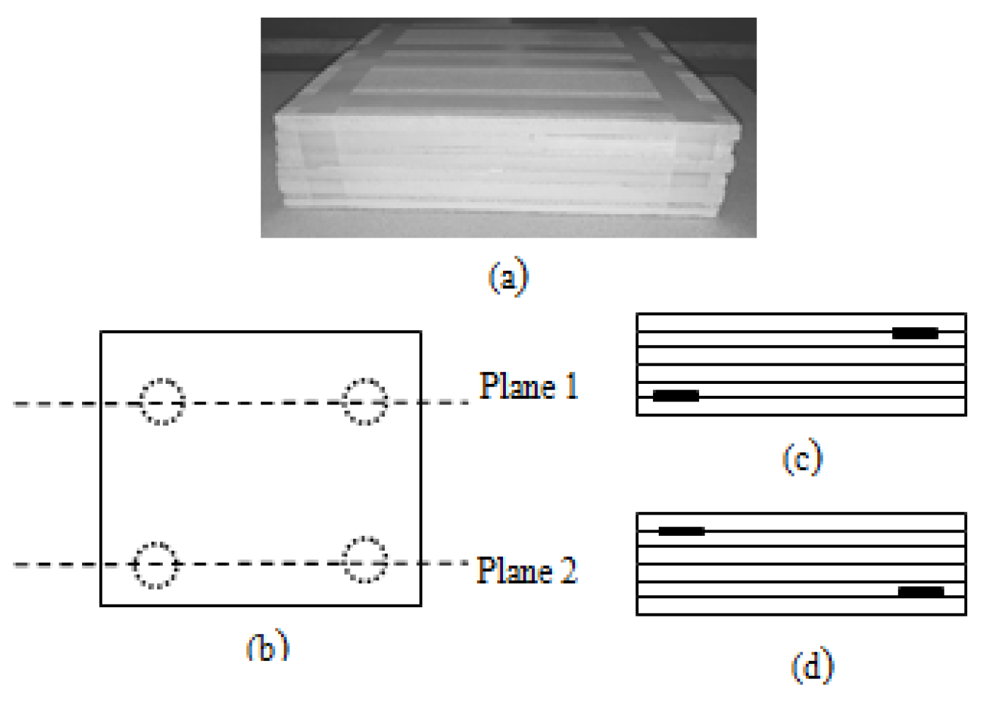
Figure 4.
(a) Picture and schematic of (b) the top view, with the embedded disks indicated, (c) the cross-sectional side view at Plane 1, and (d) the cross-sectional side view at Plane 2.
Figure 4.
(a) Picture and schematic of (b) the top view, with the embedded disks indicated, (c) the cross-sectional side view at Plane 1, and (d) the cross-sectional side view at Plane 2.
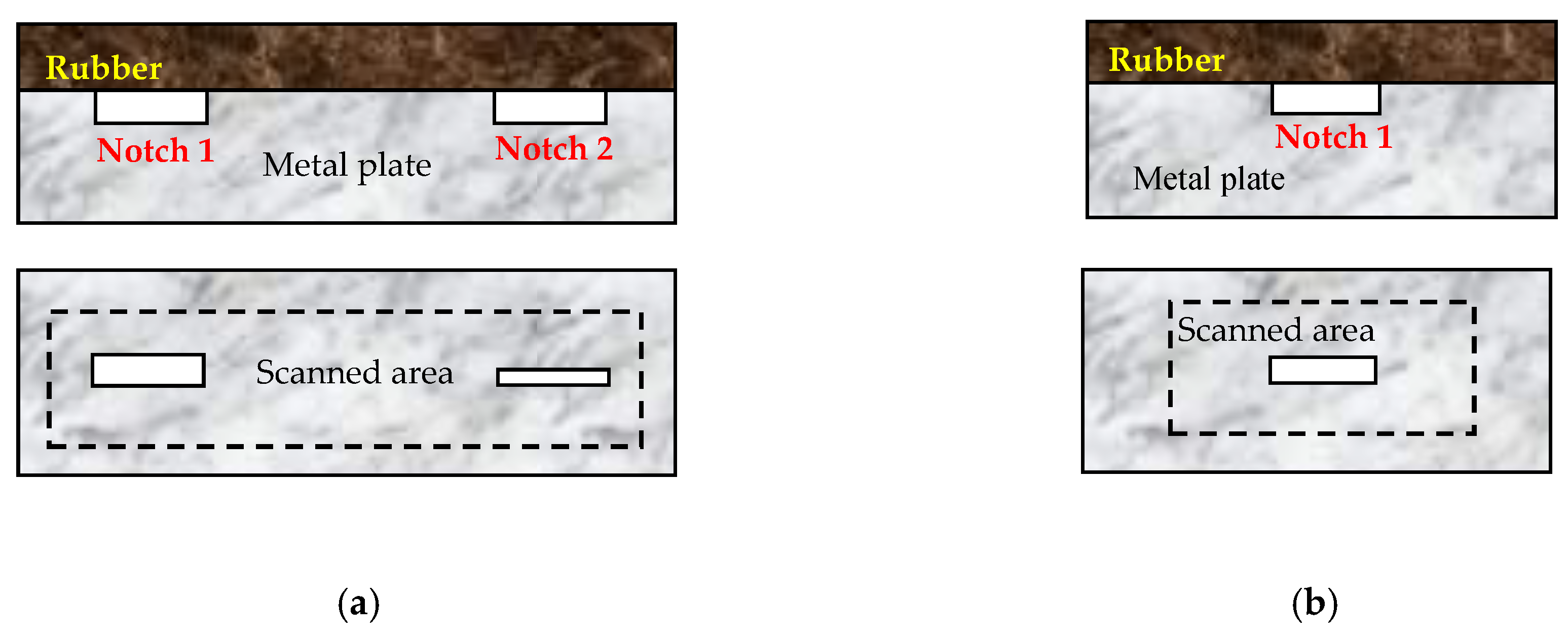
Figure 5.
Cross-sectional side view (upper) and schematic of the top view without the rubber layer (lower) of the parts of aluminum plate with (a) notch 1 and (b) notches 1 and 2.
Figure 5.
Cross-sectional side view (upper) and schematic of the top view without the rubber layer (lower) of the parts of aluminum plate with (a) notch 1 and (b) notches 1 and 2.
Figure 6.
Signals recorded under 50 × 70 scanning, obtained at three standoff distances: (a) 0.2 mm, (b) 0.8 mm, and (c) 1.7 mm.
Figure 6.
Signals recorded under 50 × 70 scanning, obtained at three standoff distances: (a) 0.2 mm, (b) 0.8 mm, and (c) 1.7 mm.
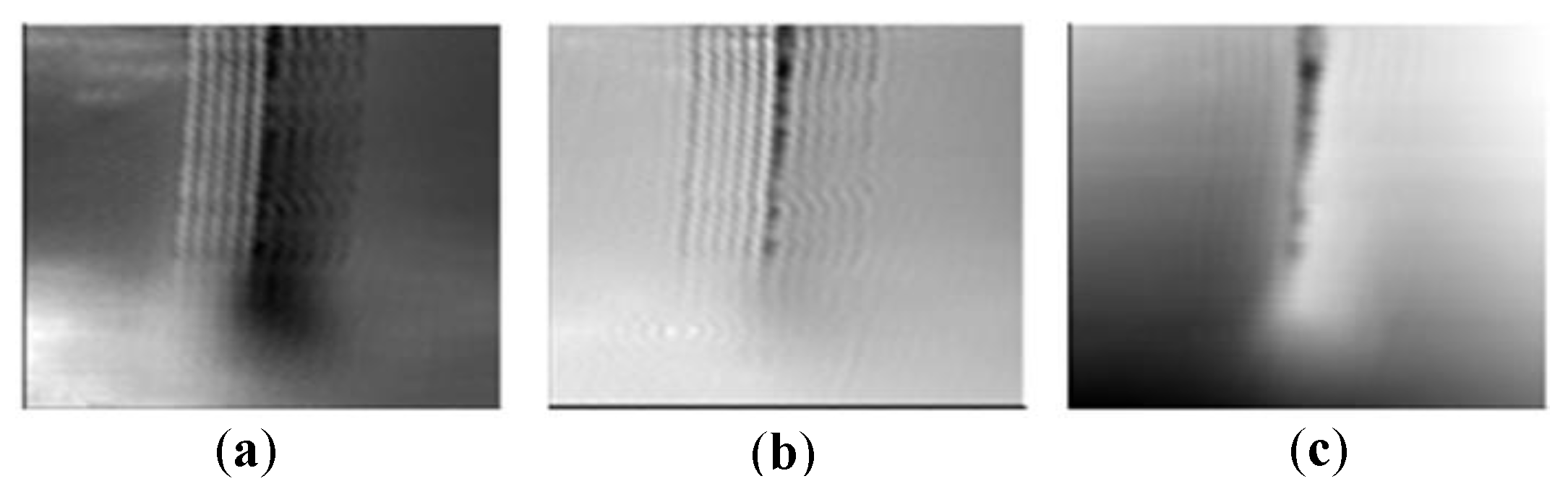
Figure 7.
Original images of the portion of the covered crack under 50 × 70 scanning, obtained at three standoff distances: (a) 0.2 mm, (b) 0.8 mm, and (c) 1.7 mm.
Figure 7.
Original images of the portion of the covered crack under 50 × 70 scanning, obtained at three standoff distances: (a) 0.2 mm, (b) 0.8 mm, and (c) 1.7 mm.
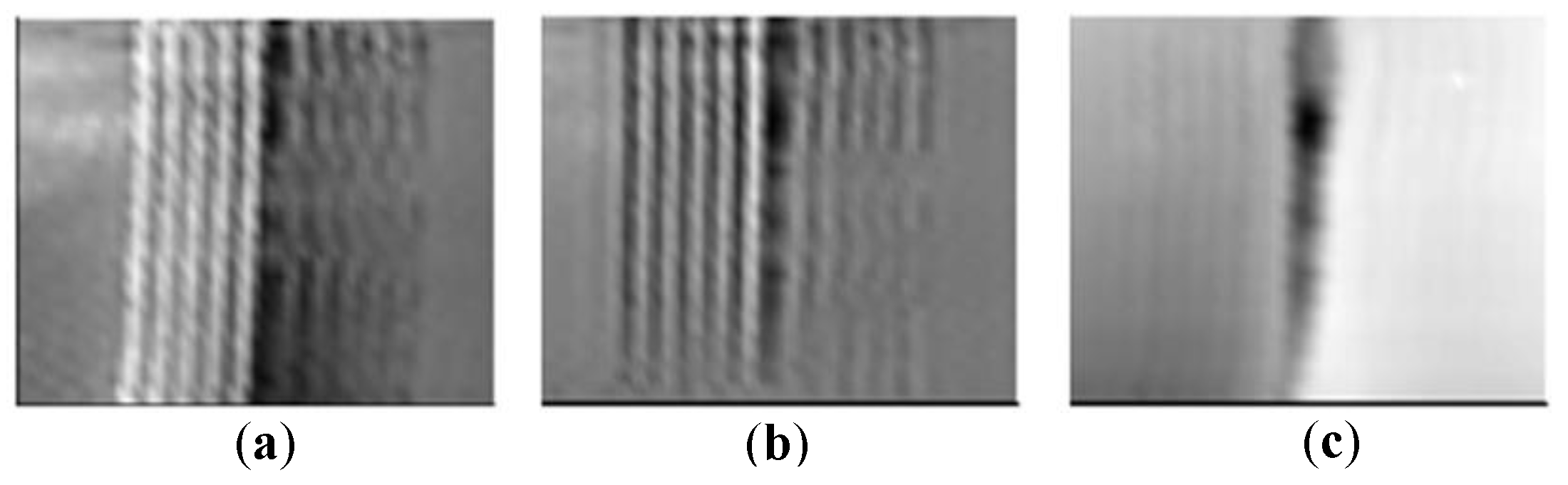
Figure 8.
Original images of the portion of the covered crack under 30 × 30 scanning, obtained at three standoff distances: (a) 0.2 mm, (b) 0.8 mm, and (c) 1.7 mm.
Figure 8.
Original images of the portion of the covered crack under 30 × 30 scanning, obtained at three standoff distances: (a) 0.2 mm, (b) 0.8 mm, and (c) 1.7 mm.
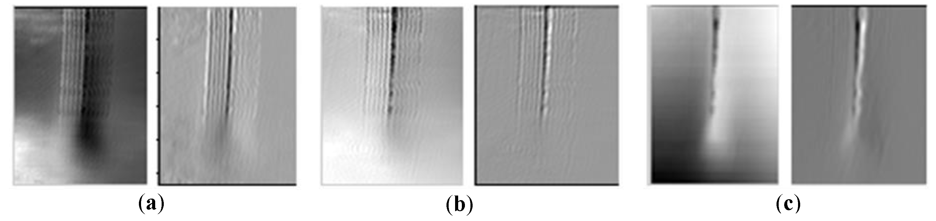
Figure 9.
(a) Left: Original image with d ~ 1.7, (a) Right: Enhanced image with d ~ 1.7, (b) Left: Original image with d ~ 0.8, (b) Right: Enhanced image with d ~ 0.8 (c) Left: Original image with d ~ 0.2, (c) Right: Enhanced image with d ~ 0.2 mm.
Figure 9.
(a) Left: Original image with d ~ 1.7, (a) Right: Enhanced image with d ~ 1.7, (b) Left: Original image with d ~ 0.8, (b) Right: Enhanced image with d ~ 0.8 (c) Left: Original image with d ~ 0.2, (c) Right: Enhanced image with d ~ 0.2 mm.
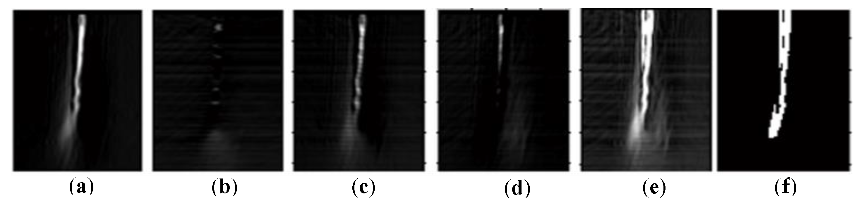
Figure 10.
(a) Gradient in the x-direction (b) Gradient in the y-direction (c) Gradient in the d1 direction, (d) Gradient in the d2 direction, (e) Gradient magnitude, (f) Otsu’s thresholding.
Figure 10.
(a) Gradient in the x-direction (b) Gradient in the y-direction (c) Gradient in the d1 direction, (d) Gradient in the d2 direction, (e) Gradient magnitude, (f) Otsu’s thresholding.
Figure 11.
2D grid coordinates of segmented image.
Figure 11.
2D grid coordinates of segmented image.
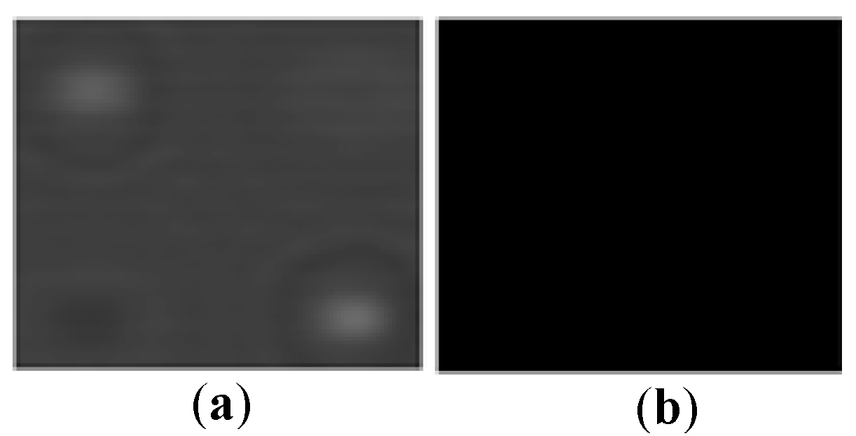
Figure 12.
Microwave image of the sample for the composite material: (a) magnitude and (b) phase.
Figure 12.
Microwave image of the sample for the composite material: (a) magnitude and (b) phase.
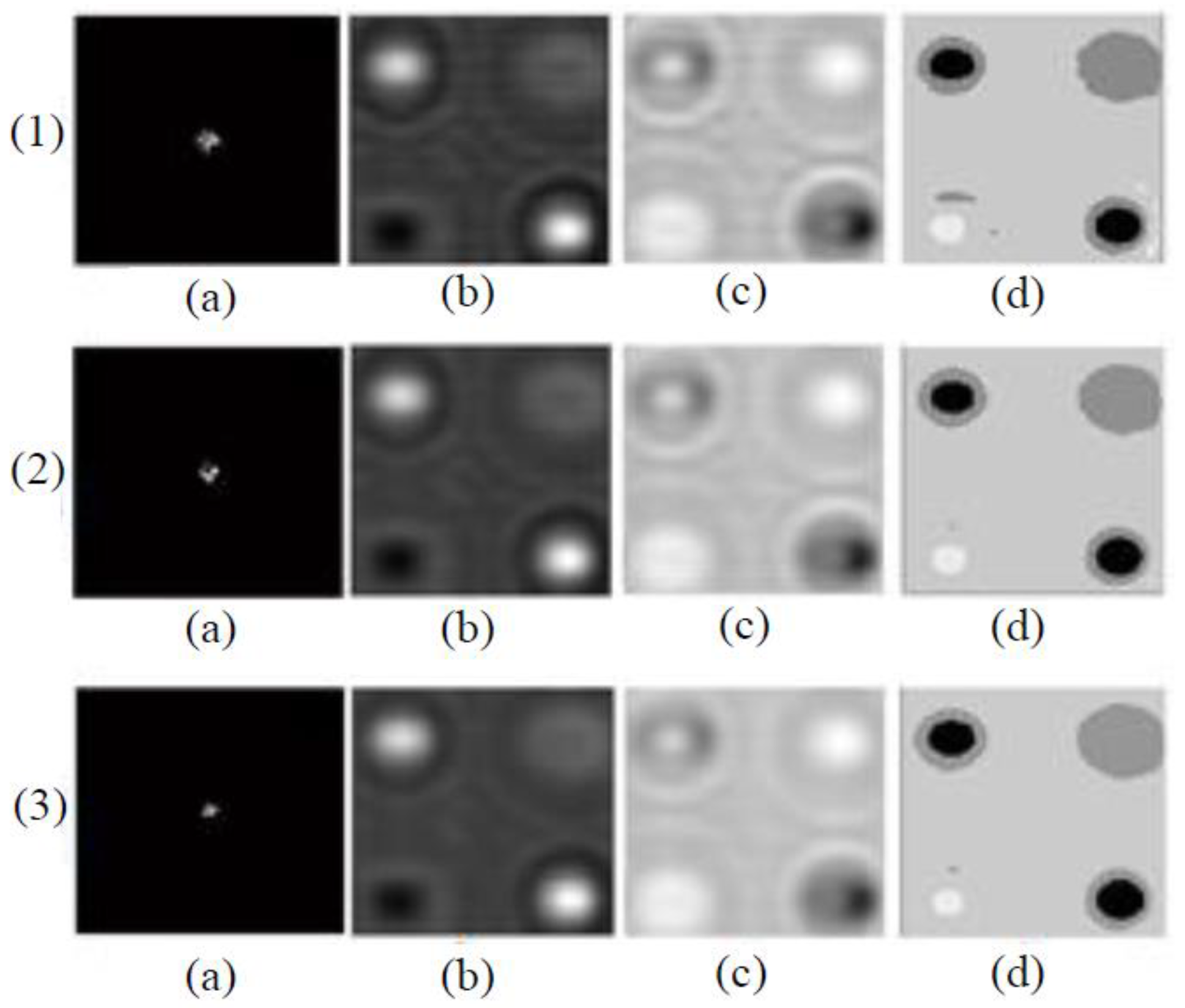
Figure 13.
The total process of target segmentation of the sample, using Fourier transform and Wavelet transform, followed by Multi-thresholding and erosion, with (1) single, (2) two-fold, and (3) three-fold multiplications, (a) Fourier transforms, (b) inverted Fourier transforms (magnitude), (c) inverted Fourier transforms (phase), and (d) segmented results.
Figure 14.
The total process of target segmentation of sample using Fourier transform and Gaussian followed by Multi-thresholding and erosion, with (1) single-, (2) two-fold, and (3) three-fold multiplications, (a) Fourier transforms, (b) inverted Fourier transforms (magnitude), (c) inverted Fourier transforms (phase), and (d) segmented results.
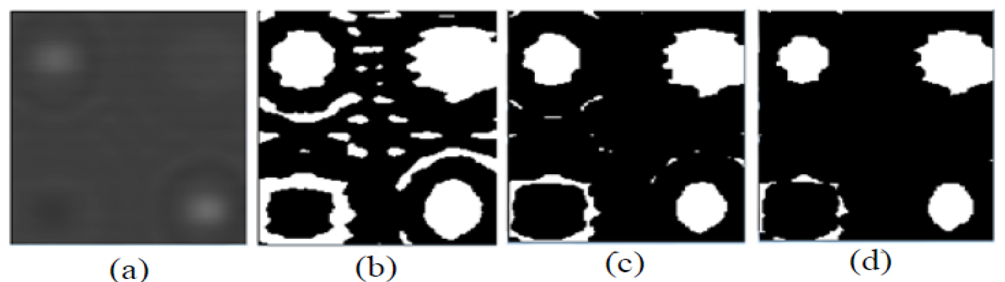
Figure 15.
Images of the sample, showing the total process of target segmentation, using fuzzy c-mean clustering, followed by multi-thresholding and erosion, (a) original image, (b) fuzzy c-mean clustering, (c) erosion by structuring element object 10, and (d) erosion by structuring element object 15.
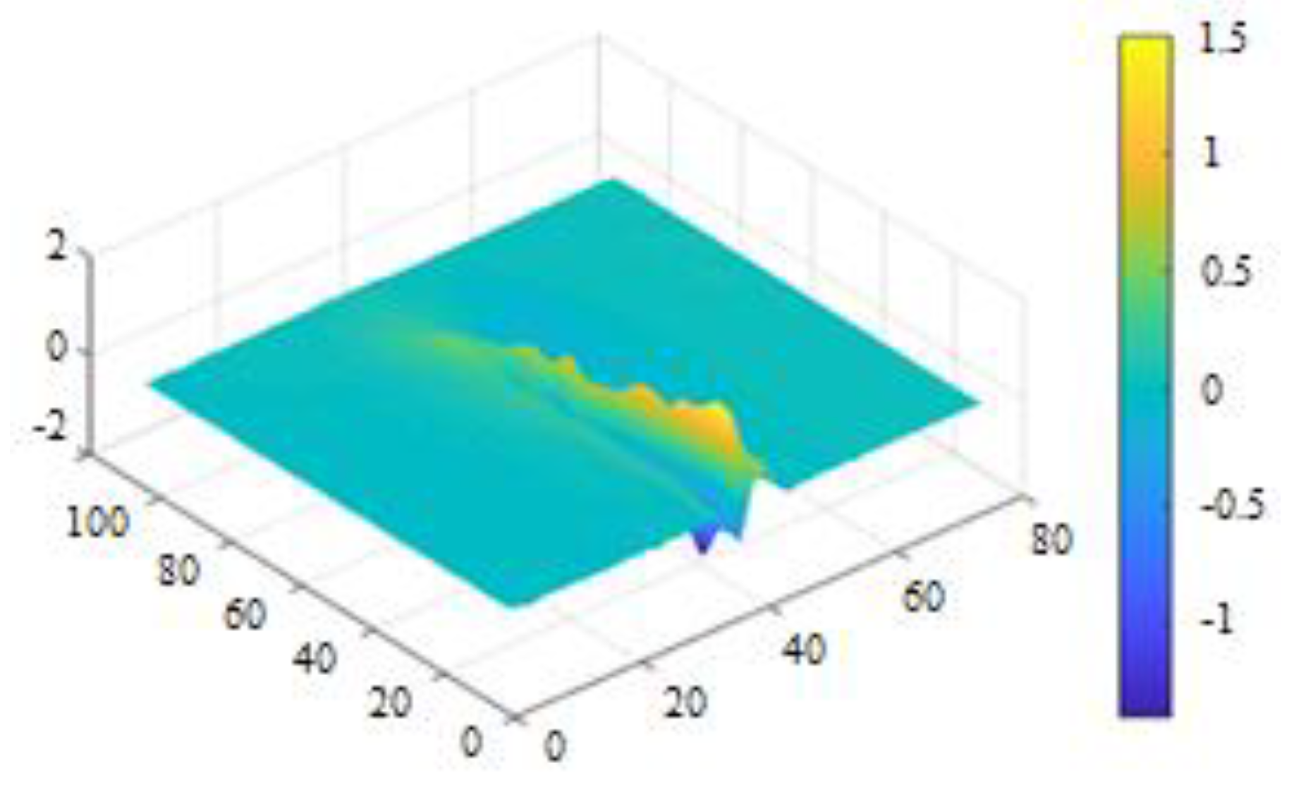
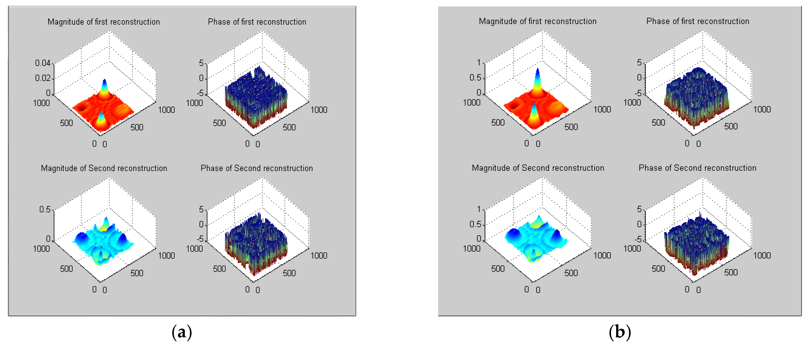
Figure 16.
3D demonstration of the phase and magnitude of the 2D data, (a) a reconstructed image based on a wavelet transform, and (b) a reconstructed image based on a Gaussian transform.
Figure 16.
3D demonstration of the phase and magnitude of the 2D data, (a) a reconstructed image based on a wavelet transform, and (b) a reconstructed image based on a Gaussian transform.
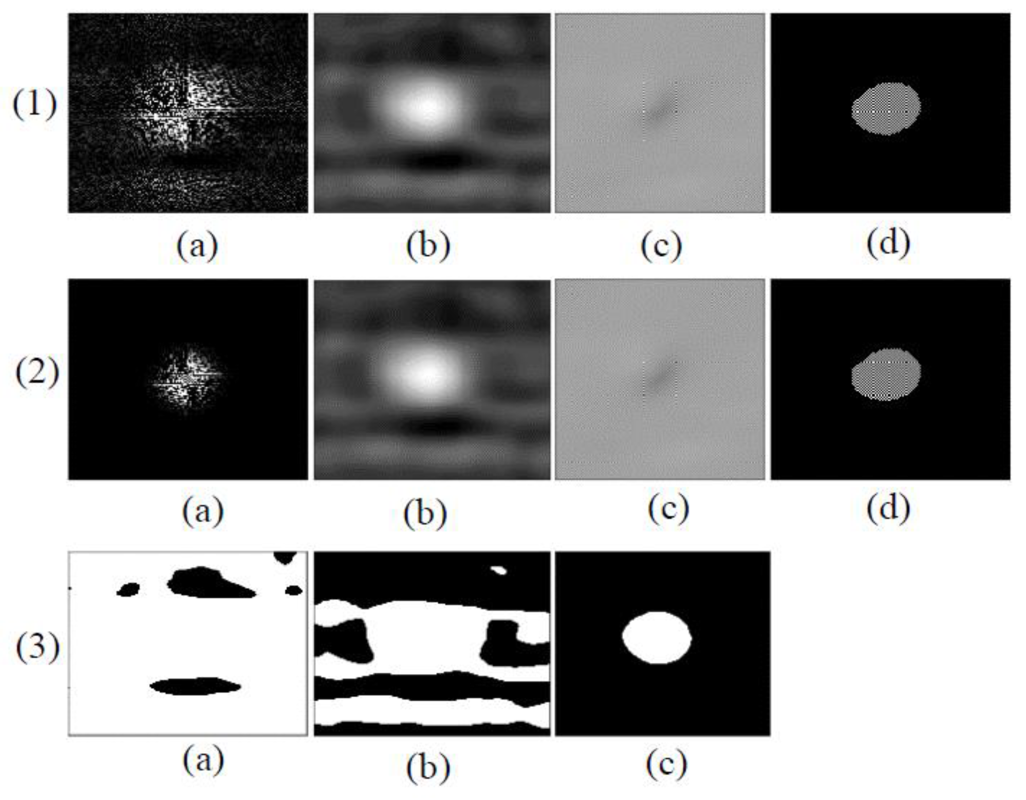
Figure 17.
The total process of target segmentation using (1) Fourier transform and Wavelet transform, followed by multi-thresholding and erosion, (2) Fourier transform and Gaussian, followed by multi-thresholding and erosion, (a) Fourier transforms, (b) inverted Fourier transforms (magnitude), (c) inverted Fourier transforms (phase), and (d) segmented results, and (3) a fuzzy c-mean algorithm with, (a) a threshold value of 0.206500, (b) a threshold value of 0.211538, and (c) a threshold value of 0.480769.
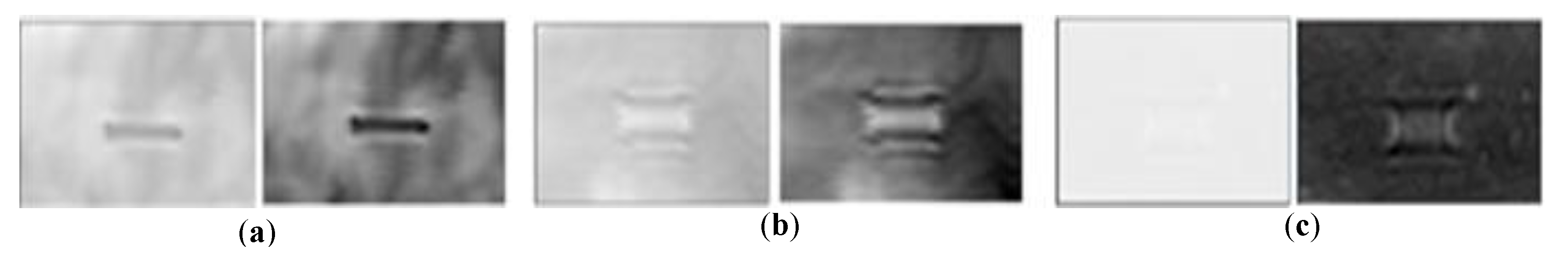
Figure 18.
Original (left) and enhanced (right) images of notch 1 under the 2 mm-thick rubber layer, obtained at three standoff distances: (a) 0.1 mm, (b) 0.25 mm, and (c) 4 mm.
Figure 18.
Original (left) and enhanced (right) images of notch 1 under the 2 mm-thick rubber layer, obtained at three standoff distances: (a) 0.1 mm, (b) 0.25 mm, and (c) 4 mm.
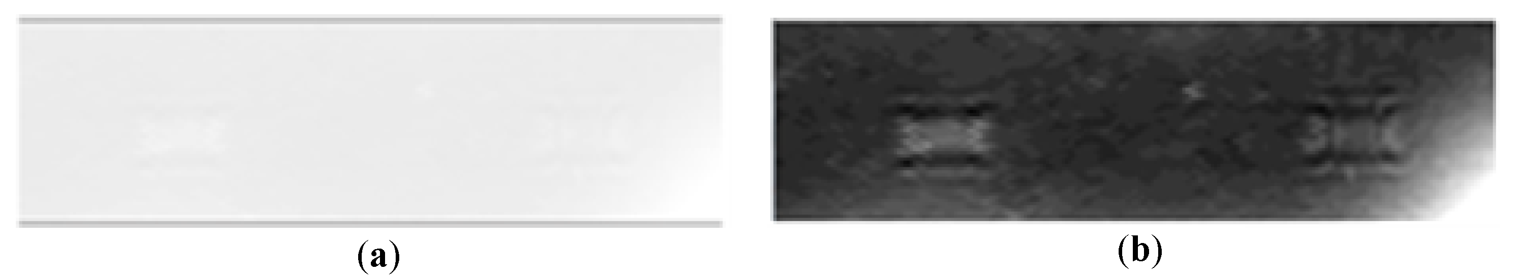
Figure 19.
The (a) original and (b) enhanced images of notches 1 and 2 under the 4 mm-thick rubber layer, obtained at a standoff distance of 0.1 mm.
Figure 19.
The (a) original and (b) enhanced images of notches 1 and 2 under the 4 mm-thick rubber layer, obtained at a standoff distance of 0.1 mm.
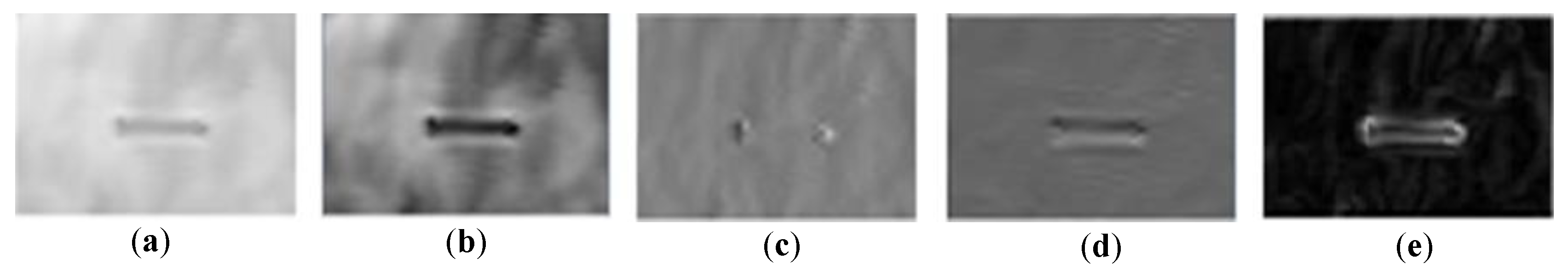
Figure 20.
Images of notch 1 under the 2 mm-thick rubber layer obtained at a standoff distance of 0.1 mm: (a) original and after (b) average filtering, (c) gradient filtering in the x-direction (, (d) gradient filtering in the y-direction ( and (e) gradient magnitude with the Sobel method, .
Figure 20.
Images of notch 1 under the 2 mm-thick rubber layer obtained at a standoff distance of 0.1 mm: (a) original and after (b) average filtering, (c) gradient filtering in the x-direction (, (d) gradient filtering in the y-direction ( and (e) gradient magnitude with the Sobel method, .
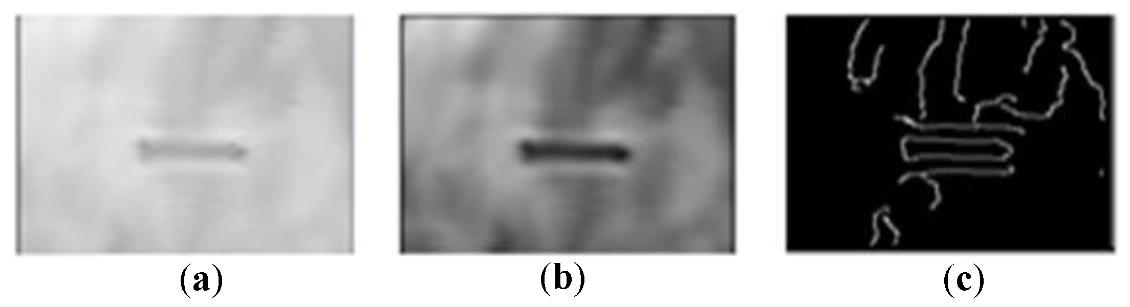
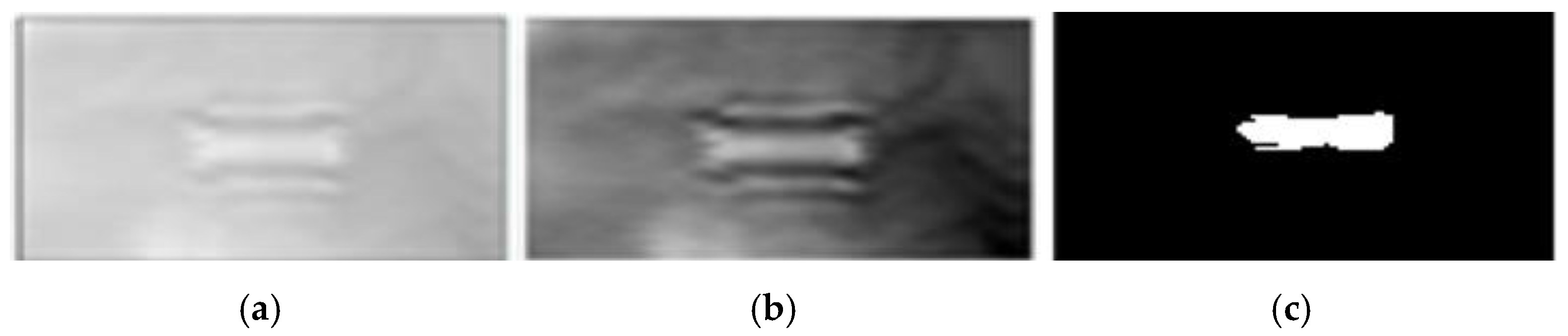
Figure 21.
Images of notch 1 under the 2 mm-thick rubber layer: (a) original and after (b) average filtering, (c) the canny edge detection algorithm obtained at a standoff distance of 0.1 mm.
Figure 21.
Images of notch 1 under the 2 mm-thick rubber layer: (a) original and after (b) average filtering, (c) the canny edge detection algorithm obtained at a standoff distance of 0.1 mm.
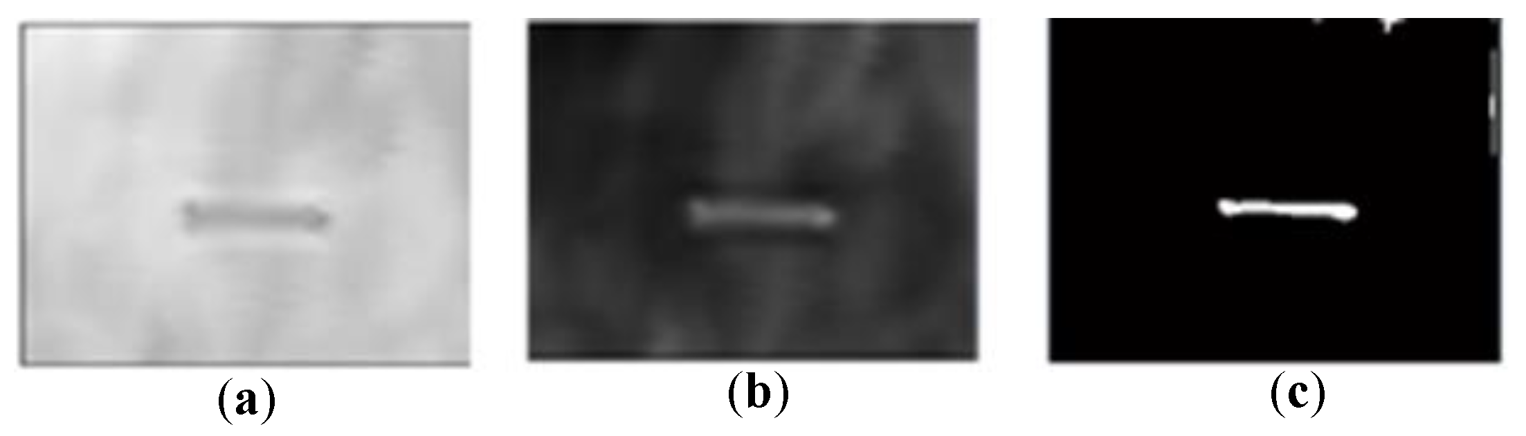
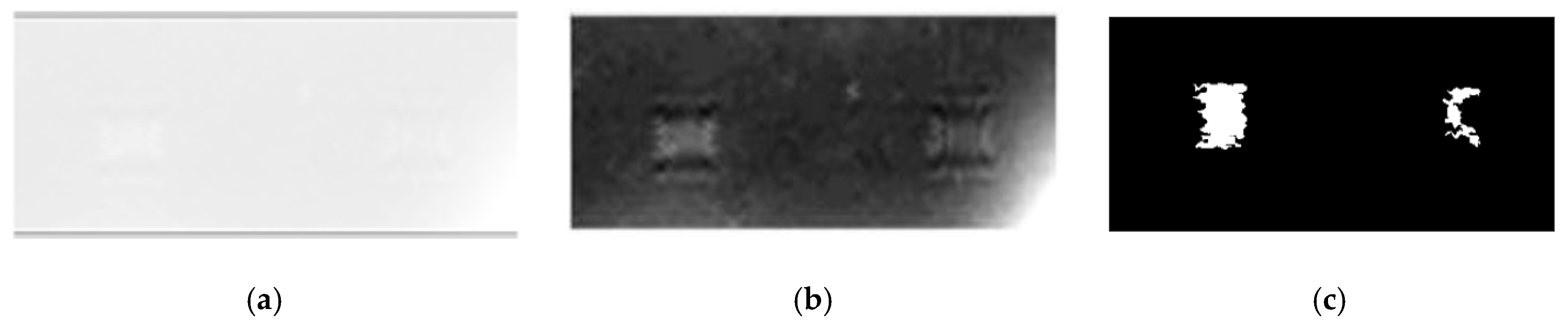
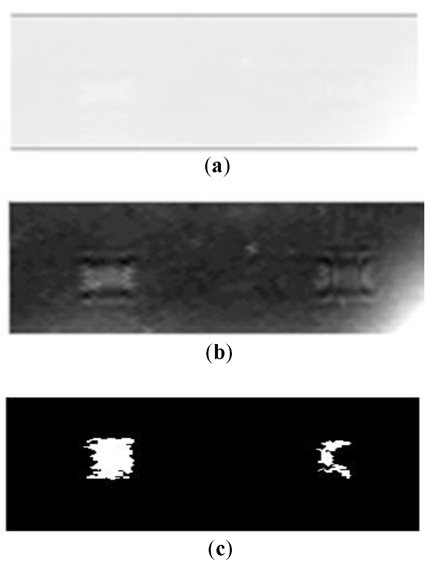
Figure 22.
Images of notch 1 under the 2 mm-thick rubber layer obtained at a standoff distance of 0.1 mm: (a) original and after (b) average filtering, and (c) thresholding by the developed fuzzy c-mean thresholding algorithm.
Figure 22.
Images of notch 1 under the 2 mm-thick rubber layer obtained at a standoff distance of 0.1 mm: (a) original and after (b) average filtering, and (c) thresholding by the developed fuzzy c-mean thresholding algorithm.
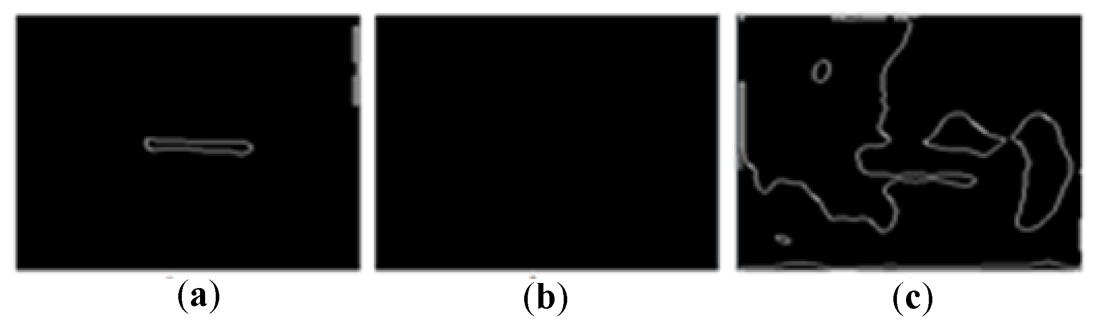
Figure 23.
Notch edge detection, obtained with the (a) gradient magnitude, using Sobel’s gradient, (b) Canny edge detection algorithm, and (c) the developed fuzzy c-mean thresholding algorithm.
Figure 23.
Notch edge detection, obtained with the (a) gradient magnitude, using Sobel’s gradient, (b) Canny edge detection algorithm, and (c) the developed fuzzy c-mean thresholding algorithm.
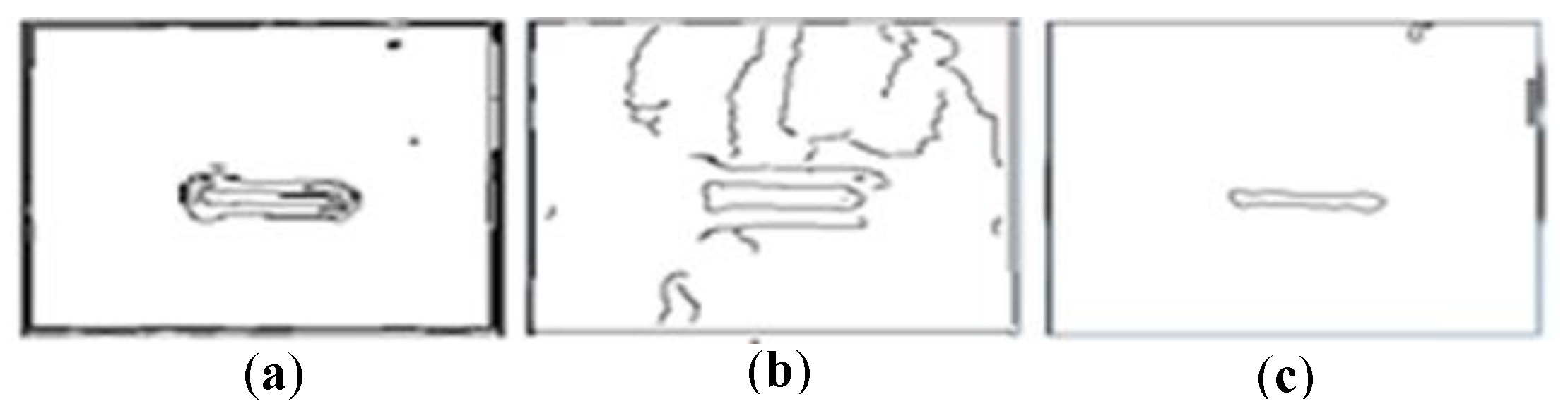
Figure 24.
Notch edge detection, obtained with (a) the developed fuzzy c-mean thresholding algorithm, (b) the traditional fuzzy c-mean thresholding algorithm, and (c) Otsu’s thresholding algorithm.
Figure 24.
Notch edge detection, obtained with (a) the developed fuzzy c-mean thresholding algorithm, (b) the traditional fuzzy c-mean thresholding algorithm, and (c) Otsu’s thresholding algorithm.
Table 1.
Specifications for experimental setup.
Table 1.
Specifications for experimental setup.
| Concrete Beam | Size (mm) | Loading Capacity (kN) | Displacement Movement (mm/min) | Loading Cell Starting Point |
|---|
| Simple | 400 × 100 × 100 | 200 | 0.01 | 0 |
| Reinforced | 1700 × 150 × 250 | 1000 | 0.009 | 0 |
Table 2.
Comparison of accuracy between the traditional and the developed Support Vector Machine (SVM).
Table 2.
Comparison of accuracy between the traditional and the developed Support Vector Machine (SVM).
| Accuracy (%) |
|---|
| No. Observations | Concrete Beam | RC Beam |
|---|
| Simple SVM | Developed SVM | Simple SVM | Developed SVM |
|---|
| 1 | 84.72 | 87.23 | 85.26 | 86.19 |
| 2 | 84.63 | 87.19 | 85.42 | 87.14 |
| 3 | 84.81 | 87.22 | 85.39 | 86.19 |
| 4 | 84.76 | 87.23 | 85.4 | 86.18 |
| 5 | 84.83 | 87.19 | 85.39 | 86.15 |
| 6 | 84.46 | 87.23 | 85.28 | 86.19 |
| 7 | 84.91 | 87.22 | 85.2 | 86.5 |
| 8 | 84.63 | 87.24 | 85.48 | 86.19 |
| 9 | 84.65 | 87.35 | 85.4 | 86.19 |
| 10 | 84.61 | 87.22 | 85.52 | 86.56 |
| 11 | 84.91 | 87.2 | 85.38 | 86.25 |
| 12 | 84.52 | 87.18 | 85.29 | 86.19 |
| 13 | 84.66 | 87.2 | 85.43 | 86.66 |
| 14 | 84.87 | 87.21 | 85.29 | 86.16 |
| 15 | 84.8 | 87.21 | 85.42 | 86.18 |
| 16 | 84.81 | 87.19 | 85.46 | 86.19 |
| 17 | 84.82 | 87.23 | 85.44 | 86.12 |
| 18 | 84.58 | 87.23 | 85.31 | 86.19 |
| 19 | 84.88 | 87.22 | 85.27 | 86.19 |
| 20 | 84.76 | 87.23 | 85.44 | 86.21 |
| 21 | 84.55 | 87.23 | 85.32 | 86.19 |
| 22 | 84.8 | 87.28 | 85.43 | 86.38 |
| 23 | 84.65 | 87.19 | 85.32 | 86.19 |
| 24 | 84.6 | 87.17 | 85.37 | 86.19 |
| 25 | 84.87 | 87.19 | 85.47 | 86.47 |
| 26 | 84.58 | 87.22 | 85.45 | 86.19 |
| 27 | 84.83 | 87.22 | 85.24 | 86.72 |
| 28 | 84.93 | 87.35 | 85.42 | 86.14 |
| 29 | 84.68 | 87.19 | 85.4 | 86.19 |
| Average | 84.72 | 87.22 | 85.38 | 86.29 |
Table 3.
T-Test: Simple SVM and developed SVM sample for the means.
Table 3.
T-Test: Simple SVM and developed SVM sample for the means.
| | Simple SVM | Developed SVM |
|---|
| Mean | 84.73 | 87.22 |
| Observations | 29 | 29 |
| t statistic | −101.443 | |
| P (T ≤ t), one-tailed | 8.78×10⁻³ | |
| P (T ≤ t) two-tail | 1.76×10⁻³ | |
Table 4.
Properties of the image region, results, and descriptions.
Table 4.
Properties of the image region, results, and descriptions.
| Property | Result | Description |
|---|
| Centroid | [38.7045 27.9205] | Mass center of the region |
| BoundingBox | [35.5000 2.5000 7 64] | Smallest rectangle containing the region |
| FilledImage | [64 × 7 logical] | Image with the size of bounding box for the region |
| FilledArea | 176 | Number of ‘on’ pixels |
| MajorAxisLength | 68.7051 | Number of pixels for the major axis of the ellipse |
| MinorAxisLength | 5.8664 | Number of pixels for the minor axis of the ellipse |
| Orientation | 88.0654 (degree) | Angle between the MajorAxisLength and the x-axis |


