Scale-Free Features in Collective Robot Foraging

Abstract

In many complex systems observed in nature, properties such as scalability, adaptivity, or rapid information exchange are often accompanied by the presence of features that are scale-free, i.e., that have no characteristic scale. Following this observation, we investigate the existence of scale-free features in artificial collective systems using simulated robot swarms. We implement a large-scale swarm performing the complex task of collective foraging, and demonstrate that several space and time features of the simulated swarm—such as number of communication links or time spent in resting state—spontaneously approach the scale-free property with moderate to strong statistical plausibility. Furthermore, we report strong correlations between the latter observation and swarm performance in terms of the number of retrieved items.

1. Introduction

Advances in computation have made it possible to record, simulate, and analyze multi-agent complex systems in nature, such as fish schools, bird flocks, locust swarms, and ant colonies. In many of these collective systems, various attributes were found to be scale-free [1], i.e., the attributes do not have a characteristic size or value. Examples of such scale-free features found in biological systems include, among others, (i) asymptotically scale-free correlation lengths of starling flocks [2,3]—the term asymptotic refers to the behavior of a variable (in this case spatial correlation) close to a limit (in this case an infinite flock size); (ii) scale-free fluctuations of velocity and orientation correlations in moving bacterial colonies [4]; (iii) time intervals between communication calls that follow a power law—which is the mathematical representation of a scale-free property—in pairs of zebra finches; and (iv) scale-free movement patterns found in models of foraging primates [5] or midge swarms [6].

One of the most prominent findings is that the number of interactions appear to be scale-free in various real-world networks of biological and social systems [7,8,9]. Multi-agent systems benefit from scale-free communication because it enables scalable, fast and efficient information transfer [10,11,12]. An essential aspect of scale-free networks is that they represent complex topologies in which only a few nodes (called hubs) have a comparably high connectivity degree [7]. This small percentage of highly connected hubs makes scale-free topologies vulnerable to targeted attacks but exceptionally robust to random failures (which are likely to affect the vast majority of nodes that are not hubs) [13]. Furthermore, due to the high connectivity, the network diameter is small, which means that on average, any two nodes can share their information only over a few hops [11], resulting in fast information transfer.

Inspired by the high prevalence of scale-free features in (socio-) biological systems, the aim of the current study is to examine whether scale-free attributes may also spontaneously emerge in artificial collective systems. One particularly prominent example of these systems inspired by nature is swarm robotics, where robot collaboration is an essential prerequisite for the successful execution of tasks [14,15,16,17,18,19,20]. Although accurate understanding and systematic design of swarm robotic systems are considered to be among the greatest challenges of contemporary robotics [21], swarm robotics benefits strongly from the progress made in wireless communication technologies, system integration, machine learning and artificial intelligence (AI). Consequently, artificial cooperative multi-agent systems gain in importance not only in applied science and engineering but also in fundamental research, allowing the shrinkage of the reality gap of detailed modeling and the accurate simulation of distributed biological systems.

Many natural collective behaviors were modeled using artificial collective systems, including bird flocking [22], locust marching [23] or cockroach aggregation [24]. However, among the most prominent challenges is the collective foraging task [18]. Extensive efforts were dedicated to the study of the foraging task because of its remarkable prevalence. The foraging behavior is found in various species and subspecies across the world [25,26]. In most cases, its efficient implementation is essential to group survival.

In essence, a multi-agent system performing the foraging task has the goal of collectively retrieving information and other resources from the environment. Different to a single-agent implementation, the benefit of a multi-agent system is its ability to share the accessed resources and information to enhance the overall performance. However, the multi-agent foraging task exhibits a considerable degree of complexity, making its modeling and analysis very demanding [18]. Successful collective foraging often requires a delicate combination of several extensively studied multi-agent sub-behaviors such as deployment [27,28], exploration [29,30], aggregation [31,32] or information sharing [33,34]. Hence, even though collective foraging itself can be considered to be a specific task within a large class of multi-agent problems, it rightfully receives separate attention in numerous contemporary studies [16,35,36,37,38].

Moreover, collective foraging is a promising behavior for many real-world applications such as exploration by aerial vehicles [39], underwater monitoring [40], or optimization of electrical networks [41]. Therefore, the foraging performance of artificial multi-agent systems, potentially in combination with other types of AI, is worthwhile investigating in depth. In particular, in robot swarms, various fundamental questions have already been addressed such as the influence of interference [42,43], regulation of information flow [33] or achievement of consensus [44]. Nevertheless, other relevant questions are still open to research, including how does the distribution of individual features change in relation to the input from the environment or social interactions? Is there a connection between particular feature distributions and the performance of the swarm? To address these questions with respect to scale-free properties, we simulate the foraging behavior in a robot swarm and analyze the emergence of scale-free features. For this purpose, the complexity of the foraging task is advantageous as it offers a wide range of features that can be examined for their statistical tendency to be scale-free.

Our goal can be split into the following: (i) investigating the existence of scale-free features in a robot swarm performing the foraging task, (ii) studying the correlation between these features and the swarm performance, (iii) discussing the potential role of feedback mechanisms in the emergence of such scale-free features.

We begin with defining the robot (microscopic) and the swarm (macroscopic) behaviors in Section 2.1 and Section 2.2, respectively. The link between these two levels of behaviors is formulated using statistical distributions and elaborated on in Section 2.4. In Section 2.5, we describe the experimental setup. Thereafter, in Section 3 we demonstrate the occurrence of scale-invariant features—such as those related to the communication degree or times spent in foraging or resting—and their correlation with swarm performance. Furthermore, we discuss the present feedback mechanisms that may support the emergence of scale-free features in a sophisticated set of scenario configurations. Lastly, the paper is concluded in Section 4.

2. Methods

2.1. Robot Behavior

We focus on the robot’s decision-making process that is defined by the robot’s interactions and the robot’s individual preferences. The robots are situated in an arena which consists of a nest and a foraging area. Each robot can switch between two states: resting and exploring. In biology, similar behavior called forager activation has been observed in harvester ants, Pogonomyrmex barbatus, and reported in several publications [45,46,47]. In the exploring state, the robot moves around searching for items—which are located only in the foraging area—to retrieve to the nest. The robot moves on a straight line until it encounters another robot or a wall, in which case a collision avoidance maneuver is initiated. In the resting state, the robot rests inside the nest and only in this state it is allowed to communicate with the neighbors within its line of sight. Specifically, each robot can broadcast a message about the success or failure of its latest exploration attempt or listen to its neighbors. Received information may either increase or decrease the robot’s probability to switch from resting to exploring or vice versa. Probabilities are updated continuously using fixed probability jumps—we refer to those by the term cues, as in [14]. In the following, we introduce the different probability cues used in implementing the foraging behavior, in addition to the probabilities determining the switch between the two robot states. We also consider two distinct communication modes defining the duration of information exchange.

2.1.1. State Switching Probabilities

Following [14], there is a minimum duration θ for the robot to stay in a certain state. The purpose of having such a threshold is to ensure that robots can perform the sub-tasks associated with this state for a certain amount of time so that necessary dynamics can take place. For instance, a minimum exploring time θ_e needs to be at least as long as it takes for a robot to reach the most remote items (taking into account the constant linear speed of that robot) [16].

With this in mind, let us formulate the individual response to social and environmental cues in terms of switching probabilities. We denote $\left\{i_e,i_r\right\}\in \left\{{\mathbb{R}}_0^{+},{\mathbb{R}}_0^{+}\right\}$ and $\left\{s_e,s_r\right\}\in \left\{{\mathbb{R}}_0^{+},{\mathbb{R}}_0^{+}\right\}$ as the robot’s internal (i) and social (s) cues to switch to exploring (e) or resting (r) state, respectively. The probability of a robot to switch from the resting state to the exploring state is denoted by $p_{r\to e}$, whereas the probability to switch from the exploring state to the resting state is denoted by $p_{e\to r}$.

The probabilities are updated iteratively at every simulation time step in a discrete manner as in the following:

$$\begin{array}{cc}\hfill p_{r\to e}(t+1)& =p_{r\to e}\left(t\right)+{\delta }_{\eta }\left(t\right)s_e+{\delta }_{\varphi }\left(t\right)i_e\hfill \end{array}$$

(1)

$$\begin{array}{cc}\hfill p_{e\to r}(t+1)& =p_{e\to r}\left(t\right)-{\delta }_{\eta }\left(t\right)s_r-{\delta }_{\varphi }\left(t\right)i_r,\hfill \end{array}$$

(2)

where ${\delta }_{\eta }\left(t\right)$ is the number of ‘success’ minus ‘failure’ messages received by the robot from its neighbors at every time step spent in the resting state. Additionally, the robot’s own experience is characterized using ${\delta }_{\varphi }\left(t\right)$. This is defined for every exploration attempt as follows:

$${\delta }_{\varphi }\left(t\right)=\left\{\begin{array}{cc}+1,\hfill & \mathrm{at}\mathrm{the}\mathrm{time}\mathrm{instance}\mathrm{of}\mathrm{finding}\mathrm{an}\mathrm{item}\mathrm{if}{t}_{se}<t\le t_{se}+{\theta }_e\hfill \\ 0,\hfill & \mathrm{at}\mathrm{all}\mathrm{other}\mathrm{time}\mathrm{instances}\mathrm{if}{t}_{se}<t\le t_{se}+{\theta }_e\hfill \\ -1,\hfill & \mathrm{if}t>t_{se}+{\theta }_e\mathrm{and}\mathrm{the}\mathrm{robot}\mathrm{is}\mathrm{still}\mathrm{exploring}\hfill \end{array}\right.$$

(3)

with $t_{se}$ as the time at which the robot started its current exploration. Moreover, ${\delta }_{\varphi }\left(t\right)=0$ while the robot is resting. In case $p_{e\to r}<0$ it is truncated to $p_{e\to r}=0$ and when $p_{e\to r}>1$ it is truncated to $p_{e\to r}=1$; same holds for $p_{r\to e}$. Please note that there is a strict difference between ${\delta }_{\eta }\left(t\right)$ and ${\delta }_{\varphi }\left(t\right)$: ${\delta }_{\eta }\left(t\right)$ may be non-zero only when the robot is resting inside the nest because it is computed based on the information broadcast by the neighbors which can only be received in the nest (i.e., when the robot is in the resting state). Whereas, ${\delta }_{\varphi }\left(t\right)$ may be non-zero only when the robot is exploring—it is computed based on the robot’s own foraging experience.

Table 1. An overview of parameters defining the switching probabilities.

Description	Symbol
Probability to switch from resting to exploring	pr→e
Probability to switch from exploring to resting	pe→r
Number of ‘success’ minus ‘failure’ messages received	δη(t)
Impact of minimum exploring time θe	δϕ(t)
Social cues for exploring and resting, respectively	se, sr
Internal cues for exploring and resting, respectively	ie, ir

lists the parameters relevant for the computation of the switching probabilities.

2.1.2. Communication Modes

We focus on the local communication between the robots and their influence on the global swarm behavior. A common approach is to restrict robot communication only to the area within the nest. This approach is inspired by several natural systems, in which the communication takes place mainly inside the nest or hive, such as in the case of ants or honey bees [14,47,48,49,50]. Moreover, this approach accommodates two relevant properties of foraging systems: (i) it is common that the foraging area is significantly larger than the nest area, and hence, individual encountering rates outside the nest are negligibly low; (ii) high density of individuals within the nest leads to more accurate information about the environment due to the high encounter rate of individuals that explored different, distant parts of the foraging area.

Regarding particular communication strategies, it is common to let robots broadcast the last exploration result only once, namely when the robots switch to the resting state. Henceforth, we will refer to this approach as the discontinuous communication mode (DCM), because after broadcasting the message once, the active communication of the robot is interrupted and is limited to listening. In contrast, we use the term continuous communication mode (CCM) to refer to the mode in which robots continue broadcasting the result of their last foraging attempt at every time step until they switch back to the exploring state. As we will see later, the difference between these two modes does not have substantial impact on swarm performance. However, it has a significant impact on the statistical distribution of various system features for which we study the scale-free property.

2.2. Swarm Behavior

At the macroscopic level, global behavior emerges as a result of complex interactions between the robots as well as between robots and their environment. The quality of such global behavior is evaluated with respect to quantifiable objectives. In the present study, we define the swarm performance in terms of three quantitative measures:

• the total number of collected items at the end of the experiment N_coll
• the average number of collected items per time spent in collision avoidance ${\omega }_{ca}=\frac{N_{coll}}{T_{ca}}$, where T_ca is the total duration of all collision avoidance events in the swarm throughout the experiment. One collision avoidance event includes slowing down and turning around until the angle to the closest possible obstacle is >25°. In essence, ω_ca reflects the trade-off between coordination and interference.
• the average number of collected items per time spent exploring ${\omega }_e=\frac{N_{coll}}{T_e}$, where T_e is the aggregate time that all individuals spent in the exploring state.

2.3. Measured Features

There is a large variety of features that could potentially have scale-free character in collective foraging. We investigate such features categorizing them into, space and time features. An overview of the measured features is given in

Table 2. An overview of the investigated space and time features.

Description	Symbol
Space features
Degree	d
Change of degree	Δd
Critical degree (sent, received)	dc,sent, dc,rec
Time features
Foraging time	τf
Homing time	τh
Resting time	τr
Collision avoidance time	τca

. Space features are mostly related to the inter-robot communication according to their distribution in the arena. This is a distribution that changes over time while the robots are in motion. Among the space features, the robot’s communication degree d is the most important and evident. It is defined as the number of communication links to neighbors within the robot’s communication range. However, in dynamic topologies—where robots move around and neighbor lists are constantly updated—the communication degree d changes frequently. Hence, we track additionally the change of the communication degree Δd of a robot whenever fellow robots enter or leave its communication range. Beside the communication degree, we analyze space features that reflect the foraging progress such as the difference between the number of received success and failure messages, denoted by the critical degree d_c,rec. Similarly, we include features that reflect the success-degree of a particular individual by measuring the difference of success to failure messages sent by that individual, denoted by d_c,sent.

With respect to time features, we note that in swarm robotics the individuals are commonly subject to physical interference. Robots interfere with each other or with obstacles as a result of finite-size effects influencing the dynamics of the collective behavior [42,43,51]. Therefore, we investigate the time spent on collision avoidance, denoted by τ_ca. Additionally, we study time features that are related to the robot’s exploring time τ_e. This time can be split into foraging time τ_f, i.e., the time spent on searching for items, and homing time τ_h, i.e., the time spent on returning to the nest. While a long foraging time effectively increases the probability of finding items, long homing times indicate overcrowding close to the nest. Finally, another relevant time feature is the resting time τ_r that includes the duration of robot interaction within the nest.

2.4. Data Analysis

In complex systems such as swarm robotics, the statistical analysis of relevant system properties paves the way to mathematical modeling, useful simplifications, or inference of long-term behaviors. Consequently, it helps in defining the link between the individual robot behavior and the emergent global swarm behavior, referred to as the micro-macro link [52]. In our study, we focus on how the collective foraging behavior can be related to the scale-freeness of a set of individual and global features. The main statistical characteristic of scale-free features is that they are distributed according to a power law [1,53]. Therefore, to identify scale-free features in our simulated swarms, it is of central importance to measure the statistical distribution of these features and to perform a sound power law fitting procedure.

2.4.1. Power Law Fitting Procedures

To verify whether a feature is scale-free, we use a set of techniques that are described in [53,54,55] for fitting its distribution by the power law distribution. The power law distribution takes the form of a straight line on a log-log scale of p(x). However, most real-world data displays significant fluctuations due to randomness. When fitting power law to the data, random fluctuations are considered by the statistical value p which represents the goodness-of-fit. When p < 0.1 the power law fit can be considered to be unreliable [54]. Furthermore, power law behavior emerges mostly only in the tail of the distribution, i.e., for higher values of x above a statistically determined lower bound x_min [53]. Please note that this effectively reduces data set to fit by the power law, which is important to keep in mind by considering a ratio of the total number of data points to the points that satisfy the condition x > x_min. Finally, there are several other statistical distributions that may resemble the characteristic straight-line tendency of a power law on a log-log plot. Hence, for a sound statistical analysis it is important to compare the power law fit to other statistical models [54,55,56]. More precisely, the power law fitting procedure can be summarized by the following three steps:

• Using maximum likelihood estimation, fit the data by the power law distribution

  $$p\left(x,x_{min},\alpha \right)=\frac{\alpha -1}{x_{min}}{\left(\frac{x}{x_{min}}\right)}^{-\alpha },$$

  (4)

  where α is the scaling parameter and x_min is the lower bound. In particular, α and x_min are estimated using procedures described in [54].
• Apply Kolmogorov-Smirnov statistic to carry out the goodness-of-fit tests and verify the above results. Here, essentially, a large set of synthetic data is generated from a power law distribution (with α and x_min found in 1.) and their distances to their respective fits are compared to the distance between the empiric data and the best-fit found in step 1. The outcome of this procedure is the p-ratio which estimates the contribution of random fluctuations. If p < 0.1 the power law fit found in step 1 is very likely to be due to inherent randomness in the empiric data. Moreover, the p-value is unreliable when the data set is too small. Therefore, the percentage of data points N_data,pl that lie above x_min should be 10% or higher.
• Finally, even if p > 0.1, the power law fit might be not the only model that fits the data well. Consequently, complete the above steps for a set of other potential distributions including exponential or lognormal distributions. Then, compare the resulting best fits to the one obtained for the power law by computing the ratio R. The latter is defined as the log likelihood of the power law over the log likelihood of another distribution. If R > 0, power law is the statistically superior fit. Although this last step still does not give us the certainty that the data is power law distributed, it makes the hypothesis more plausible. For this step we used an open-access Python toolbox [56].

2.4.2. Quality Ratio ρ_q

Given a high quantity of empiric data sets, it is useful to find an automated way for the evaluation of the power law fits. For the analysis of our experiments, we introduce a quality ratio ρ_q which we use as a practical estimate of the plausibility of a (truncated) power law fit based on the well-known rigorous statistical tests described above. The quality ratio ρ_q includes the three criteria discussed in Section 2.4.1: p-value, N_data,pl and the number of likelihood-ratio tests resulting in R > 0. We account for these criteria by defining ρ_q as the product of ρ_q,p, ${\rho }_{q,data}$ and ${\rho }_{q,lrt}$:

• First, we begin with the p-value. As mentioned above, the linear shape of the data distribution on a log-log plot can be mainly attributed to random fluctuations if $p<0.1$. Taking this into account, we design ${\rho }_q$ to be a binary piecewise function evaluating the goodness-of-fit in terms of the p-value:

  $${\rho }_{q,p}=\left\{\begin{array}{cc}1.0,\hfill & \mathrm{if}p\le 0.1\hfill \\ 0.0,\hfill & \mathrm{otherwise}.\hfill \end{array}\right.$$

  (5)
  This way, we take into account the possibility that random fluctuations may be present but as soon as $p>0.1$ we do not assign the precise value of p to the ranking of the fit. The reason is that random fluctuations might be present even if the data is in fact power law distributed. In that case the p-value could be very low even if the data is in fact power law distributed. In general, it might be more substantial to consider the size of the fitted data set and to compare the power law fit to other important distributions [54,56].
• Second, ${\rho }_{q,data}$, denotes the ratio of the data which is fit by the (truncated) power law $N_{data,pl}$ to the total number of data points $N_{data,tot}$.

  $${\rho }_{q,data}=\frac{N_{data,pl}}{N_{data,tot}},$$

  (6)
• Third, ${\rho }_{q,lrt}$ represents the fraction of likelihood-ratio-tests in which the (truncated) power law fit proved to be statistically more plausible than other distributions. To include the quality of the (truncated) power law fit as compared to other distributions, we count how many times $n_{lrt,pl}$ we obtained $R>0$ from the likelihood-ratio tests. We compare the power law fit to six distributions: truncated power law, exponential, stretched exponential, lognormal, positive lognormal and normal; all of them are implemented in [56] (except the normal distribution). Hence, we use the piecewise function,

  $${\rho }_{q,lrt}=\left\{\begin{array}{cc}0,\hfill & \mathrm{if}\mathrm{at}\mathrm{least}\mathrm{one}\mathrm{likelihood}\text{-}\mathrm{ratio}\mathrm{test}\mathrm{yields}R<0\hfill \\ \frac{n_{lrt,pl}+1}{7},\hfill & \mathrm{otherwise}.\hfill \end{array}\right.$$

  (7)

  where we added 1 to $n_{lrt,pl}$ to account for the possibility that the likelihood-ratio test yields $R\approx 0$, in which case the support for the power law fit is neither strengthened nor weakened.
  Please note that in Equation (7) we set ${\rho }_{q,lrt}=0$ if at least one distribution is a more reliable model than the power law. However, it is important to remember that our simulated systems are meant to include real-world attributes (e.g., finite-size effects, physical interference, line-of-sight interruptions during communication) and therefore deviate from ideal systems. Consequently, the assumption of power law (i.e., scale-free) distribution might be distorted and needs to be corrected. The deviation is often particularly distinct in the heavy tail. Therefore, one common correction technique is to consider the power law distribution with an exponential cutoff (also known as truncated power law) [57]:

  $$p\left(x\right)=\frac{\lambda {\left(\lambda x\right)}^{-\alpha }}{\mathsf{\Gamma }\left(1-\alpha ,x_{min}\lambda \right)}{e}^{-\lambda x},$$

  (8)

  where $\lambda$ is the scaling parameter of the exponential decay and $\mathsf{\Gamma }(y,z)$ is the upper incomplete gamma function. While Equation (4) directly implies that the feature is scale-free, Equation (8) describes an asymptotic scale-freeness in the limit $\lambda x\to 0$. This equation approaches the power law distribution asymptotically for $\lambda x\to 0$ and the exponential distribution for $x\lambda \gg 1$, respectively. Thus, accepting that our systems are significantly constrained within physical boundaries we can slightly soften the criteria given by Equation (7) in the following way:
  If the truncated power law passes more likelihood-ratio tests than the power law fit, i.e., if $n_{lrt,tpl}>n_{lrt,pl}$, we consider the success-ratio of the former. In short:

  $${\rho }_{q,lrt}=\left\{\begin{array}{cc}0,\hfill & \mathrm{if}\mathrm{at}\mathrm{least}\mathrm{one}\mathrm{likelihood}\text{-}\mathrm{ratio}\mathrm{test}\mathrm{yields}R<0\hfill \\ \frac{n_{lrt,tpl}+1}{7},\hfill & \mathrm{if}{n}_{lrt,tpl}>n_{lrt,pl}\hfill \\ \frac{n_{lrt,pl}+1}{7},\hfill & \mathrm{otherwise}.\hfill \end{array}\right.$$

  (9)

Finally, including all the above criteria, we define the quality ratio:

$${\rho }_q={\rho }_{q,p}·{\rho }_{q,data}·{\rho }_{q,lrt}.$$

(10)

Consequently, we obtain ${\rho }_q=0$ if $p\le$ 0.1 or $R<$0. Conversely, ${\rho }_q=1$ in the case of $p>0.1$, $N_{data,pl}=N_{data,tot}$ and $n_{lrt}=6$, which is an unlikely but nevertheless possible scenario. Using this ranking, we can link the quality of a fit to a quantifiable value and describe the support for the (truncated) power law as illustrated in

Table 3. Classification of the power law fit quality with respect to the quality ratio ρ_q used in our study.

Support for the (Truncated) Power Law	Numerical Value of ρq
No support	${\rho }_q=0$
Weak	$0<{\rho }_q\le \frac{0.1}{7}\approx 0.0143$
Moderate	$\frac{0.1}{7}<{\rho }_q\le \frac{0.5}{7}\approx 0.0714$
Strong	$\frac{0.5}{7}<{\rho }_q$

.

The denominator value represents the total number of considered distributions (i.e., the power law and the six alternative distributions we compare it to). The lower limit of the ‘moderate’ classification corresponds to the case with ${\rho }_{q,p}=1$, ${\rho }_{q,data}=0.1$ and ${\rho }_{q,lrt}=\frac{1}{7}$—i.e., at least 10% of the data is included in the fit and none of the alternative distributions is a statistically better fit than the power law. The upper limit considers the case with ${\rho }_{q,p}=1$ and ${\rho }_{q,data}·{\rho }_{q,lrt}=\frac{0.5}{7}$—i.e., either the fit includes a high number of data or the power law is statistically a better fit than other distributions. Please note that ${\rho }_q$ multiplicatively combines standard power law fitting techniques [53,54,55,56] into a quantitative estimate of the quality of the (truncated) power law fit.

It is important to emphasize that even if the hypothesis of the data following the power law distribution is found to be plausible using the above statistical analysis, care needs to be taken when interpreting this observation. Firstly, there is still no guarantee that the data is in fact power law distributed and although our rigorous analysis includes several common distributions, other non-obvious distributions may prove to be a better fit. Secondly, the power law fit may be valid only for a small fraction of data. However, as the power law behavior is commonly found for a subset of data, namely at the tail of the distribution, the group that displays power law (i.e., scale-free) behavior includes individuals that stand out from the rest of the swarm by having features with values that are significantly above average. The way in which such individuals impact the global swarm performance remains an open question worth investigating.

2.4.3. Correlation Measures

To examine the presence of correlations between the support for the power law distribution (i.e., the value of ${\rho }_q$) and the swarm performance it is important to use an appropriate correlation measure. One of the most prominent correlation measures is the Pearson correlation coefficient [58,59]. It evaluates the quality of a linear association between two distributions. In essence, it calculates the covariance of the mean values of two distributions, over the root of their standard deviations. It is closely related to linear regression and does not require the data to be normally distributed. Despite its mathematical simplicity it is an appropriate correlation measure for many distributions and, therefore, is widely used [60,61,62,63].

However, one could argue that the Pearson correlation coefficient is not ideal for skewed distributions with strong outliers. Popular alternatives are the Spearman’s rank and the Kendall’s tau correlation coefficients [62,63,64,65]. Both are based on generating ranked distributions by assigning a rank to each variable with respect to its value. The correlation coefficient is then given as a measure of the association between the two ranked distributions. Consequently, both correlation metrics are robust to outliers and suitable for non-linear distributions.

Although both correlation measures commonly return very similar results, Kendall’s tau handles ties (i.e., cases in which there is no difference between the ranks) in a mathematically more straightforward way. More precisely, Kendall’s tau returns the density difference between concordant and discordant pairs. Consider two vectors of length n, $\left(x_1,x_2,\dots ,x_n\right)$ and $\left(y_1,y_2,\dots ,y_n\right)$. Concordant pairs are pairs of data points that satisfy $sgn(x_i-x_j)sgn(y_i-y_j)>0$ (where $sgn\left(z\right)$ is a sign-function equal to +1 if $z>0$, $-1$ if $z<0$ and 0 if $z=0$); similarly, discordant pairs satisfy $sgn(x_i-x_j)sgn(y_i-y_j)<0$. Furthermore, ties are pairs for which $x_i=x_j$ or $y_i=y_j$. Hence, with $n_c$ ($n_d$) as the number of concordant (discordant) pairs, respectively, and $n_x$ ($n_y$) as the number of ties in x (y), respectively, the Kendall’s tau (also known as the Kendall’s tau-b) is given by [66]:

$${\tau }_{Kendall}=\frac{n_c-n_d}{\sqrt{n_c+n_d+n_x}\sqrt{n_c+n_c+n_y}},$$

(11)

with

$$n_c=\sum _{i,j}{\delta }_{i,j}^{\left(c\right)},n_d=\sum _{i,j}{\delta }_{i,j}^{\left(d\right)},n_x=\sum _{i,j}{\delta }_{i,j}^{\left(x\right)},n_y=\sum _{i,j}{\delta }_{i,j}^{\left(y\right)},$$

(12)

where

$$\begin{array}{c}\hfill \begin{array}{cc}\hfill {\delta }_{i,j}^{\left(c\right)}& =\left\{\begin{array}{cc}1,\hfill & \mathrm{if}sgn(x_i-x_j)sgn(y_i-y_j)>0\hfill \\ 0,\hfill & \mathrm{else}\hfill \end{array}\right.\hfill \\ \hfill {\delta }_{i,j}^{\left(x\right)}& =\left\{\begin{array}{cc}1,\hfill & \mathrm{if}{x}_i=x_j\hfill \\ 0,\hfill & \mathrm{else}\hfill \end{array}\right.\hfill \end{array}\end{array}$$

(13)

and similarly, for ${\delta }_{i,j}^{\left(d\right)}$ and ${\delta }_{i,j}^{\left(y\right)}$.

2.5. Simulation Setup

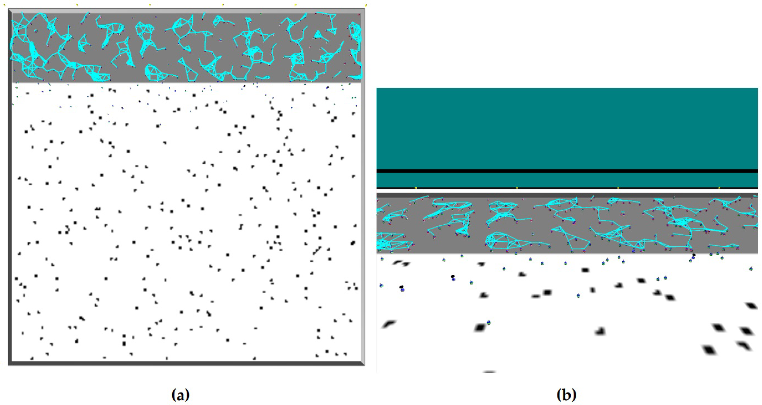
We designed and implemented a set of physics-based simulations using the state-of-the-art simulator for large-scale swarms, ARGoS [15]. An overview of all parameter values used in our simulations is given in

Table 4. Robot and arena parameters used for the simulation setup.

Parameter	Value
Robot parameters
Type	Footbot
Proximity sensor range rprox	0.1 m
Range-and-bearing sensor range rrab	1.25 m
Maximum moving speed	1 $\frac{m}{s}$
No-turn threshold αnt	10°
Soft-turn threshold αst	30°
Hard-turn threshold αht	90°
$s_e,i_e,i_r,s_r\in \left\{0.0,0.01,0.5,0.9\right\}$
Arena parameters
Total area A	50 × 50 m2
Nest area An	10 × 50 m2
Foraging area Af	40 × 50 m2
Number of robots Nrobots	950
Number of items Nitems	300
Radius of an item ritem	0.2 m
Total experiment duration T	104 ts

. The simulations are conducted in a square-shaped arena, which is confined within four walls, each being of the length of 50 m. The arena is divided into two regions: (i) the nest $A_n$: it is the gray $10\times 50$ m² area in Figure 1a, and (ii) the foraging area $A_f$: it is the white $40\times 50$ m² area in Figure 1a. The items are scattered uniformly over the foraging area, and keep reappearing after robots retrieve them to the nest—as in [14]—with constant probability. This prevents the system from drifting into an absorbing state in which there are no items left to recover.

A phototaxis behavior is used to assist the robots in leaving and re-visiting the nest. For that purpose, light beacons are positioned equidistantly at the nest wall (yellow dots at the bottom of Figure 1a). Their light is perceived by the robots’ light sensors. Each robot is programmed to move away from the beacons when it needs to leave the nest and towards the beacons when it needs to return. We use a homogeneous swarm of Footbots (see http://www.swarmanoid.org/swarmanoid_hardware.php) in our simulations, and the communication radius of the robots is set such that the fraction of the circular communication area around the robot is 0.982% of the nest area, which is close to the fraction used in [14]. For better readability, we will limit our discussion of the robot states to only resting and exploring. While the former is distinct, the latter is composed of further states of which only foraging and homing are relevant because they are the most time consuming (for a detailed list of the robot states please see Supplementary Material Section 2).

At the beginning of the simulation, each robot switches from resting to exploring with a probability of 0.01. Consequently, within the first 500 time steps (ts) most robots leave the nest. After another ≈ 500 ts most of the swarm returns, with or without an item. Although this behavior is subsequently repeated several times, the number of simultaneously switching robots gradually decreases, and the switching rate from resting to exploring (or vice versa) approaches a constant limit. In most cases, the system approached an equilibrium after 5 · 10³ ts (for the given arena, item density, and swarm size). Our measurements of the system features begin from that time instance on-wards and the experiment proceeds for another $T={10}^4$ ts.

Furthermore, to conduct a solid statistical study we use large-scale swarms with $N_{robots}=950$ units which is up to an order of magnitude higher than what is commonly used [14,16,36,42]. We selected the value of $N_{robots}$ by running preliminary experiments, in which we observed for this particular swarm size—under the given arena and item density—a maximum in swarm performance.

Finally, in our experiments, the most important means of influencing the swarm dynamics is by adjusting the numerical values of the internal and social cues—$i_e,i_r$ and $s_e,s_r$, respectively—at the start of each experiment. We consider a spectrum of 256 distinct scenario configurations, which differ by the 4-tuples $a=\left(s_e,i_e,i_r,s_r\right)$ drawn from:

$$\Omega :=\{a:s_e,i_e,i_r,s_r\in \{0.0,0.01,0.5,0.9\}\}.$$

(14)

The rationale behind the choice of these parameter values is to include four fundamentally different kinds of cue impact on swarm dynamics: (i) none (ii) low (iii) intermediate and (iv) high. Please note that any additional value in the set a greatly increases the associated computational and analytic effort—as the number of scenarios scales with $dim{\left(a\right)}^4$. However, based on preliminary results, additional values would offer potentially little informative gain (at the current stage) because the swarm dynamics would be similar to a mix of the dynamics generated by the above values.

3. Results and Discussion

We performed simulations with all combinations of cues and communication modes. Each simulation was repeated with 30 random seeds and the data analysis procedure was carried out as discussed in the previous section.

3.1. Presence of Power Law Distributed Features

The analysis of our simulation data shows that in most scenarios there was only weak or no statistical support for the (truncated) power law distribution (see Figure 2A). In particular, in roughly half of all scenarios no power distributed features were found. This observation suggests that in the present system, scale-free features are rare. Nevertheless, we found 245 + 71 = 316 (truncated) power law distributions with moderate or strong statistical plausibility for different features in various scenario configurations and for both communication modes, DCM and CCM. Thus, our findings are in line with a recent study showing that scale-free networks may occur rarely but across different areas [55].

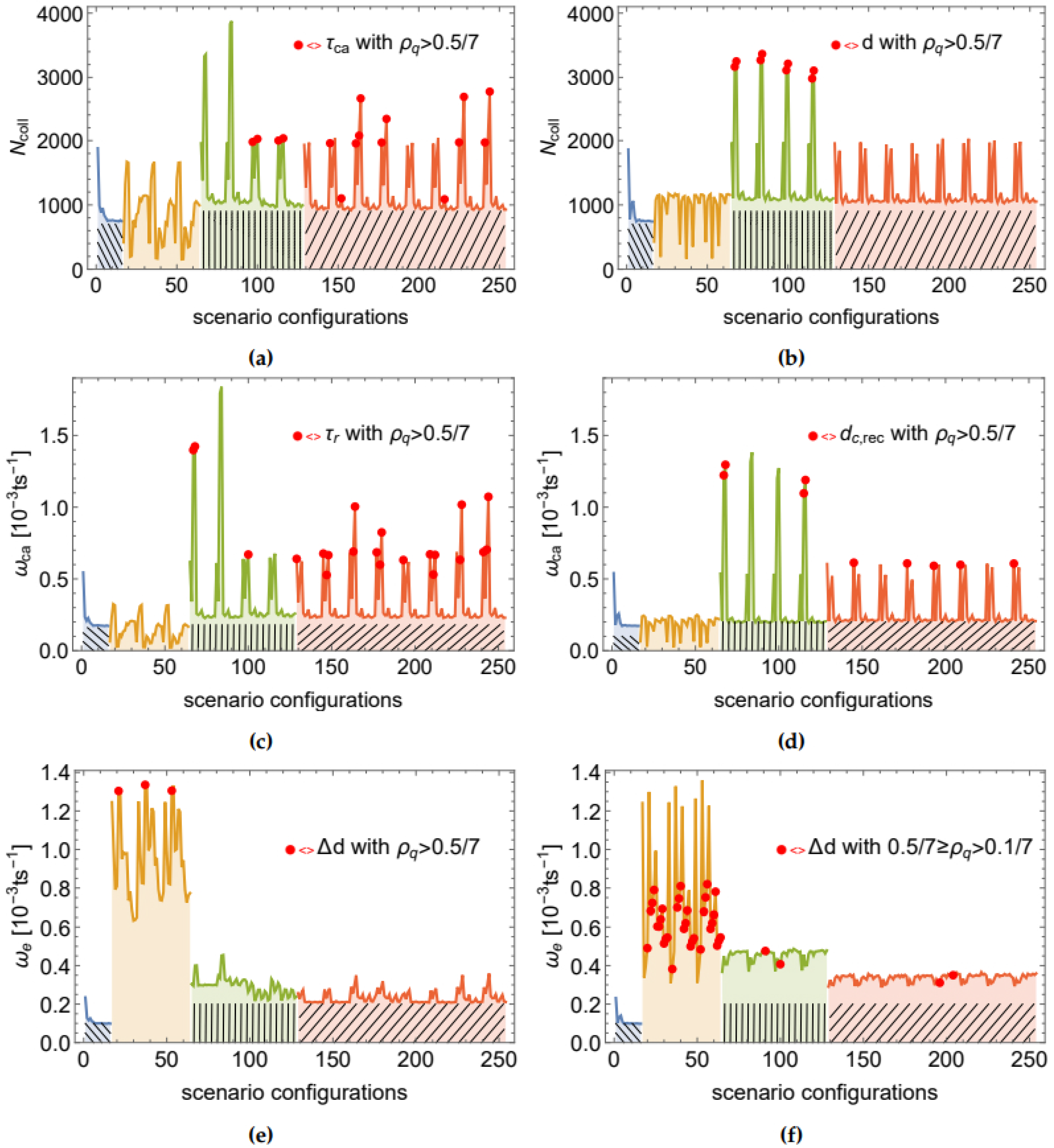
As the scatter plots in Figure 2 show, most of the distributions with weak or moderate support for power law are concentrated below or close to the average values of swarm performance while the distributions with strong support for power law are associated with above-average performance in terms of $N_{coll}$ and ${\omega }_{ca}$. Swarm performance was measured using (i) the number of items retrieved by the robots, $N_{coll}$, (ii) the average number of collected items per time spent on collision avoidance ${\omega }_{ca}$, and (iii) the average number of collected items per time spent exploring ${\omega }_e$. Figure 3 shows the values recorded for these three metrics under both continuous and DCMs and for the entire range of 256 scenario (cues) configurations, respectively. Repeating performance patterns can be observed over different sets of configurations. The regions over which these patterns emerge are (from left to right): (i) all scenarios with $s_e=0$ and $i_e=0$, i.e., constant $p_{r\to e}$ (blue region with a left tilted mesh in Figure 3), (ii) all scenarios with $s_e=0$ and $i_e>0$, i.e., no social and only internal influence on $p_{r\to e}$. This region is henceforth referred to as $N{S}_e$ (shown in orange, no mesh), (iii) all scenarios with $s_e=0.01$, i.e., low social impact on $p_{r\to e}$ (green region with vertical mesh, henceforth denoted as $L{S}_e$), and (iv) all scenarios with $s_e=0.5$ or $s_e=0.9$, i.e., high social influence on $p_{r\to e}$ (red region with right tilted mesh, henceforth denoted as $H{S}_e$). Please note that in all four regions $p_{e\to r}$ is altered in the same way, i.e., for $s_r$ and $i_r$ all values from $\{0.0,0.01,0.5,0.9\}$ are included. The best swarm performance in terms of $N_{coll}$ and ${\omega }_{ca}$ emerges when the influence of internal cues on the swarm dynamics is negligible compared to social cues, i.e., when $s_e{\sum }_t|{\delta }_{\eta }\left(t\right)|\gg i_e{\sum }_t\left|{\delta }_{\varphi }\left(t\right)\right|$ and $s_r{\sum }_t|{\delta }_{\eta }\left(t\right)|\gg i_r{\sum }_t\left|{\delta }_{\varphi }\left(t\right)\right|$.

The best performance levels in terms of $N_{coll}$ and ${\omega }_{ca}$ were reached over the $L{S}_e$ region. For instance, the maxima of $N_{coll}$ and ${\omega }_{ca}$ correspond to the scenario configurations in which $s_e=0.01$, $i_r=0$ and $s_r\ge 0.5$. For the same configurations, (truncated) power law distributions of space features were found in the CCM (examples shown in Figure 4). Contrary to CCM, in the DCM the robot interactions are interrupted. These interruptions may explain why, in DCM, space features such as communication degree tend to not follow a power law distribution (weak overall support for the presence of a power law behavior). Nevertheless, we found fits with moderate to strong support for (truncated) power law to time features, such as ${\tau }_r$ and ${\tau }_{ca}$, demonstrated in Figure 5. The best power law fits of the DCM correspond to the peaks in swarm performance in terms of $N_{coll}$ and ${\omega }_{ca}$ over the $H{S}_e$ regions.

The third performance measure, i.e., ${\omega }_e$, reached its best values over the $N{S}_e$ region. Its maxima correspond to cases where $s_e=0$ and $s_r=0$. Interestingly, for these scenario configurations we found fits with moderate to strong support for (truncated) power law to the data of Δd, i.e., the change of the average communication degree of the robot (examples shown in Figure 6). This is an interesting finding because it indicates that a communication feature may be power law distributed also in those scenarios in which the swarm tries to minimize the number of foraging robots and maximize the number of resting ones. Moreover, in most Δd distributions with strong or moderate support for the power law, the fit includes only 10–20% of data points. The reason for the relatively low ratio of power law fitted data is that the tail of the distribution is likely to represent by the fraction of robots that rest or move close to the border between the nest and the foraging area.

In general, the findings suggest that internal cues (in the absence of social cues) keep robots at the edge of minimal activity while social cues (in the absence of internal cues) drive the robots towards maximal activity.

3.2. Correlation with Swarm Performance

In the previous section we have illustrated that swarm performance is likely to reach its peaks over cue configurations that include asymptotically scale-free space or time features (see Figure 3). In this section, we analyze this observation statistically, using correlation measures such as the Pearson and Kendall’s tau rank correlation coefficients introduced in Section 2.4.3. However, note that both correlation measures have strengths and shortcomings. On the one hand, while the Pearson correlation coefficient is widely used and has an elegant mathematical form, it is sensible to outliers and may not be appropriate for non-linear distributions. On the other hand, Kendall’s tau is suitable for non-linear distributions as well as robust to outliers. Nevertheless, reducing the values to ranks may disregard the significance of the variable’s value being far from the average. In particular, replacing the real value of the quality ratio ${\rho }_q$ by its rank leads to loss of information about the extent to which ${\rho }_q$ represents the quality of the power law distribution. Moreover, following the definition of Kendall’s tau in Equations (11)–(15), each difference between data point pairs is assigned the same weight which may not always be appropriate. For instance, consider the ranked swarm performance in terms of $N_{coll}$ and the corresponding distribution of ${\rho }_q$ in CCM for d in Figure 7a and for $d_{c,sent}$ in Figure 7b, respectively. In both cases, Kendall’s tau defined by Equations (11)–(15) returns values indicating no correlation (i.e., ${\tau }_{Kendall}=0.02$ and ${\tau }_{Kendall}=-0.04$, respectively). However, as evident in Figure 7, both cases show different dynamics, with ${\rho }_q$ for d following $N_{coll}$ more closely than for $d_{c,sent}$. The main reason is that the dominant fluctuations of ${\rho }_q$ close to zero are assigned the same weight (i.e., rank step 1) as the more permanent increase of ${\rho }_q$ for high values of $N_{coll}$. Similar considerations hold for the other features and the DCM. To account for this type of behavior, we use a generalization of Equation (15) that weights the ranking steps by a parameter $\kappa$, which is relative to the average change, such that:

$$\begin{array}{c}\hfill \begin{array}{cc}\hfill {\delta }_{i,j}^{\left(c\right)}& =\left\{\begin{array}{cc}\kappa ,\hfill & \mathrm{if}sgn(x_i-x_j)sgn(y_i-y_j)>0\hfill \\ 0,\hfill & \mathrm{else}\hfill \end{array}\right.\hfill \\ \hfill {\delta }_{i,j}^{\left(x\right)}& =\left\{\begin{array}{cc}\kappa ,\hfill & \mathrm{if}{x}_i=x_j\hfill \\ 0,\hfill & \mathrm{else}\hfill \end{array}\right.\hfill \end{array}\end{array}$$

(15)

and similarly, for ${\delta }_{i,j}^{\left(d\right)}$ and ${\delta }_{i,j}^{\left(y\right)}$. The weight parameter $\kappa$ is given by

$$\kappa =\frac{1}{2}\left(\frac{|x_i-x_j|}{{\mu }_x}+\frac{|y_i-y_j|}{{\mu }_y}\right),$$

(16)

where ${\mu }_x$ and ${\mu }_y$ are averages over all $|x_i-x_j|$ and $|y_i-y_j|$, respectively. For each $i,j$ pair, Equation (16) considers the data distances of both distributions, normalized by their respective mean distances. Consequently, $\kappa$ does not favor any distribution and weights each ranking step relative to other distances. Please note that in general, there is no correlation metric that is perfectly adequate for all types of studies and data distributions; it is thus common to consider appropriate modifications [67,68,69,70]. In the present case, for $\kappa =1$ we obtain the standard Kendall’s tau rank correlation coefficient described in Section 2.4.3. However, by implementing Equation (16), the correlation coefficient is less sensitive to fluctuations than the standard Kendall’s tau, while still being more robust to outliers and non-linearity than the Pearson correlation measure. Therefore, in the following we will use this modified Kendall’s tau rank correlation coefficient to investigate the presence of correlations between ${\rho }_q$ and swarm performance.

The correlations are shown for all features in

Table 5. Correlation coefficients quantifying correlations of ρ_q with N_coll, ω_ca or ω_e.

Property	Correlation with Ncoll	Correlation with ωca	Correlation with ωe
Discontinuous communication mode (DCM)
d	0.11	0.17	−0.03
Δd	−0.19	−0.33	0.64
dc,sent	0.03	−0.05	−0.03
dc,rec	0.14	0.29	−0.51
τca	0.76	0.80	0.06
τr	0.74	0.77	0.08
τf	0.27	0.26	−0.20
τh	0.22	0.28	−0.44
all	0.40	0.42	0.02
Continuous communication mode (CCM)
d	0.50	0.56	0.10
Δd	−0.02	−0.16	0.51
dc,sent	−0.15	−0.39	0.54
dc,rec	0.44	0.44	0.15
τca	0.75	0.80	−0.13
τr	0.59	0.67	−0.02
τf	0.26	0.29	−0.24
τh	0.11	0.17	−0.27
all	0.40	0.41	0.05

A high correlation coefficient means: the better the quality of (truncated) power law distribution, the higher the likelihood that the swarm performed well. Cells highlighted in blue show moderate or strong correlations.

between the three measures of the swarm performance and the feature ’scale-freeness’ quantified by ${\rho }_q$. We found strong correlations of the scale-free property of various features with the swarm performance. In particular, high correlations exist for ${\tau }_{ca},{\tau }_r$, Δd in DCM; and, additionally, for $d,d_{c,rec}$ in CCM. Remarkably, for those features for which we found moderate or high correlation values (highlighted in blue in Table 5), most high-quality power law fits appear in the same scenarios as the highest swarm performance peaks. The red dots in Figure 3 illustrate this finding by highlighting the scenarios in which the quality ratio is ${\rho }_q>\frac{0.5}{7}$. Moreover, the swarm tends to demonstrate low performance with respect to $N_{coll}$ and ${\omega }_{ca}$ for those scenarios in which ${\omega }_e$ is highest, the latter being well correlated with Δd.

The correlation coefficients confirm the observation, supported by the data shown in Figure 2 and Figure 3, that most power law distributions with strong support (i.e., high ${\rho }_q$) appear in scenarios with peak swarm performance. To further examine this observation, we consider the correlations of the swarm performance with different ${\rho }_q$ support classifications (based on Table 3). As

Table 6. Correlation coefficients between ρ_q and N_coll, ω_ca or ω_e for different power law support classifications.

Support for pl	Correlation with Ncoll	Correlation with ωca	Correlation with ωe
Discontinuous communication mode (DCM)
weak	0.18	0.18	−0.16
moderate	0.10	0.08	0.21
strong	0.31	0.40	−0.14
moderate + strong	0.50	0.53	0.22
Continuous communication mode (CCM)
weak	0.10	0.11	0.03
moderate	0.37	0.33	0.03
strong	0.66	0.63	−0.25
moderate + strong	0.74	0.76	−0.02

Correlation of the swarm performance with different categories of power law distribution support. Cells highlighted in blue show moderate or strong correlation values.

shows, there are moderate and strong positive correlations between features with strong support for power law distribution and swarm performance in terms of $N_{coll}$ and ${\omega }_{ca}$ for both communication modes. This suggests that the observation of scale-free features is more likely in scenarios in which the agents are more successful in retrieving a high number of food items.

3.3. The Role of Feedback Mechanisms in the Emergence of Scale-Free Features

An attribute of complex systems that is widely known to support the emergence of scale-free characteristics is the presence of (positive and negative) feedback loops [1,53,71]. We specify the feedback effect to be positive or negative based on the individual response to the information input from its neighborhood. Hence, we refer to the feedback mechanism as positive feedback if it pushes the individuals to the same state as the state of the majority, whereas negative feedback pushes them away from it.

Most scale-free features were found in scenarios in which (i) the robot behavior was dominated by social interactions, (ii) the swarm attempted to balance positive and negative feedback and (iii) the swarm displayed a tendency towards active exploration. In particular, in CCM, the first 17 scenarios sorted by ${\rho }_q$ in descending order were found over the $L{S}_e$ region and with $i_r=0$. Similarly, in DCM, the first 28 scenarios were found over the $H{S}_e$ region and with $i_r=0$. To understand this, it is necessary to consider in more detail the impact of each cue on swarm dynamics and the feedback mechanisms.

For conciseness, we focus our system analysis on CCM and its most relevant set of parameter configurations. Similar conclusions hold for DCM. In particular, we can simplify our analysis based on the repeating patterns of swarm performance (see Figure 3) and the following observations: (i) The swarm performance is qualitatively very similar between the cue values 0.5 and 0.9 (for all four cues). Thus, we focus, in the following, on $\{a:s_e,i_e,i_r,s_r\in \{0.0,0.01,0.5\}\}$. (ii) The cue $i_e$ has a negligible impact on the foraging dynamics when $s_e>0$. By neglecting scenarios in which $i_e\ne 0$, except those with $s_e=0$, we can further shorten the set of relevant scenarios. Finally, (iii) there are significant differences in the dynamics between scenario configurations with $i_r=0$ and those with $i_r>0$ but negligible differences between $i_r=0.01$ and $i_r=0.5,0.9$. Thus, we focus, in the following, only on scenarios with either $i_r=0$ or $i_r=0.01$. Figure 8 shows the final set of 24 scenarios relevant to the discussion below.

Please note that (ii) and (iii) are consequences of the internal cues $i_e$ and $i_r$ acting only on exploring robots. In the exploring state, the crucial parameter is $p_{e\to r}$ because it defines the probability to stop exploring and change to resting. A non-zero value of the internal cue $i_r$ has a substantial impact on dynamics as it alters $p_{e\to r}$ after each exploration attempt. As the likelihood of finding and retrieving a food item is low, $i_r$ mostly reduces $p_{e\to r}$. The more $p_{e\to r}$ is lowered by $i_r$, the less likely the robot is to find a food item during the next exploration attempt. Thus, $i_r$ has a strong inhibitory influence on the swarm’s exploration activity. Consequently, there is a significant difference in swarm performance between the scenario configurations with $i_r=0$ and those with $i_r>0$. As the swarm actively attempts to explore the environment and collect food items, the influence of $i_r>0$ can be considered an important driver of negative feedback. In contrast, $p_{r\to e}$ acts only on resting robots. Consequently, any change of $p_{r\to e}$ through $i_e$ is easily distorted by $s_e$, i.e., the social interactions with the neighborhood of the resting robot. Hence, only when $s_e=0$ there is an inhibitory impact of $i_e$ on swarm dynamics (similar to $i_r$, due to the scarcity of food items), otherwise $i_e$ is negligible. In short, when the probability of finding a food item is low, with $i_r=0$ and $s_e>0$ enabling the swarm to significantly damp the feedback mechanisms that drive the swarm towards inactivity.

Next, we consider the particular contributions of social cues $s_e$ and $s_r$. Social interactions represent a direct form of feedback loops, enabling the swarm to drift towards an absorbing state (e.g., uninterrupted resting or exploring) or maintain a balance between positive and negative feedback. In general, note that high values of $s_e$ often lead to $p_{r\to e}=0$ due to the high probability of encountering a robot with a failed exploration (due to the low density of food items). With such relatively high values of $s_e$, $p_{r\to e}$ can be reduced to zero within a few time steps. By contrast, with $s_e=0.01$, $p_{r\to e}$ does not fluctuate as strongly. Similar considerations hold for $s_r$ and $p_{e\to r}$. In terms of active exploration, i.e., long exploration times and high number of retrieved items, it is beneficial for the swarm to have robots with $p_{r\to e}=1$ and $p_{e\to r}=0$. Indeed, in the present system we observe that the swarm approaches such behavior for $s_r=0.5$ and $s_e=0.01$ (i.e., over the $L{S}_e$ region). More importantly, such balance of $s_r$ and $s_e$ allows positive and negative feedback loops to coexist with the positive feedback being slightly more dominant. Due to this feedback coexistence, a robot that happened to be surrounded by unsuccessful neighbors will tend to have low $p_{r\to e}$ and high $p_{e\to r}$, i.e., its resting time ${\tau }_r$ will increase (together with its d or $d_{c,rec}$) and vice versa. Over time, such dynamics will result in robots that are increasingly inactive (with increasingly higher ${\tau }_r$, d or $d_{c,rec}$) and robots that are increasingly active (with increasingly lower ${\tau }_r$, d or $d_{c,rec}$). When the majority tends towards active exploration, the inactive group of robots experiences negative feedback and while the active group is subject to positive feedback. The prevalence of the positive feedback decreases the number of consistently resting robots significantly below the number of consistently exploring ones. Ultimately, this leads to skewed or heavy tailed distributions, such as the power law and, consequently, to the emergence of scale-free features. Similar considerations apply to the DCM over the $H{S}_e$ region. The difference is that in DCM each robot can broadcast its exploration result only once. Thus, $s_e$ needs to have high values for dynamics similar to CCM to emerge.

To illustrate the above considerations, let us examine the scenario configuration of CCM with $s_e=0.01$, $i_e=0.9$, $i_r=0.0$, and $s_r=0.5$ (see Figure 4a), in which a high performance value of $N_{coll}$ was observed (i.e., this scenario is similar to the peak in Figure 8). The value of $s_r$ has a high impact on $p_{e\to r}$ (the probability to transition to resting). For example, if a robot receives at least two ‘success’ messages more than ‘failure’ messages—i.e., if ${\delta }_{\eta }\left(t_r\right)\ge 2$ in Equation (2)—its $p_{e\to r}$ drops to zero. When $p_{e\to r}=0$ and $i_r=0.0$, the robot will stop exploring only if it finds an item. During the subsequent resting, this robot is likely to cause one of its neighbors to reach $p_{e\to r}=0$, which repeats an analogous cycle of events. The corresponding dynamics can be translated in terms of the positive feedback pushing the robots out of the nest and increasing the number of robots in the foraging area (i.e., in the exploring state). In the long term, due to the positive feedback, the swarm drifts towards the absorbing state in which all robots have $p_{e\to r}=0$ and $p_{r\to e}=1.0$. In the short term, while most robots is exploring, some robots remain in the nest, e.g., due to crowding at the entrance of the nest. Those robots have a higher number of neighbors because the nest is significantly smaller than the foraging area. Therefore, during this crowding behavior, the swarm experiences the coexistence of positive and negative feedback loops. A specific balance between these feedback loops may lead to the emergence of scale-free features such as the space feature d (for which, indeed, the above mentioned scenario configuration has one of the best truncated power law fits with ${\rho }_q\approx 0.23$, shown in Figure 4a). Similar considerations hold for other CCM examples presented in Figure 4 or the DCM examples in Figure 5.

The above example demonstrates positive feedback regarding the exploring state. However, under some configurations, positive feedback can also be observed around the resting state. For example, during the crowding behavior in the nest, a robot which is surrounded by a high number of resting neighbors is likely to get ‘stuck’ and be unable to leave the nest. This robot will eventually switch to the resting state and broadcast a ‘failure’ message. Neighbors that receive this message will decrease their probability to explore $p_{r\to e}$, and, through physical interference, lower the neighboring robots’ chances to leave the nest. Consequently, positive feedback at the resting state may lead, in the long term, to an increase of the average communication degree of the resting robots and the emergence of power law distributed features, alongside the occurrence of outstanding robots whose features such as Δd (examples shown in Figure 6), ${\tau }_r$ or ${\tau }_{ca}$ exhibit exceptionally above-average values.

4. Conclusions

In this paper, we have investigated the interplay between scale-free features and swarm dynamics of a foraging swarm. Our results demonstrate that in the studied system (i) several space and time features tend to be asymptotically scale-free for multiple parameter configurations; (ii) the emergence of scale-free features can be attributed to the presence of positive/negative feedback mechanisms. Furthermore, (iii) in several cases the swarm performance is moderately or strongly correlated with the tendency of space and time features to follow the power law distribution—which is the mathematical backbone of the scale-free property.

This study serves as a first step towards a better understanding of the interplay between the presence of scale-free features and the swarm behavior in terms of collective performance. Although our results do not indicate a causal relationship, we found conclusive evidence for a close connection between scale-free features and swarm performance. Moreover, our analysis of power law distributed features shows a strong link between the microscopic behavior of robots determined by specific cues and the macroscopic behavior of the entire swarm exhibiting peak performance. However, care needs to be taken when considering cases where the power law fit includes only a small fraction of data, as focusing on a small subgroup that plausibly displays scale-free features may disregard a significant piece of information about the global swarm behavior.

Please note that the presented exploratory study was conducted with an emphasis on whether scale-free features may emerge autonomously in artificial multi-agent systems, without focusing on why they do so. Hence, more sophisticated work is needed to precisely understand the exact causes for the emergent scale-free characteristics in our systems. For instance, strong feedback mechanisms may push the system close to a critical point at which a phase-transition occurs. In case of a continuous phase-transition, the latter is known to be associated with the emergence of scale-free features [1,53]. In fact, using approximations (such as the assumption of a well-mixed system) it could be shown analytically that the social or internal cues can be used as control parameters, moving the system between its phases (e.g., phases in which the number of resting robots is minimized or maximized). However, if the system approaching a phase-transition is the cause for the emergence of scale-free features in our experiments, we expect to find a correlation length (i.e., the distance over which one robot influences another, directly or indirectly) that is longer than the size of the system (e.g., the length of the nest). In contrast, our preliminary analysis indicated the opposite behavior: as we approached those scenarios in which scale-free characteristics were observed, the correlation length decreased below the system size. In general, a detailed finite-size-scaling analysis is necessary to explain our findings more thoroughly as well as reveal which (physical) boundaries are most relevant and what impact they have on the system dynamics.

The canonical foraging task continues drawing scientific attention due its importance and prevalence in nature as well as artificial systems. In addition, the complexity of collective foraging as a combination of several sub-behaviors allows the modeling and analysis of a large number of scenarios and examine various features. For these reasons, we focused exclusively on the foraging behavior. However, it would be interesting to extend the scope and investigate other multi-agent tasks, such as aggregation or flocking, from the same perspective as in our study thereby broadening the understanding of scale-free phenomena in artificial collective systems.

References

- Khaluf, Y.; Ferrante, E.; Simoens, P.; Huepe, C. Scale invariance in natural and artificial collective systems: A review. J. R. Soc. Interface 2017, 14, 20170662. [Google Scholar] [CrossRef] [PubMed]
- Cavagna, A.; Cimarelli, A.; Giardina, I.; Parisi, G.; Santagati, R.; Stefanini, F.; Viale, M. Scale-free correlations in starling flocks. Proc. Natl. Acad. Sci. USA 2010, 107, 11865–11870. [Google Scholar] [CrossRef] [PubMed] [Green Version]
- Huepe, C.; Ferrante, E.; Wenseleers, T.; Turgut, A.E. Scale-Free Correlations in Flocking Systems with Position-Based Interactions. J. Stat. Phys. 2015, 158, 549–562. [Google Scholar] [CrossRef]
- Chen, X.; Dong, X.; Be’er, A.; Swinney, H.L.; Zhang, H.P. Scale-Invariant Correlations in Dynamic Bacterial Clusters. Phys. Rev. Lett. 2012, 108, 148101. [Google Scholar] [CrossRef] [PubMed]
- Boyer, D.; Ramos-Fernández, G.; Miramontes, O.; Mateos, J.L.; Cocho, G.; Larralde, H.; Ramos, H.; Rojas, F. Scale-free foraging by primates emerges from their interaction with a complex environment. Proc. R. Soc. B Biol. Sci. 2006, 273, 1743–1750. [Google Scholar] [CrossRef] [PubMed] [Green Version]
- Reynolds, A.M.; Ouellette, N.T. Swarm dynamics may give rise to Lévy flights. Sci. Rep. 2016, 6, 30515. [Google Scholar] [CrossRef] [PubMed]
- Albert, R.; Barabási, A.L. Statistical mechanics of complex networks. Rev. Mod. Phys. 2002, 74, 47–97. [Google Scholar] [CrossRef] [Green Version]
- Fewell, J.H. Social Insect Networks. Science 2003, 301, 1867–1870. [Google Scholar] [CrossRef]
- Kasthurirathna, D.; Piraveenan, M. Emergence of scale-free characteristics in socio-ecological systems with bounded rationality. Sci. Rep. 2015, 5, 10448. [Google Scholar] [CrossRef]
- Goh, K.I.; Kahng, B.; Kim, D. Universal Behavior of Load Distribution in Scale-Free Networks. Phys. Rev. Lett. 2001, 87, 278701. [Google Scholar] [CrossRef] [Green Version]
- Cohen, R.; Havlin, S. Scale-Free Networks Are Ultrasmall. Phys. Rev. Lett. 2003, 90, 058701. [Google Scholar] [CrossRef] [PubMed] [Green Version]
- Thivierge, J.P. Scale-free and economical features of functional connectivity in neuronal networks. Phys. Rev. E 2014, 90, 022721. [Google Scholar] [CrossRef] [PubMed]
- Albert, R.; Jeong, H.; Barabási, A.L. Error and attack tolerance of complex networks. Nature 2000, 406, 378–382. [Google Scholar] [CrossRef] [PubMed] [Green Version]
- Liu, W.; Winfield, A.F.T.; Sa, J.; Chen, J.; Dou, L. Towards Energy Optimization: Emergent Task Allocation in a Swarm of Foraging Robots. Adapt. Behav. 2007, 15, 289–305. [Google Scholar] [CrossRef]
- Pinciroli, C.; Trianni, V.; O’Grady, R.; Pini, G.; Brutschy, A.; Brambilla, M.; Mathews, N.; Ferrante, E.; Di Caro, G.; Ducatelle, F.; et al. ARGoS: A modular, parallel, multi-engine simulator for multi-robot systems. Swarm Intell. 2012, 6, 271–295. [Google Scholar] [CrossRef]
- Pini, G.; Brutschy, A.; Pinciroli, C.; Dorigo, M.; Birattari, M. Autonomous task partitioning in robot foraging: An approach based on cost estimation. Adapt. Behav. 2013, 21, 118–136. [Google Scholar] [CrossRef]
- Brambilla, M.; Ferrante, E.; Birattari, M.; Dorigo, M. Swarm robotics: A review from the swarm engineering perspective. Swarm Intell. 2013, 7, 1–41. [Google Scholar] [CrossRef]
- Bayındır, L. A Review of Swarm Robotics Tasks. Neurocomput. 2016, 172, 292–321. [Google Scholar] [CrossRef]
- Khaluf, Y.; Dorigo, M. Modeling robot swarms using integrals of birth-death processes. ACM Trans. Auton. Adapt. Syst. (TAAS) 2016, 11, 8. [Google Scholar] [CrossRef]
- Khaluf, Y.; Pinciroli, C.; Valentini, G.; Hamann, H. The impact of agent density on scalability in collective systems: Noise-induced versus majority-based bistability. Swarm Intell. 2017, 11, 155–179. [Google Scholar] [CrossRef]
- Yang, G.Z.; Bellingham, J.; Dupont, P.E.; Fischer, P.; Floridi, L.; Full, R.; Jacobstein, N.; Kumar, V.; McNutt, M.; Merrifield, R.; et al. The grand challenges of Science Robotics. Sci. Robot. 2018, 3. [Google Scholar] [CrossRef]
- Ferrante, E.; Turgut, A.E.; Huepe, C.; Stranieri, A.; Pinciroli, C.; Dorigo, M. Self-organized flocking with a mobile robot swarm: A novel motion control method. Adapt. Behav. 2012, 20, 460–477. [Google Scholar] [CrossRef]
- Khaluf, Y.; Rausch, I.; Simoens, P. The Impact of Interaction Models on the Coherence of Collective Decision-Making: A Case Study with Simulated Locusts. In Swarm Intelligence; Dorigo, M., Birattari, M., Blum, C., Christensen, A.L., Reina, A., Trianni, V., Eds.; Springer International Publishing: Cham, Switzerland, 2018; pp. 252–263. [Google Scholar] [Green Version]
- Correll, N.; Martinoli, A. Modeling and designing self-organized aggregation in a swarm of miniature robots. Int. J. Robot. Res. 2011, 30, 615–626. [Google Scholar] [CrossRef]
- Deneubourg, J.L.; Goss, S. Collective patterns and decision-making. Ethol. Ecol. Evol. 1989, 1, 295–311. [Google Scholar] [CrossRef]
- Sumpter, D.J. The principles of collective animal behaviour. Philos. Trans. R. Soc. B Biol. Sci. 2005, 361, 5–22. [Google Scholar] [CrossRef] [PubMed]
- Batalin, M.A.; Sukhatme, G.S. Spreading Out: A Local Approach to Multi-robot Coverage. In Distributed Autonomous Robotic Systems 5; Asama, H., Arai, T., Fukuda, T., Hasegawa, T., Eds.; Springer: Tokyo, Japan, 2002; pp. 373–382. [Google Scholar] [Green Version]
- Ren, H.; Tse, Z.T.H. Investigation of Optimal Deployment Problem in Three-Dimensional Space Coverage for Swarm Robotic System. In Social Robotics; Ge, S.S., Khatib, O., Cabibihan, J.J., Simmons, R., Williams, M.A., Eds.; Springer: Berlin/Heidelberg, Germany, 2012; pp. 468–474. [Google Scholar]
- Mclurkin, J.; Smith, J. Distributed algorithms for dispersion in indoor environments using a swarm of autonomous mobile robots. In Distributed Autonomous Robotic Systems 6; Asama, H., Alami, R., Chatila, R., Eds.; Springer: Tokyo, Japan, 2007; pp. 399–408. [Google Scholar]
- Sharma, S.; Shukla, A.; Tiwari, R. Multi robot area exploration using nature inspired algorithm. Biol. Inspired Cogn. Archit. 2016, 18, 80–94. [Google Scholar] [CrossRef]
- Schmickl, T.; Crailsheim, K. A Navigation Algorithm for Swarm Robotics Inspired by Slime Mold Aggregation. In Swarm Robotics; Şahin, E., Spears, W.M., Winfield, A.F.T., Eds.; Springer: Berlin/Heidelberg, Germany, 2007; pp. 1–13. [Google Scholar]
- Gauci, M.; Chen, J.; Dodd, T.J.; Groß, R. Evolving Aggregation Behaviors in Multi-Robot Systems with Binary Sensors. In Distributed Autonomous Robotic Systems; Ani Hsieh, M., Chirikjian, G., Eds.; Springer: Berlin/Heidelberg, Germnay, 2014; pp. 355–367. [Google Scholar] [Green Version]
- Pitonakova, L.; Crowder, R.; Bullock, S. Information flow principles for plasticity in foraging robot swarms. Swarm Intell. 2016, 10, 33–63. [Google Scholar] [CrossRef] [Green Version]
- Bullock, S.; Crowder, R.; Pitonakova, L. Task Allocation in Foraging Robot Swarms: The Role of Information Sharing. In Proceedings of the The 2018 Conference on Artificial Life: A Hybrid of the European Conference on Artificial Life (ECAL) and the International Conference on the Synthesis and Simulation of Living Systems (ALIFE), Cancun, Mexico, 4–8 July 2016; pp. 306–313. [Google Scholar]
- Ostergaard, E.H.; Sukhatme, G.S.; Matari, M.J. Emergent bucket brigading: A simple mechanisms for improving performance in multi-robot constrained-space foraging tasks. In Proceedings of the Fifth International Conference on Autonomous Agents, Montreal, QC, Canada, 28 May–1 June 2001; pp. 29–30. [Google Scholar]
- Hamann, H.; Wörn, H. An Analytical and Spatial Model of Foraging in a Swarm of Robots. In Swarm Robotics: Second International Workshop, SAB 2006, Rome, Italy, September 30–October 1, 2006, Revised Selected Papers; Şahin, E., Spears, W.M., Winfield, A.F.T., Eds.; Springer: Berlin/Heidelberg, Germany, 2007; pp. 43–55. [Google Scholar] [Green Version]
- Hoff, N.R.; Sagoff, A.; Wood, R.J.; Nagpal, R. Two foraging algorithms for robot swarms using only local communication. In Proceedings of the 2010 IEEE International Conference on Robotics and Biomimetics, Tianjin, China, 14–18 December 2010; pp. 123–130. [Google Scholar]
- Hecker, J.P.; Letendre, K.; Stolleis, K.; Washington, D.; Moses, M.E. Formica ex Machina: Ant Swarm Foraging from Physical to Virtual and Back Again. In Swarm Intelligence; Dorigo, M., Birattari, M., Blum, C., Christensen, A.L., Engelbrecht, A.P., Groß, R., Stützle, T., Eds.; Springer: Berlin/Heidelberg, Germany, 2012; pp. 252–259. [Google Scholar]
- Castañeda Cisneros, J.; Pomares Hernandez, S.E.; Perez Cruz, J.R.; Rodríguez-Henríquez, L.M.; Gonzalez Bernal, J.A. Data-Foraging-Oriented Reconnaissance Based on Bio-Inspired Indirect Communication for Aerial Vehicles. Appl. Sci. 2017, 7, 729. [Google Scholar] [CrossRef]
- Wang, H.; Li, Y.; Chang, T.; Chang, S.; Fan, Y. Event-Driven Sensor Deployment in an Underwater Environment Using a Distributed Hybrid Fish Swarm Optimization Algorithm. Appl. Sci. 2018, 8, 1638. [Google Scholar] [CrossRef]
- Hernández-Ocaña, B.; Hernández-Torruco, J.; Chávez-Bosquez, O.; Calva-Yáñez, M.B.; Portilla-Flores, E.A. Bacterial Foraging-Based Algorithm for Optimizing the Power Generation of an Isolated Microgrid. Appl. Sci. 2019, 9, 1261. [Google Scholar] [CrossRef]
- Lerman, K.; Galstyan, A. Mathematical Model of Foraging in a Group of Robots: Effect of Interference. Auton. Robot. 2002, 13, 127–141. [Google Scholar] [CrossRef]
- Khaluf, Y.; Birattari, M.; Rammig, F. Analysis of long-term swarm performance based on short-term experiments. Soft Comput. 2016, 20, 37–48. [Google Scholar] [CrossRef]
- Hoff, N.; Wood, R.; Nagpal, R. Distributed colony-level algorithm switching for robot swarm foraging. In Distributed Autonomous Robotic Systems; Springer: Berlin/Heidelberg, Germany, 2013; pp. 417–430. [Google Scholar]
- Schafer, R.J.; Holmes, S.; Gordon, D.M. Forager activation and food availability in harvester ants. Anim. Behav. 2006, 71, 815–822. [Google Scholar] [CrossRef]
- Prabhakar, B.; Dektar, K.N.; Gordon, D.M. The Regulation of Ant Colony Foraging Activity without Spatial Information. PLoS Comput. Biol. 2012, 8, 1–7. [Google Scholar] [CrossRef] [PubMed]
- Pinter-Wollman, N.; Bala, A.; Merrell, A.; Queirolo, J.; Stumpe, M.; Holmes, S.; Gordon, D. Harvester ants use interactions to regulate forager activation and availability. Anim. Behav. 2013, 86, 197–207. [Google Scholar] [CrossRef] [Green Version]
- Seeley, T.D.; Visscher, P.K.; Schlegel, T.; Hogan, P.M.; Franks, N.R.; Marshall, J.A.R. Stop Signals Provide Cross Inhibition in Collective Decision-Making by Honeybee Swarms. Science 2012, 335, 108–111. [Google Scholar] [CrossRef] [Green Version]
- Reina, A.; Valentini, G.; Fernández-Oto, C.; Dorigo, M.; Trianni, V. A Design Pattern for Decentralised Decision Making. PLoS ONE 2015, 10, 0140950. [Google Scholar] [CrossRef]
- Valentini, G.; Ferrante, E.; Hamann, H.; Dorigo, M. Collective decision with 100Kilobots: Speed versus accuracy in binary discrimination problems. Auton. Agents Multi-Agent Syst. 2016, 30, 553–580. [Google Scholar] [CrossRef]
- Khaluf, Y.; Birattari, M.; Rammig, F. Probabilistic analysis of long-term swarm performance under spatial interferences. In Proceedings of the International Conference on Theory and Practice of Natural Computing, Cáceres, Spain, 3–5 December 2013; pp. 121–132. [Google Scholar]
- Hamann, H.; Valentini, G.; Khaluf, Y.; Dorigo, M. Derivation of a micro-macro link for collective decision-making systems. In Proceedings of the International Conference on Parallel Problem Solving from Nature; Springer: Cham, Switzerland, 2014; pp. 181–190. [Google Scholar]
- Newman, M.E. Power laws, Pareto distributions and Zipf’s law. Contemp. Phys. 2005, 46, 323–351. [Google Scholar] [CrossRef]
- Clauset, A.; Shalizi, C.R.; Newman, M.E.J. Power-Law Distributions in Empirical Data. SIAM Rev. 2009, 51, 661–703. [Google Scholar] [CrossRef] [Green Version]
- Broido, A.D.; Clauset, A. Scale-free networks are rare. Nat. Commun. 2019, 10, 1017. [Google Scholar] [CrossRef] [PubMed]
- Alstott, J.; Bullmore, E.; Plenz, D. Powerlaw: A Python Package for Analysis of Heavy-Tailed Distributions. PLoS ONE 2014, 9, e85777. [Google Scholar] [CrossRef] [PubMed]
- Viswanathan, G.M.; Afanasyev, V.; Buldyrev, S.; Murphy, E.; Prince, P.; Stanley, H.E. Lévy flight search patterns of wandering albatrosses. Nature 1996, 381, 413–415. [Google Scholar] [CrossRef]
- Galton, F. The Journal of the Anthropological Institute of Great Britain and Ireland; Number v. 15; Anthropological Institute of Great Britain and Ireland: London, UK, 1886. [Google Scholar]
- Pearson, K. Proceedings of the Royal Society of London; Number v. 58; Taylor & Francis: Abingdon, UK, 1895. [Google Scholar]
- Lee Rodgers, J.; Nicewander, W.A. Thirteen ways to look at the correlation coefficient. Am. Stat. 1988, 42, 59–66. [Google Scholar] [CrossRef]
- Kraaikamp, F.D.C.; Meester, H.L.L. A Modern Introduction to Probability and Statistics; Springer: Berlin/Heidelberg, Germany, 2005. [Google Scholar]
- McDonald, J.H. Handbook of Biological Statistics; Sparky House Publishing: Baltimore, MD, USA, 2009; Volume 2. [Google Scholar]
- Wang, Y.; Li, Y.; Cao, H.; Xiong, M.; Shugart, Y.Y.; Jin, L. Efficient test for nonlinear dependence of two continuous variables. BMC Bioinform. 2015, 16, 260. [Google Scholar] [CrossRef] [PubMed]
- Spearman, C. The Proof and Measurement of Association between Two Things. Am. J. Psychol. 1904, 15, 72–101. [Google Scholar] [CrossRef]
- Kendall, M.G. A new measure of rank correlation. Biometrika 1938, 30, 81–93. [Google Scholar] [CrossRef]
- Christensen, D. Fast algorithms for the calculation of Kendall’s τ. Comput. Stat. 2005, 20, 51–62. [Google Scholar] [CrossRef]
- Blest, D.C. Theory & Methods: Rank Correlation—An Alternative Measure. Aust. N. Z. J. Stat. 2000, 42, 101–111. [Google Scholar]
- Darken, P.F.; Holtzman, G.I.; Smith, E.P.; Zipper, C.E. Detecting changes in trends in water quality using modified Kendall’s tau. Environmetrics 2000, 11, 423–434. [Google Scholar] [CrossRef]
- Emond, E.J.; Mason, D.W. A new rank correlation coefficient with application to the consensus ranking problem. J. Multi-Criteria Decis. Anal. 2002, 11, 17–28. [Google Scholar] [CrossRef]
- Sengupta, D.; Maulik, U.; Bandyopadhyay, S. Entropy steered Kendall’s tau measure for a fair Rank Aggregation. In Proceedings of the 2011 2nd National Conference on Emerging Trends and Applications in Computer Science, Shillong, India, 4–5 March 2011; pp. 1–5. [Google Scholar]
- Khaluf, Y.; Hamann, H. On the definition of self-organizing systems: Relevance of positive/negative feedback and fluctuations. In Proceedings of the Swarm Intelligence: 10th International Conference, ANTS 2016, Brussels, Belgium, 7–9 September 2016; Springer: New York, NY, USA, 2016; Volume 9882, p. 298. [Google Scholar]
Figure 1.
Illustrations of the arena. (a) A snapshot from a simulation in ARGoS. Gray area: nest; white area: foraging field; black dots: items; blue objects: Footbots; light-blue lines: communication (range-and-bearing) links. (b) 3D view on the same arena. In both figures, the communication links are formed only for resting robots inside the nest, as in our experiments moving robots neither broadcast nor listen to any messages.
Figure 2.
(a) Feature data sets obtained from simulations, sorted by the type of statistical support for a corresponding power law fit. The classifications follow Table 3. (b–d) Log-linear scatter plots relating the power law fit quality ratio ρq to the swarm performance in terms of Ncoll, ωca and ωe, respectively. The vertical dashed lines indicate the mean performance values while the horizontal dashed lines separate the quality categorizations taken from Table 3.
Figure 3.
Swarm performance in terms of (a,b) Ncoll; (c,d) ωca and (e,f) ωe, respectively. For each performance measure, 256 scenario configurations were implemented (i.e., with all cue values from Equation (14)), using one of two communication modes: DCM (left) and CCM (right). The x-axis represents the IDs of the scenario configurations. The colors and the mesh patterns highlight regions that display different dynamics. Apart from (f), in all plots the red dots mark the scenarios in which the feature mentioned in the inset demonstrated a high value of ρq, i.e., there was a strong support for the distribution to be power law. In (f), the red dots mark the scenarios with moderate support. See Supplementary Material Section 3 for combined plots of Ncoll and d distribution in CCM over the complete set of 256 scenario configurations.
Figure 4.
Log-log scale plots of the degree d (top) and the critical degree dc,rec (bottom) distributions in CCM. The black lines represent the corresponding truncated power law fits. The insets show the fit parameters as well as the scenario configurations. The plots (a) and (b) differ by the scenario configurations shown in the insets; similarly for (c) and (d). These scenarios are among the top five swarm performances with respect to Ncoll. Please note that λxmin is relatively small, i.e., power law is a good fit for x close to xmin. See Supplementary Material Section 3 for plots of d in CCM over all 256 scenario configurations.
Figure 5.
Log-log scale plots of the resting time τr (top) and the collision avoidance time τca (bottom) distributions in DCM. The black lines represent the corresponding truncated power law fits. The insets show the fit parameters as well as the scenario configurations. The plots (a,b) differ by the scenario configurations shown in the insets; similarly for (c,d). These scenarios belong to a subset of the best swarm performance with respect to ωca. Please note that λ = 0 for the fits of τca, indicating better support for the power law fit than for truncated power law.
Figure 6.
Log-log scale plots of Δd per 100 ts in CCM. The black lines represent the corresponding truncated power law fits. The insets show the fit parameters as well as the scenario configurations. The plots (a,b) differ by the scenario configurations shown in the insets. These scenarios are among the best swarm performances with respect to ωe.
Figure 7.
Ranked distribution of Ncoll (dark red, left y-axis). For the same cue configurations, the CCM distributions of ρq (right y-axis) for (a) d and (b) dc,sent are shown in blue, respectively. The insets depict the corresponding scatter plots with data points representing weak (circles), moderate (triangles) and strong (squares) support for power law distribution; gray lines indicate the onsets of the different support classifications (similar to Figure 2).
Figure 8.
Number of collected items for a selected set of 24 scenario configurations a in CCM. The data labels show the corresponding cue values of .