Dual-Channel Speech Enhancement Based on Extended Kalman Filter Relative Transfer Function Estimation ^†

Abstract

This paper deals with speech enhancement in dual-microphone smartphones using beamforming along with postfiltering techniques. The performance of these algorithms relies on a good estimation of the acoustic channel and speech and noise statistics. In this work we present a speech enhancement system that combines the estimation of the relative transfer function (RTF) between microphones using an extended Kalman filter framework with a novel speech presence probability estimator intended to track the noise statistics’ variability. The available dual-channel information is exploited to obtain more reliable estimates of clean speech statistics. Noise reduction is further improved by means of postfiltering techniques that take advantage of the speech presence estimation. Our proposal is evaluated in different reverberant and noisy environments when the smartphone is used in both close-talk and far-talk positions. The experimental results show that our system achieves improvements in terms of noise reduction, low speech distortion and better speech intelligibility compared to other state-of-the-art approaches.

1. Introduction

Speech-related services are pervasively available on mobile devices such as smartphones or tablets. However, reverberant and noisy environments, where these devices are frequently used, often degrade speech signal quality and/or intelligibility [1]. Many current devices include several microphones, so that multi-channel speech processing techniques can be applied to reduce the distortions, which improves the noise reduction performance compared to single-channel approaches. This is our research focus.

The most common multi-channel speech processing technique is beamforming [2], which applies spatial filtering to the noisy speech signals captured by several microphones. One of these beamformers is the well-known Minimum Variance Distortionless Response (MVDR) beamformer [3], which has the advantage of being able to reduce the noise power without introducing speech distortion. The performance of MVDR depends on an accurate estimation of the noise spatial characteristics and the acoustic transfer function (ATF) between the target speaker and the microphones. For the estimation of the noise spatial statistics, methods based on multi-channel speech presence probability (SPP) [4,5] are commonly used when there is no prior knowledge of the signal propagation or the spatial structure of the noise. These techniques update the noise information when speech absence is detected, which allows for the tracking of time-varying noise signals.

However, the estimation of ATFs is a more challenging task, as these depend on the speaker’s location, room acoustics and microphone responses. One possible solution is based on the estimation of the beamformer weights for a certain reference microphone. As a result, the problem becomes that of estimating a relative transfer function (RTF) between the reference microphone and the rest of microphones [6]. The most common RTF estimators are based on sub-space search, using estimates of the noisy speech and the noise spatial correlations. This category includes techniques such as covariance subtraction [7], covariance whitening [8,9] and eigenvalue decomposition [10,11]. A weighted least-squares RTF estimator was proposed in Reference [12] but it is unfeasible for real-time applications. Other approaches based on online expectation-maximization [13,14] have been analyzed to jointly estimate the RTF and the clean speech and noise statistics under the assumption of a spatially-white noise field. Recently, we proposed an extended Kalman filter (eKF) framework for the estimation of the RTF between two microphones [15] and evaluated its performance on a dual-microphone smartphone under different noisy and reverberant environments. We showed that this technique obtains better estimation accuracy than the sub-space-based estimators while allowing for the tracking of the RTF variability, especially in highly reverberant scenarios.

Despite beamforming algorithms are often used in multi-microphone devices, their performance is quite limited on dual-microphone smartphones mainly due to the reduced number of microphones, their particular placement on the device and the short separation between them [16]. Therefore, alternatives to beamforming are necessary to obtain a good performance in these situations. One possible approach is the use of single-channel filters for the reference microphone using statistical information obtained from the dual-channel signal. For example, the power level difference (PLD) algorithm proposed in Reference [17] exploits the clean speech power difference between microphones when the smartphone is used in close-talk (CT) conditions (i.e., when the loudspeaker of the smartphone is placed at the ear of the user). An estimate of the single-channel noise statistics is obtained for both microphones and a Wiener filter is calculated from them. In the case of smartphones used in far-talk (FT) conditions (i.e., when the user holds the device at a distance from her/his face), the algorithm proposed in Reference [18] exploits the spatial properties of the noisy speech and noise signals. This spatial information is used along with a single-channel SPP detector to estimate the noise at the reference channel and the signal-to-noise ratio (SNR), which are needed for the filter design. This proposal was later extended to general multi-channel devices in Reference [19].

While the techniques mentioned above apply a single-channel filtering at the reference microphone, better performance can be achieved when the filter is designed to operate at the beamformer output, what is known as postfiltering [1]. Moreover, the multi-channel Wiener filter can be expressed as an MVDR beamformer followed by a single-channel Wiener filter [6]. Several postfilters based on the Wiener filter have been proposed in the literature [20,21,22], mainly differing in the assumptions made about the noise field. The authors of Reference [23] also evaluate the use of non-linear postfilters, showing improvements with respect to the linear approaches. The work in Reference [24] evaluates the performance of a generalized sidelobe canceler (GSC) beamformer along with an SPP estimator and a non-linear postfilter, showing that the SPP information is useful in the postfiltering design. The postfiltering approach has also been studied on dual-microphone scenarios [25,26]. For example, in Reference [27] we extended our eKF-RTF framework with the use of postfilters along with MVDR beamforming and the SPP estimator of Reference [4] in order to improve noise reduction. These postfilters exploit the SPP and the RTFs previously obtained to estimate the required single-channel statistics. Both linear and non-linear postfilters were evaluated, showing better performance than a standalone MVDR and other state-of-the-art enhancement algorithms intended to be used in smartphones.

In this work we analyze and further extend our dual-microphone speech enhancement eKF-RTF framework presented in References [15,27]. This extension is developed in a threefold way. First, we present a more detailed derivation of the eKF-RTF estimator where we improve the estimation of the a priori RTF statistics without any simplification in the estimation of the covariance matrices. Second, we analyze the a posteriori SPP estimation and the importance of the a priori speech absence probability (SAP). Then, we propose a novel SAP estimator suitable for dual-microphone smartphones, which exploits the spatial structure of the noise and the power differences between microphones, showing improvements with respect to the estimator used in our previous work. Third, we take advantage of the better estimates of SPP, RTFs and single-channel statistics to redefine the postfilters described in Reference [27] and propose new ones. As a result, we end up with a comprehensive dual-microphone speech enhancement system for smartphones that shows a great performance in terms of both speech quality and intelligibility when compared to other state-of-the-art approaches.

The rest of the paper is organized as follows: in Section 2, an overview of our dual-microphone speech enhancement system is given, presenting the constituent elements of the algorithm. Next, in Section 3, the eKF-RTF framework is detailed. The estimation of the noise statistics and the SPP along with the new proposals for SAP estimation on smarthphones are developed in Section 4. In Section 5, the different postfilters are described and the estimation of the required single-channel statistics is addressed. In Section 6, the experimental framework and results are presented and discussed, while Section 7 finally summarizes the conclusions.

2. System Overview

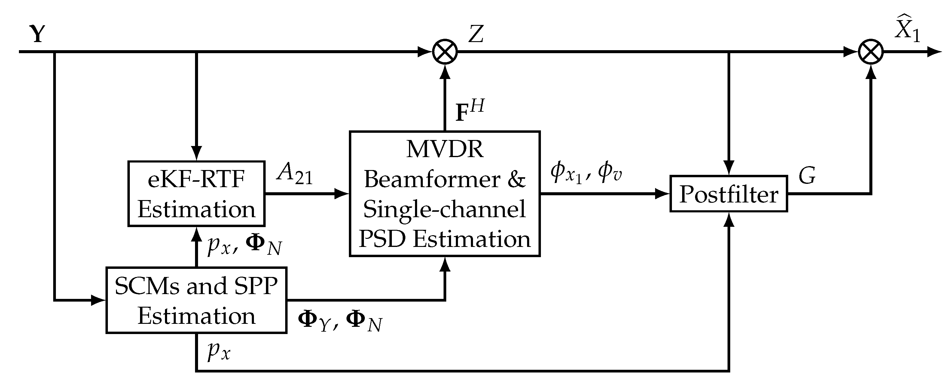
The proposed enhancement system for dual-microphone smartphones is depicted in Figure 1. The microphones capture the noisy speech signals $y_m\left(n\right)$, where m indicates the microphone index ($m=1,2$). We assume an additive noise distortion model which in the short-time Fourier transform (STFT) domain can be expressed as

$$Y_m(t,f)=X_m(t,f)+N_m(t,f),$$

(1)

where $Y_m(t,f)$, $X_m(t,f)$ and $N_m(t,f)$ represent, respectively, noisy speech, clean speech and noise signal STFTs, t is the frame index and f the frequency bin. The two channel components can be stacked in a vector,

$$\mathbf{Y}(t,f)={\left[\begin{array}{ccc}{Y}_1(t,f)& ,& Y_2(t,f)\end{array}\right]}^{\top },$$

(2)

where ${[·]}^{\top }$ indicates matrix transposition. Similarly, we define vectors $\mathbf{X}(t,f)$ and $\mathbf{N}(t,f)$. In the following, we will consider that each frequency component can be processed independently from the others, which is commonly referred to as narrowband approximation [6].

As shown in Figure 1, the beamforming block requires two previous procedures. First, a speech presence probability (SPP)-based algorithm is employed for the estimation of the noisy speech and noise spatial correlation matrices (SCM), ${\mathsf{\Phi }}_Y(t,f)$ and ${\mathsf{\Phi }}_N(t,f)$, respectively, and the SPP, $p_x(t,f)$. Then, an extended Kalman filter (eKF)-based estimator obtains the relative transfer function (RTF) between the secondary microphone ($m=2$) and the reference microphone ($m=1$), defined as

$$A_{21}(f,t)=\frac{X_2(f,t)}{X_1(f,t)}.$$

(3)

Once the SCM matrices and RTF have been computed, the dual-channel noisy speech vector $\mathbf{Y}(t,f)$ is processed using a Minimum Variance Distortionless Response (MVDR) beamformer, which applies spatial filtering yielding an output signal $Z(t,f)$ defined as

$$Z(t,f)={\mathbf{F}}^H(t,f)\mathbf{Y}(t,f),$$

(4)

where ${(·)}^H$ indicates a Hermitian transpose. The coefficients of the beamformer, $\mathbf{F}(t,f)$, are estimated as [2],

$$\mathbf{F}(t,f)=\frac{{\mathsf{\Phi }}_N^{-1}(t,f)\mathbf{d}(t,f)}{{\mathbf{d}}^H(t,f){\mathsf{\Phi }}_N^{-1}(t,f)\mathbf{d}(t,f)},$$

(5)

where

$$\mathbf{d}(t,f)={\left[\begin{array}{ccc}1& ,& A_{21}(t,f)\end{array}\right]}^{\top }$$

(6)

is the steering vector normalized to the reference channel.

Finally, the speech signal at the beamformer output is enhanced by a single-channel postfilter for additional noise reduction. A spectral gain $G(t,f)$ is obtained using the power spectral density (PSD) of the speech at the reference microphone ${\varphi }_{x_1}(t,f)$, the PSD of the residual noise ${\varphi }_v(t,f)$ and the SPP $p_x(t,f)$. The above single-channel statistics (${\varphi }_{x_1}(t,f)$ and ${\varphi }_v(t,f)$) are estimated from the noisy speech and noise SCMs and the RTF. The gain function is further processed by a musical noise reduction algorithm [28] and finally applied to the beamformer output, thus obtaining

$${\widehat{X}}_1(t,f)=G(t,f)Z(t,f),$$

(7)

where ${\widehat{X}}_1(t,f)$ is the estimate of the clean speech signal at the reference microphone. In the following sections, the description of the different parts of the system is addressed.

3. Extended Kalman Filter-Based Relative Transfer Function Estimation

The proposed system requires knowledge of the RTF between the two microphones, namely $A_{21}(f,t)$. Among other approaches, the computation of this RTF can be addressed as the estimation of a variable that changes across frames in terms of a stochastic model. Given this dynamic model, the noise statistics and the noisy observations, we proposed in [15] the tracking of the RTF using an extended Kalman filter (eKF), showing a better estimation performance in comparison with other state-of-the-art approaches. Next, we describe in detail the derivation of this eKF-based RTF estimation.

First, we formulate the narrowband approximation for a given frequency of the noisy speech signal at the secondary microphone in terms of the reference microphone as

$$Y_2\left(t\right)=A_{21}\left(t\right)\left(Y_1\left(t\right)-N_1\left(t\right)\right)+N_2\left(t\right),$$

(8)

where the frequency index f has been omitted for the sake of simplicity. In addition, complex variables are expressed as stacked vectors of their real and imaginary parts. For example, given $Y_m\left(t\right)=Y_{m,t}^r+j{Y}_{m,t}^i$ with $m=1,2$, we can define

$${\mathbf{y}}_{m,t}={\left[\begin{array}{ccc}{Y}_{m,t}^r& ,& Y_{m,t}^i\end{array}\right]}^{\top },$$

(9)

and, in a similar way,

$${\mathbf{a}}_{21,t}={\left[\begin{array}{ccc}{A}_{21,t}^r& ,& A_{21,t}^i\end{array}\right]}^{\top },$$

(10)

$${\mathbf{n}}_{m,t}={\left[\begin{array}{ccc}{N}_{m,t}^r& ,& N_{m,t}^i\end{array}\right]}^{\top }.$$

(11)

Using these definitions for the model variables in terms of vectors, we propose the following dynamic and observation models needed by the Kalman filter:

• Dynamic model for the RTF ${\mathbf{a}}_{21,t}$: We assume that the state vector ${\mathbf{a}}_{21,t}$ is a random walk stochastic process which can be expressed as

  $${\mathbf{a}}_{21,t}={\mathbf{a}}_{21,t-1}+{\mathbf{w}}_t,$$

  (12)

  where

  $${\mathbf{w}}_t\sim \mathcal{N}\left(\mathbf{0},\mathbf{Q}\right)$$

  (13)

  is a zero-mean multivariate white Gaussian noise that models the variability of the RTF. A detailed discussion on this model is provided in Section 3.2.
• Observation model for the noisy speech at the secondary microphone, ${\mathbf{y}}_{2,t}$: It is defined using the distortion model in (8) as

  $$\begin{array}{cc}{\mathbf{y}}_{2,t}\hfill & =\mathbf{h}\left({\mathbf{a}}_{21,t},{\mathbf{n}}_{1,t};{\mathbf{y}}_{1,t}\right)+{\mathbf{n}}_{2,t}\hfill \\ \hfill & =\left(\left[\begin{array}{cc}1& 0\\ 0& 1\end{array}\right]\left(Y_{1,t}^r-N_{1,t}^r\right)+\left[\begin{array}{cc}0& -1\\ 1& 0\end{array}\right]\left(Y_{1,t}^i-N_{1,t}^i\right)\right){\mathbf{a}}_{21,t}+{\mathbf{n}}_{2,t},\hfill \end{array}$$

  (14)

  where the noises are assumed to be zero-mean multivariate Gaussian variables,

  $$\left[\begin{array}{c}{\mathbf{n}}_{1,t}\\ {\mathbf{n}}_{2,t}\end{array}\right]\sim \mathcal{N}\left(\mathbf{0},\left[\begin{array}{cc}{\mathsf{\Sigma }}_{n_{11},t}& {\mathsf{\Sigma }}_{n_{12},t}\\ {\mathsf{\Sigma }}_{n_{21},t}& {\mathsf{\Sigma }}_{n_{22},t}\end{array}\right]\right),$$

  (15)

  where ${\mathsf{\Sigma }}_{n_{ij},t}=E\left[{\mathbf{n}}_{i,t}{\mathbf{n}}_{j,t}^{\top }\right]$ is a noise covariance matrix whose estimation is addressed in Section 4. Additionally, we assume that there is no correlation between ${\mathbf{a}}_{21,t}$ and ${\mathbf{n}}_{m,t}$ while ${\mathbf{n}}_{1,t}$ and ${\mathbf{n}}_{2,t}$ are correlated. The model $\mathbf{h}$ is non linear because of the product between the variables ${\mathbf{a}}_{21,t}$ and ${\mathbf{n}}_{1,t}$. This model depends on the observation ${\mathbf{y}}_{1,t}$, which acts as a model parameter.

Finally, the Kalman filter framework is applied to obtain a (recursive) minimum mean square error (MMSE) estimate of ${\mathbf{a}}_{21,t}$. This is a two-step procedure that is applied frame-by-frame for all frequencies:

• The prediction step, using the model (12), is applied for every frame $t>0$,

  $${\widehat{\mathbf{a}}}_{21,t|t-1}={\widehat{\mathbf{a}}}_{21,t-1},$$

  (16)

  $${\mathbf{P}}_{t|t-1}={\mathbf{P}}_{t-1}+\mathbf{Q},$$

  (17)

  where

  $${\mathbf{P}}_t=E\left[\left({\mathbf{a}}_{21,t}-{\widehat{\mathbf{a}}}_{21,t}\right){\left({\mathbf{a}}_{21,t}-{\widehat{\mathbf{a}}}_{21,t}\right)}^{\top }\right],$$

  (18)

  $${\mathbf{P}}_{t|t-1}=E\left[\left({\mathbf{a}}_{21,t}-{\widehat{\mathbf{a}}}_{21,t|t-1}\right){\left({\mathbf{a}}_{21,t}-{\widehat{\mathbf{a}}}_{21,t|t-1}\right)}^{\top }\right]$$

  (19)

  are error covariance matrices. The Kalman filter is initialized using the overall mean and covariance of the RTF, that is, ${\widehat{\mathbf{a}}}_{21,0}={\mathit{\mu }}_{a_{21}}$ and ${\mathbf{P}}_0={\mathsf{\Sigma }}_{a_{21}}$. Further details about these parameters are provided in Section 3.2.
• The updating step is applied to correct the previous estimation with the observations ${\mathbf{y}}_{1,t}$ and ${\mathbf{y}}_{2,t}$ (whose relationship is given by Equation (14)),

  $${\widehat{\mathbf{a}}}_{21,t}={\widehat{\mathbf{a}}}_{21,t|t-1}+{\mathbf{K}}_t\left({\mathbf{y}}_{2,t}-{\mathit{\mu }}_{y,t}\right),$$

  (20)

  $${\mathbf{P}}_t={\mathbf{P}}_{t|t-1}-{\mathbf{K}}_t{\mathbf{S}}_{y,t}{\mathbf{K}}_t^{\top },$$

  (21)

  where

  $${\mathbf{K}}_t={\mathbf{C}}_{ay,t}{\mathbf{S}}_{y,t}^{-1}$$

  (22)

  is the Kalman gain, and

  $${\mathit{\mu }}_{y,t}=E\left[{\mathbf{y}}_{2,t}\right],$$

  (23)

  $${\mathbf{S}}_{y,t}=E\left[\left({\mathbf{y}}_{2,t}-{\mathit{\mu }}_{y,t}\right){\left({\mathbf{y}}_{2,t}-{\mathit{\mu }}_{y,t}\right)}^{\top }\right],$$

  (24)

  $${\mathbf{C}}_{ay,t}=E\left[\left({\mathbf{a}}_{21,t}-{\widehat{\mathbf{a}}}_{21,t|t-1}\right){\left({\mathbf{y}}_{2,t}-{\mathit{\mu }}_{y,t}\right)}^{\top }\right]$$

  (25)

  are necessary statistics, the estimation of which is developed in the next subsection. These equations correspond to the most general Kalman filter model as described in Reference [29]. We define the equations in terms of ${\mathit{\mu }}_{y,t}$, ${\mathbf{S}}_{y,t}$ and ${\mathbf{C}}_{ay,t}$ because the non-linearity of $\mathbf{h}$ in Equation (14) makes their estimation non-trivial.

To deal with non-linear functions, two variants of the Kalman filter are widely used: the eKF and the unscented Kalman filter (uKF) [29]. In the case of the model of (14), it could be demonstrated that both eKF and uKF yield the same closed-form expressions for ${\mathit{\mu }}_{y,t}$, ${\mathbf{S}}_{y,t}$ and ${\mathbf{C}}_{ay,t}$. We choose the eKF approach because it gives a more stable computational solution and it is easier to implement than the uKF one. In the next subsection the eKF approach is presented.

3.1. Vector Taylor Series Approximation

The eKF is based on applying a linearization over the prediction and observation models using first-order vector Taylor series (VTS). In our case, the prediction model is linear, so the linearization is only applied to function $\mathbf{h}$ in the observation model. The first-order VTS approximates the model of Equation (14) as

$${\mathbf{y}}_{2,t}\simeq \mathbf{h}\left({\widehat{\mathbf{a}}}_{21,t|t-1},\mathbf{0};{\mathbf{y}}_{1,t}\right)+{\mathbf{H}}_t\left({\mathbf{a}}_{21,t}-{\widehat{\mathbf{a}}}_{21,t|t-1}\right)+{\mathbf{J}}_{n_1,t}{\mathbf{n}}_{1,t}+{\mathbf{n}}_{2,t},$$

(26)

where

$${\mathbf{H}}_t={\left.\frac{\partial \mathbf{h}}{\partial {\mathbf{a}}_{21,t}}\right|}_{{\mathbf{n}}_{1,t}=\mathbf{0}}=\left[\begin{array}{cc}{Y}_{1,t}^r& -Y_{1,t}^i\\ Y_{1,t}^i& Y_{1,t}^r\end{array}\right],$$

(27)

$${\mathbf{J}}_{n_1,t}={\left.\frac{\partial \mathbf{h}}{\partial {\mathbf{n}}_{1,t}}\right|}_{{\mathbf{a}}_{21,t}={\widehat{\mathbf{a}}}_{21,t|t-1}}=-\left[\begin{array}{cc}{\widehat{A}}_{21,t|t-1}^r& -{\widehat{A}}_{21,t|t-1}^i\\ {\widehat{A}}_{21,t|t-1}^i& {\widehat{A}}_{21,t|t-1}^r\end{array}\right]$$

(28)

are the Jacobian matrices required for the VTS approach.

Finally, using (26), the noisy speech statistics can be estimated as [29]

$${\mathit{\mu }}_{y,t}\simeq \mathbf{h}\left({\widehat{\mathbf{a}}}_{21,t|t-1},\mathbf{0};{\mathbf{y}}_{1,t}\right),$$

(29)

$${\mathbf{S}}_{y,t}\simeq {\mathbf{H}}_t{\mathbf{P}}_{t|t-1}{\mathbf{H}}_t^{\top }+{\mathbf{J}}_{n_1,t}{\mathsf{\Sigma }}_{n_{11},t}{\mathbf{J}}_{n_1,t}^{\top }+{\mathsf{\Sigma }}_{n_{22},t}+{\mathbf{J}}_{n_1,t}{\mathsf{\Sigma }}_{n_{12},t}+{\mathsf{\Sigma }}_{n_{21},t}{\mathbf{J}}_{n_1,t}^{\top },$$

(30)

$${\mathbf{C}}_{ay,t}\simeq {\mathbf{P}}_{t|t-1}{\mathbf{H}}_t^{\top }.$$

(31)

3.2. A Priori RTF Statistics

The dynamic model for the RTF vector ${\mathbf{a}}_{21,t}$ presented in Equation (12) accounts for the process variability across time in terms of a white noise ${\mathbf{w}}_t$. This variability has a twofold meaning: first, the possible temporal variations of the acoustic channel due to environment changes, head or smartphone movements, etc., and, second, the inaccuracy of the narrowband approximation of Equation (8) [6]. This is due to the fact that, especially in reverberant environments where the analysis window of the STFT is shorter than the impulse response of the acoustic channel, the transfer function is not multiplicative but convolutive. This convolutive transfer function expands in both time and frequency dimensions. Thus, nearby frames and frequencies are correlated, which violates the narrowband approximation [6]. In order to account for the variability associated to this effect, we will assume the statistical model proposed in (12) so that, although the channel could be time-invariant, the RTF, as defined in Equation (3), is time-variant.

The eKF-based RTF estimator requires the a priori statistics of the RTF. These statistics are the overall mean vector and covariance matrix of the RTF, respectively,

$${\mathit{\mu }}_{a_{21}}=E\left[{\mathbf{a}}_{21,t}\right],$$

(32)

$${\mathsf{\Sigma }}_{a_{21}}=E\left[\left({\mathbf{a}}_{21,t}-{\mathit{\mu }}_{a_{21}}\right){\left({\mathbf{a}}_{21,t}-{\mathit{\mu }}_{a_{21}}\right)}^{\top }\right],$$

(33)

and also the covariance of the RTF variability across frames,

$$\mathbf{Q}=E\left[{\mathbf{w}}_t{\mathbf{w}}_t^{\top }\right]=E\left[\left({\mathbf{a}}_{21,t}-{\mathbf{a}}_{21,t-1}\right){\left({\mathbf{a}}_{21,t}-{\mathbf{a}}_{21,t-1}\right)}^{\top }\right].$$

(34)

Additionally, we can define the overall correlation matrix of the RTF as

$${\mathbf{R}}_{a_{21}}=E\left[{\mathbf{a}}_{21,t}{\mathbf{a}}_{21,t}^{\top }\right]={\mathsf{\Sigma }}_{a_{21}}+{\mathit{\mu }}_{a_{21}}{\mathit{\mu }}_{a_{21}}^{\top }.$$

(35)

The previous statistics can be estimated in advance using a training set of dual-channel clean speech utterances in different acoustic environments and device positions. In order to avoid outliers which might yield useless estimates, we select, on an utterance basis, time-frequency bins where the speech power at the reference channel is large enough (higher than the maximum power at that frequency in the utterance minus 3 dB). For those bins, we estimate the RTF using (3), which yields a set of RTFs $A_{21}^{\left(l\right)}(t,f)$ for the l-th utterance, that are later converted to RTF vectors ${\mathbf{a}}_{21,t}^{\left(l\right)}$. For each utterance, a sample mean vector ${\widehat{\mathit{\mu }}}_{a_{21}}^{\left(l\right)}$ and a sample correlation matrix ${\widehat{\mathbf{R}}}_{a_{21}}^{\left(l\right)}$ are estimated using those ${\mathbf{a}}_{21,t}^{\left(l\right)}$ vectors, while a sample covariance matrix ${\widehat{\mathbf{Q}}}^{\left(l\right)}$ is computed from consecutive RTF vectors. Finally, the global sample statistics ${\widehat{\mathit{\mu }}}_{a_{21}}$, ${\widehat{\mathbf{R}}}_{a_{21}}$ and $\widehat{\mathbf{Q}}$ are obtained by averaging the particular utterance-dependent statistics. The sample covariance ${\widehat{\mathsf{\Sigma }}}_{a_{21}}$ can then be estimated using ${\widehat{\mathit{\mu }}}_{a_{21}}$ and ${\widehat{\mathbf{R}}}_{a_{21}}$ in (35).

4. Speech Presence Probability-Based Noise Statistics Estimation

The eKF-RTF estimator and the beamforming algorithm also require knowledge of the noise spatial correlation matrix (SCM) ${\mathsf{\Phi }}_N(t,f)$. In this work, we follow the multi-channel speech presence probability (SPP) approach described in Reference [4]. This estimation method is based on the recursive updating of the noise SCM in those time-frequency bins where speech is absent. First, two hypotheses, $H_x$ and $H_n$, are considered for speech presence and speech absence, respectively,

$$H_x:\mathbf{Y}(t,f)=\mathbf{X}(t,f)+\mathbf{N}(t,f),$$

(36)

$$H_n:\mathbf{Y}(t,f)=\mathbf{N}(t,f).$$

(37)

Assuming zero-mean random variables, the SCM of the noise will be updated by means of the following recursion,

$${\widehat{\mathsf{\Phi }}}_N(t,f)=\alpha (t,f){\widehat{\mathsf{\Phi }}}_N(t-1,f)+\left(1-\alpha (t,f)\right)\mathbf{Y}(t,f){\mathbf{Y}}^H(t,f),$$

(38)

where the forgetting factor is computed as

$$\alpha (t,f)=\tilde{\alpha }+p_x(t,f)\left(1-\tilde{\alpha }\right),$$

(39)

where $\tilde{\alpha }\in \left[0,1\right)$ is an updating constant and

$$p_x(t,f)=P\left(H_x|\mathbf{Y}(t,f)\right)$$

(40)

is the a posteriori SPP. The estimation of this probability is detailed in Section 4.1.

From now on, the time and frequency indices are omitted whenever possible. The noise statistics for the RTF estimator (required by (30)) are directly derived from ${\mathsf{\Phi }}_N$. Assuming a zero-mean, symmetric circular complex Gaussian distribution for $\mathbf{N}$ [30] and

$${\mathsf{\Phi }}_N=\left[\begin{array}{cc}{\varphi }_{N_{11}}& {\varphi }_{N_{12}}\\ {\varphi }_{N_{21}}& {\varphi }_{N_{22}}\end{array}\right],$$

(41)

with ${\varphi }_{N_{ij}}=E\left[N_i{N}_j^{*}\right]$, the following relations can be demonstrated,

$${\mathsf{\Sigma }}_{n_{11}}=\frac{1}{2}{\varphi }_{N_{11}}{\mathbf{I}}_2,$$

(42)

$${\mathsf{\Sigma }}_{n_{22}}=\frac{1}{2}{\varphi }_{N_{22}}{\mathbf{I}}_2,$$

(43)

$${\mathsf{\Sigma }}_{n_{12}}=\frac{1}{2}\left[\begin{array}{cc}{\varphi }_{N_{12}}^r& -{\varphi }_{N_{12}}^i\\ {\varphi }_{N_{12}}^i& {\varphi }_{N_{12}}^r\end{array}\right],$$

(44)

$${\mathsf{\Sigma }}_{n_{21}}={\mathsf{\Sigma }}_{n_{12}}^{\top },$$

(45)

where ${\mathbf{I}}_2$ is the 2-dimensional identity matrix.

4.1. A Posteriori SPP Estimation

The a posteriori SPP $p_x(t,f)$ allows us to control the updating procedure of Equation (38) for the computation of the noise statistics. Nevertheless, $p_x(t,f)$ is also exploited in two additional parts of our system:

• The estimation of the RTF presented in the previous section is only accurate in time-frequency bins where speech is present. The a posteriori SPP indicates those bins where speech presence is more likely. Therefore, in our implementation we only update the eKF in those bins where $p_x(t,f)>p_{\mathrm{thr}}$, with $p_{\mathrm{thr}}$ being a predefined probability threshold. Otherwise, the previous values are preserved.
• The postfiltering performance can be improved if additional information about SPP is provided, as shown later in Section 5.

The estimation of the a posteriori SPP can be addressed assuming complex multivariate Gaussian distributions for the noisy speech $\mathbf{Y}$ [4,5], according to the two hypotheses previously formulated (see (36) and (37)). Using the Bayes’ rule, the a posteriori SPP at each time-frequency bin can be calculated as

$$p_x=\frac{\left(1-q_n\right)f\left(\mathbf{Y}|H_x\right)}{\left(1-q_n\right)f\left(\mathbf{Y}|H_x\right)+q_{n}f\left(\mathbf{Y}|H_n\right)},$$

(46)

where $q_n=P\left(H_n\right)$ is the a priori speech absence probability (SAP) and

$$f\left(\mathbf{Y}|H_x\right)=\frac{e^{-\mathbf{Y}{\mathsf{\Phi }}_Y^{-1}{\mathbf{Y}}^H}}{{\pi }^{M}det\left[{\mathsf{\Phi }}_Y\right]},$$

(47)

$$f\left(\mathbf{Y}|H_n\right)=\frac{e^{-\mathbf{Y}{\mathsf{\Phi }}_N^{-1}{\mathbf{Y}}^H}}{{\pi }^{M}det\left[{\mathsf{\Phi }}_N\right]},$$

(48)

are the likelihoods of observing the noisy speech signal under the different hypotheses, with $det\left[·\right]$ being the matrix determinant operator and M the number of microphones. Equation (46) can be redefined using these likelihoods, yielding the following expression for the SPP,

$$p_x={\left(1+\frac{q_n}{1-q_n}\frac{det\left[{\mathsf{\Phi }}_Y\right]}{det\left[{\mathsf{\Phi }}_N\right]}\frac{e^{-\mathbf{Y}{\mathsf{\Phi }}_N^{-1}{\mathbf{Y}}^H}}{e^{-\mathbf{Y}{\mathsf{\Phi }}_Y^{-1}{\mathbf{Y}}^H}}\right)}^{-1}.$$

(49)

Then, the a posteriori SPP can be estimated at each frame for all frequencies according to the following two-iteration algorithm:

• Initialization: Estimate the noisy SCM with a recursive updating,

  $${\widehat{\mathsf{\Phi }}}_Y(t,f)=\tilde{\alpha }{\widehat{\mathsf{\Phi }}}_Y(t-1,f)+\left(1-\tilde{\alpha }\right)\mathbf{Y}(t,f){\mathbf{Y}}^H(t,f),$$

  (50)

  where $\tilde{\alpha }$ is an updating constant as in (39). Also, estimate the a priori SAP $q_n(t,f)$ (see Section 4.2).
• 1st iteration: Estimate $p_x(t,f)$ using ${\widehat{\mathsf{\Phi }}}_N(t-1,f)$ in (49). Then, estimate ${\widehat{\mathsf{\Phi }}}_N(t,f)$ using $p_x(t,f)$ in (38).
• 2nd iteration: Re-estimate $p_x(t,f)$ using now ${\widehat{\mathsf{\Phi }}}_N(t,f)$ in (49). Finally, re-estimate ${\widehat{\mathsf{\Phi }}}_N(t,f)$ using $p_x(t,f)$.

4.2. A Priori SAP Estimation

To obtain an accurate a posteriori SPP that allows for robust tracking of the noise statistics, the a priori SAP is a key parameter. Methods on single-channel noise tracking, as the fixed a priori SNR algorithm of Reference [31] or the minima controlled recursive averaging (MCRA) algorithm [32], estimate this SAP in terms of the a priori SNR. The MCRA framework was extended to multi-channel speech signals in Reference [4]. This is the SPP estimator that we used in our previous works [15,27]. A major drawback of the MCRA scheme is the lack of robustness in case of a time-varying SNR, which makes noise changes to be detected as speech presence. More recently, the authors of [5] proposed to use spatial information in the SAP estimation, specifically the coherent-to-diffuse ratio (CDR). Alternatively, the power level difference (PLD) between microphones is used in Reference [17] to update the noise statistics, as it is a good indicator of speech presence in CT conditions. In this work, we propose a novel SAP estimator for dual-microphone smartphones that combines the CDR spatial information with the PLD between the reference and the secondary microphones.

First, an SCM ${\tilde{\mathsf{\Phi }}}_Y(t,f)$ is estimated using a rectangular window of eight past frames as in Reference [5]. Then, we calculate (1) the power spectral density (PSD) ratio between microphones as

$${\widehat{\sigma }}_{Y_{21}}(t,f)=\frac{{\tilde{\varphi }}_{Y_{22}}(t,f)}{{\tilde{\varphi }}_{Y_{11}}(t,f)},$$

(51)

where ${\tilde{\varphi }}_{Y_{ij}}$ is an estimate of $E\left[Y_i{Y}_j^{*}\right]$, and (2) the short-term complex coherence between microphones,

$${\widehat{\psi }}_{Y_{12}}(t,f)=\frac{{\tilde{\varphi }}_{Y_{12}}(t,f)}{\sqrt{{\tilde{\varphi }}_{Y_{11}}(t,f){\tilde{\varphi }}_{Y_{22}}(t,f)}}.$$

(52)

Both terms are needed by the SAP estimators.

The PLD-based a priori SAP is based on the PLD noise estimator for CT conditions described in Reference [17]. In that work, a normalized difference of the noisy speech PSDs was defined as

$$\Delta {\widehat{\varphi }}_{\mathrm{nPLD}}(t,f)=\frac{{\tilde{\varphi }}_{Y_{11}}(t,f)-{\tilde{\varphi }}_{Y_{22}}(t,f)}{{\tilde{\varphi }}_{Y_{11}}(t,f)+{\tilde{\varphi }}_{Y_{22}}(t,f)}=\frac{1-{\widehat{\sigma }}_{Y_{21}}(t,f)}{1+{\widehat{\sigma }}_{Y_{21}}(t,f)}.$$

(53)

The noise statistics are updated by this parameter, as it gives information about speech presence. That is, assuming similar noise power at both microphones and that speech is more attenuated at the secondary microphone with respect to the primary one, $\Delta {\widehat{\varphi }}_{\mathrm{nPLD}}(t,f)$ is close to one when speech is present and tends to zero otherwise. Thus, an a priori SAP based on this indicator can be estimated as

$$q_{\mathrm{PLD}}(t,f)=1-\Delta {\widehat{\varphi }}_{\mathrm{nPLD}}(t,f)=\frac{2{\widehat{\sigma }}_{Y_{21}}(t,f)}{1+{\widehat{\sigma }}_{Y_{21}}(t,f)},$$

(54)

where $q_{\mathrm{PLD}}(t,f)$ is upper-bounded by 1. This estimator is valid for CT conditions, but it can also be useful in FT conditions for frequencies where speech at the secondary microphone is attenuated.

On the other hand, the CDR is another good indicator of speech presence [33], which is defined as

$${\mathrm{\Gamma }}_{Y_{12}}(t,f)=\frac{{\psi }_{\mathrm{diff}}\left(f\right)-{\psi }_{Y_{12}}(t,f)}{{\psi }_{Y_{12}}(t,f)-{\psi }_{X_{12}}(t,f)},$$

(55)

where ${\psi }_{X_{12}}(t,f)$ is the clean speech short-term complex coherence (defined as in (52)) and

$${\psi }_{\mathrm{diff}}\left(f\right)=\mathrm{sinc}\left(\frac{2\pi f{F}_s{d}_{\mathrm{mic}}}{K{c}_v}\right)$$

(56)

is the diffuse noise field complex coherence, with $F_s$ the sampling frequency, K the number of frequency bins, $d_{\mathrm{mic}}$ the distance between microphones and $c_v$ the speed of sound. While higher values of the CDR indicate the presence of a strong coherent component, often a speech signal, lower values indicate that a diffuse component is dominant, which is more common for noise signals. In practice, the CDR is obtained using the estimator proposed in Reference [33],

$${\widehat{\mathrm{\Gamma }}}_{Y_{12}}(t,f)=\Re \left(\frac{{\psi }_{\mathrm{diff}}\left(f\right)-{\widehat{\psi }}_{Y_{12}}(t,f)}{{\widehat{\psi }}_{Y_{12}}(t,f)-e^{j\angle {\tilde{\varphi }}_{Y_{12}}(t,f)}}\right),$$

(57)

where $\angle {\tilde{\varphi }}_{Y_{12}}(t,f)$ is the phase of ${\tilde{\varphi }}_{Y_{12}}(t,f)$. Although the CDR is positive and real-valued, estimation errors yield complex-valued results, so the real-part $\Re \left(·\right)$ is taken in (57). Additionally, a frequency-averaged CDR with a normalized Hamming window $h_W$ is computed as

$${\overline{\mathrm{\Gamma }}}_{Y_{12}}(t,f)=\sum _{i=-w}^w{h}_W\left(i\right){\widehat{\mathrm{\Gamma }}}_{Y_{12}}(t,f-i),$$

(58)

with $w=10$ (the window width is $2w+1$). Then, the local a priori SAP estimate is obtained as in Reference [5] using ${\widehat{\mathrm{\Gamma }}}_{Y_{12}}(t,f)$,

$$q_{\mathrm{local}}(t,f)=q_{min}+\left(q_{max}-q_{min}\right)\frac{{10}^{\frac{c\rho }{10}}}{{10}^{\frac{c\rho }{10}}+{\widehat{\mathrm{\Gamma }}}_{Y_{12}}^{\rho }(t,f)},$$

(59)

where $q_{min}$ and $q_{max}$ define the minimum and maximum values of the function, respectively, c is an offset parameter and $\rho$ controls the steepness of the transition region. Similarly, the global a priori SAP estimate $q_{\mathrm{global}}(t,f)$ is computed using ${\overline{\mathrm{\Gamma }}}_{Y_{12}}(t,f)$ in (59). The CDR-based a priori SAP is then obtained as in Reference [5],

$$q_{\mathrm{CDR}}(t,f)=1-(1-q_{\mathrm{local}}(t,f))(1-q_{\mathrm{global}}(t,f)).$$

(60)

This estimator is the same as that proposed in Reference [5], except for the term representing the frame a priori SAP. This term was neglected as it did not increase the performance in our preliminary experiments.

Finally, the a priori SAP estimates obtained by PLD and CDR are combined to achieve a more robust joint decision. Assuming statistical independence between both estimators, the final a priori SAP estimate for dual-microphone smartphones is calculated as the joint probability of the speech absence decision by each estimator,

$$q_n(t,f)=q_{\mathrm{CDR}}(t,f)q_{\mathrm{PLD}}(t,f).$$

(61)

The above estimator can be used in both CT and FT conditions to obtain prior information about speech presence. Moreover, as it only allows for noise statistics updating when both estimates indicate speech absence, this estimator is expected to be more robust.

5. Postfiltering Approaches for Dual-Microphone Smartphones

As introduced above, the performance achieved by beamforming algorithms is limited in our scenario mainly due to the reduced number of microphones and the particular placement on the smartphone. In this section we propose different alternatives for single-channel postfiltering at the beamformer output. These postfilters make use of the previously estimated parameters to design a gain function which is applied to the beamformer output signal for further noise reduction. In the next subsections we describe several postfiltering techniques as well as our proposals for the estimation of the clean speech and noise single-channel statistics required by the former ones.

5.1. Parametric Wiener Filtering

Under the distortionless constraint of MVDR, if we assume an accurate estimation of the RTF, we can approximate the single-channel speech signal $Z(t,f)$ at the beamformer output as

$$Z(t,f)\simeq X_1(t,f)+V(t,f),$$

(62)

where $V(t,f)$ is the residual noise at the beamformer output,

$$V(t,f)={\mathbf{F}}^H(t,f)\mathbf{N}(t,f).$$

(63)

The PSDs of the clean speech signal $X_1(t,f)$ and the residual noise $V(t,f)$ are given by ${\varphi }_{x_1}(t,f)$ and ${\varphi }_v(t,f)$, respectively. The corresponding Wiener filter (WF) for $X_1(t,f)$ is then defined as

$$G(t,f)=\frac{\xi (t,f)}{1+\xi (t,f)},$$

(64)

where

$$\xi (t,f)=\frac{{\varphi }_{x_1}(t,f)}{{\varphi }_v(t,f)}$$

(65)

is the a priori SNR.

The noise reduction performance of WF can be improved if we consider the a posteriori SPP $p_x(t,f)$ in the postfiltering design. Our goal is to decrease the gain factor for time-frequency bins where speech is absent. This yields the parametric WF (pWF) [34]

$$G(t,f)=\frac{\xi (t,f)}{\mu (t,f)+\xi (t,f)},$$

(66)

where $\mu (t,f)$ is an SPP-driven trade-off parameter. To obtain this parameter, we use the same mapping function as in Reference [5],

$$\mu (t,f)={\mu }_{min}+\left({\mu }_{max}-{\mu }_{min}\right)\frac{{10}^{\frac{c\rho }{10}}}{{10}^{\frac{c\rho }{10}}+{\left(\frac{p_x(t,f)}{1-p_x(t,f)}\right)}^{\rho }},$$

(67)

which is similar to the mapping function of (59). We can see that $\mu (t,f)\in \left[{\mu }_{min},{\mu }_{max}\right]$ and therefore, the lower the a posteriori SPP, the higher $\mu (t,f)$, thus improving the noise reduction performance.

5.2. Optimally Modified Log-Spectral Amplitude Estimator

Instead of estimating a WF filter over the signal statistics, other approaches try to directly make an MMSE estimation of the clean speech signal amplitude $\left|X_1(t,f)\right|$. One of these is the log-spectral amplitude (LSA) estimator proposed in Reference [35] and defined as

$$\left|{\widehat{X}}_1(t,f)\right|=exp\left(E\left[\left.log\left(\left|X_1(t,f)\right|\right)\right|Z(t,f)\right]\right)=G_{H_x}(t,f)\left|Z(t,f)\right|,$$

(68)

where

$$G_{H_x}(t,f)=\frac{\xi (t,f)}{1+\xi (t,f)}exp\left(\frac{1}{2}{\int }_{\frac{\xi (t,f)}{1+\xi (t,f)}\gamma (t,f)}^{\infty }\frac{e^{-u}}{u}du\right)$$

(69)

is the LSA gain function, and

$$\gamma (t,f)=\frac{{\left|Z(t,f)\right|}^2}{{\varphi }_v(t,f)}$$

(70)

is the a posteriori SNR. As can be seen, this estimator is equivalent to applying a gain function over the noisy speech signal $Z(t,f)$ that depends not only on the a priori SNR but also on the a posteriori SNR. The obtained gain function is similar to WF for high a priori SNRs and has lower values than WF when the a priori SNR is lower and the a posteriori SNR is higher (i.e., when noise tends to dominate).

The estimator of (68) is only valid under the assumption of speech presence. To improve the performance, the authors of Reference [36] proposed a different estimator that also takes into account the a posteriori SPP and different gain functions for speech presence and absence. That is the optimally modified LSA (OMLSA) estimator, which is defined as

$$G(t,f)=G_{H_x}{(t,f)}^{p_x(t,f)}{G}_{H_v}{(t,f)}^{1-p_x(t,f)},$$

(71)

where $G_{H_v}$ is a constant attenuation applied when speech is absent, whose value is usually $-25$ dB [36].

5.3. Single-Channel Speech and Noise PSD Estimators

The computation of the gain functions previously presented relies on the estimation of the single-channel PSDs of the clean speech at the reference channel ${\varphi }_{x_1}(t,f)$ and the residual noise at the beamformer output ${\varphi }_v(t,f)$. The estimation of the residual noise PSD is straightforward if estimates of the SCM ${\mathsf{\Phi }}_N(t,f)$ and the steering vector $\mathbf{d}(t,f)$ are available. In this case, the residual noise PSD can be obtained at each time-frequency bin as

$${\widehat{\varphi }}_v={\left({\widehat{\mathbf{d}}}^H{\widehat{\mathsf{\Phi }}}_N^{-1}\widehat{\mathbf{d}}\right)}^{-1}.$$

(72)

On the other hand, a clean speech PSD estimate is more difficult to obtain because of its higher variability. In Reference [27], we proposed two different estimators that make use of the noisy speech and noise statistics and the RTF between microphones. In the following, we describe both clean speech PSD estimators, omitting time and frequency indices for simplicity.

5.3.1. Power Level Difference-Based Estimation

The PLD-based estimator is derived from the method in Reference [17], which exploits the PLD between the microphones of a smartphone used in CT conditions; that is, a more attenuated clean speech component is expected at the secondary microphone with respect to the primary one. This PLD is defined in terms of the noisy speech PSDs at the microphone inputs,

$$\Delta {\widehat{\varphi }}_{\mathrm{PLD}}=max\left({\widehat{\varphi }}_{Y_{11}}-{\widehat{\varphi }}_{Y_{22}},0\right),$$

(73)

where it is assumed that the power at the reference microphone is always higher than the one at the secondary microphone. Assuming that the noise PSD difference ($\Delta {\varphi }_N={\varphi }_{N_{11}}-{\varphi }_{N_{22}}$) can be neglected when compared to $\Delta {\widehat{\varphi }}_{\mathrm{PLD}}$, the clean speech PSD can be estimated as in [17],

$${\widehat{\varphi }}_{x_1}=\frac{\Delta {\widehat{\varphi }}_{\mathrm{PLD}}}{1-|{\widehat{A}}_{21}{|}^2}.$$

(74)

Although this estimator offers good performance in CT conditions, the previous assumptions are not longer valid in FT conditions.

5.3.2. Minimum Variance Distortionless Response-Based Estimation

This estimator calculates the PSD directly at the beamformer output by spectral subtraction, taking into account the distortionless property of MVDR. The estimator is defined as

$${\widehat{\varphi }}_{x_1}={\mathbf{F}}^H\left({\widehat{\mathsf{\Phi }}}_Y-{\widehat{\mathsf{\Phi }}}_N\right)\mathbf{F},$$

(75)

so that it fully exploits the spatial information by using the SCM matrices of the noisy speech and noise signals. The combination of both channels by means of the beamformer weights ($\mathbf{F}$) allows for a more robust estimation than directly taking the first element of ${\widehat{\mathsf{\Phi }}}_Y-{\widehat{\mathsf{\Phi }}}_N$. Negative PSDs may be obtained due to the estimator variance, so (75) is bounded by 0.

6. Experimental Evaluation

The performance of the different estimators and speech enhancement algorithms discussed along this paper is evaluated by means of objective speech quality and intelligibility metrics. Two different well-known objective metrics are used:

• The Perceptual Evaluation Speech Quality (PESQ) [37] metric is utilized to evaluate the speech quality of the enhanced speech signal. This metric gives a mean opinion score between one and five. The higher the PESQ values, the better the speech quality.
• The Short-Time Objective Intelligibility (STOI) [38] metric is intended to evaluate the speech intelligibility of the enhanced speech signal. The resulting score is a value between zero and one. The higher the STOI value, the better the speech intelligibility.

PESQ and STOI are both intrusive metrics, which means that they need a clean reference. As a reference, we use the clean speech signal at the reference microphone, $x_1\left(n\right)$.

Additionally, in order to evaluate the RTF estimation accuracy, we use the speech distortion (SD) index [2]. This index measures the distortion level on the clean speech signal at the beamformer output, namely ${\tilde{x}}_1\left(n\right)$ (inverse STFT of ${\mathbf{F}}^H(t,f)\mathbf{X}(t,f)$). The idea behind using this metric is that, because of the distortionless property of MVDR, more accurate RTF estimates should yield lower speech distortion. The SD index is measured segmentally across the speech signal, in such a way that the SD value at the i-th segment is obtained as

$$SD\left(i\right)=\frac{{\displaystyle \sum _{n=(i-1)T}^{iT-1}}{\left|x_1\left(n\right)-{\tilde{x}}_1\left(n\right)\right|}^2}{{\displaystyle \sum _{n=(i-1)T}^{iT-1}}{\left|x_1\left(n\right)\right|}^2},$$

(76)

where T is the number of samples per segment. The segmental SD values are averaged to achieve the final SD index, which is a value between zero and one. The lower the SD value, the lower the speech distortion. As in Reference [5], silence frames are excluded from this evaluation by means of calculating the median of the segment-wise signal power and removing those segments with a power 15 dB lower than that median.

We evaluate the proposed algorithms by using simulated dual-channel noisy speech recordings from a dual-microphone smartphone. Two different databases were developed for each device use mode: close-talk (CT) and far-talk (FT). To simulate the recordings, clean speech signals are filtered using dual-channel acoustic impulse responses and real dual-channel environmental noise is added at different signal-to-noise ratios (SNRs). We evaluate four different reverberation environments and eight different noises, which are matched as indicated in

Table 1. Predefined acoustic environments: each environment combines a reverberation environment with a given noise.

Reverberation	Noise (Test Only)
(A) No reverb.	Car, Street, Pedestrian street
(B) Low	Bus, Cafe
(C) Medium	Babble, Bus station
(D) High	Mall

, yielding eight different acoustic environments (including both reverberation and noise). Details about the methodology used to obtain the acoustic impulse responses and the noises can be found in References [15,39].

Clean speech signals are obtained from the TIMIT database [40,41] and downsampled to 16 kHz. In particular, a total of 850 clean speech utterances from different speakers are employed. All the utterances have a length of around seven seconds, which is achieved by same-speaker utterance concatenation. Two different sets are then defined, namely training and test. Speakers do not overlap across sets. Moreover, the number of utterances from female and male speakers is balanced. The distribution of utterances and the number of speakers in the training and test sets are indicated in

Table 2. Distribution of clean speech utterances and speakers across training and test sets.

	N° Utterances	N° Speakers
Training set	700	440
Test set	150	93

.

The training set consists of reverberated clean speech utterances and is only used to estimate the a priori statistics for the eKF-RTF estimator. Such utterances were obtained by filtering each clean speech utterance with a set of dual-channel acoustic impulse responses which model four reverberant environments, thereby yielding a total of 2800 training utterances. Sixteen different acoustic impulse responses were considered for each acoustic environment. For each utterance, the impulse response was randomly selected.

On the other hand, the test set consists of utterances contaminated according to the eight noisy environments defined in Table 1. This set is intended to evaluate the different algorithms proposed in this work. Noises were added to the reverberated speech at six different SNRs from −5 dB to 20 dB, so a total of 7200 test utterances was obtained. In order to simulate reverberation, ten different acoustic impulse responses, in turn also different from those of the training set, were considered for each acoustic environment and, again, randomly applied.

For STFT computation, a 512-point DFT was applied using a 32 ms square-root Hann window with 50% overlap. This results in a total of 257 frequency bins for each time frame. The noisy speech and noise SCMs were estimated using an updating constant $\tilde{\alpha }=0.9$. The parameters for CDR-based a priori SAP calculation were set as [5]: $d_{mic}=13$ cm, $q_{min}=0.1$, $q_{max}=0.998$, $c=3$ and $\rho =2.5$. The SPP threshold for RTF updating was set as $p_{\mathrm{thr}}=0.9$. Finally, for the SPP-driven trade-off parameter of the parametric Wiener filter, the following parameter values were used [5]: ${\mu }_{min}=1$, ${\mu }_{max}=4$, $c=-3$ and $\rho =4$.

The algorithm was implemented in Python and it is available at [42]. The computational burden of the implementation was evaluated on a PC with an Intel Core i7-4790 CPU. The algorithm works on a frame-by-frame basis, so that the algorithmic delay is in this case the duration of a frame, that is, 32 ms. The average performance of the whole system (i.e., including SPP and RTF estimation, MVDR beamforming and postfiltering) on this machine achieved approximately 8x faster than real-time.

In the following, the performance of the different techniques is tested. In order to simplify the reading of the results tables, an acronym is provided (in parentheses) for each considered technique after its description.

6.1. Experimental Results: Performance of SAP Estimators

First, we compare the different a priori SAP estimators when used along with our eKF-RTF estimator for MVDR beamforming (i.e., no postfilter is applied yet). This comparison is shown in

Table 3. Perceptual Evaluation Speech Quality (PESQ) and Short-Time Objective Intelligibility (STOI) results for different speech absence probability (SAP) estimators when combined with speech presence probability (SPP)-based extended Kalman filter - relative transfer function (eKF-RTF) estimation for Minimum Variance Distortionless Response (MDVR) beamforming. Results are broken down by both signal-to-noise ratio (SNR) and device placement.

Place.	Method	PESQ						STOI (%)
		SNR (dB)						SNR (dB)
		20	15	10	5	0	−5	20	15	10	5	0	−5
CT	Noisy	2.26	1.80	1.46	1.23	1.11	1.07	95.36	91.01	83.82	74.05	62.48	51.46
	eKF-MCRA	2.28	1.84	1.49	1.26	1.13	1.08	95.58	91.91	85.37	75.57	63.65	52.20
	eKF-CDR	2.42	2.00	1.63	1.35	1.18	1.12	93.37	89.66	83.13	73.80	62.11	50.90
	eKF-PLDn	2.60	2.09	1.67	1.38	1.20	1.11	96.99	93.77	87.96	79.12	67.56	55.61
	eKF-P&C	2.59	2.07	1.66	1.37	1.19	1.11	96.90	93.59	87.60	78.56	66.85	54.84
	eKF-OracleN	2.76	2.21	1.76	1.44	1.23	1.12	97.76	95.18	90.26	82.35	71.43	59.49
FT	Noisy	2.38	1.89	1.51	1.26	1.11	1.07	94.65	89.91	82.52	72.69	61.09	50.09
	eKF-MCRA	2.35	1.90	1.52	1.27	1.13	1.07	94.47	90.48	83.71	73.65	61.11	49.69
	eKF-CDR	2.57	2.08	1.66	1.36	1.16	1.08	94.80	90.79	83.77	73.75	61.24	49.41
	eKF-PLDn	2.43	2.03	1.65	1.37	1.19	1.10	92.62	89.34	83.41	74.64	63.46	52.20
	eKF-P&C	2.65	2.11	1.67	1.37	1.18	1.09	95.78	91.96	85.45	76.01	64.01	52.03
	eKF-OracleN	2.99	2.41	1.88	1.51	1.26	1.13	97.25	94.68	89.88	82.29	71.64	59.85

in terms of PESQ and STOI. The techniques evaluated are the multi-channel version of MCRA (MCRA) [4], CDR-based SAP estimation (CDR) [5] and our proposed PLD-based SAP estimator (PLDn) and its combination with CDR-based estimation (P&C), both presented in Section 4.2. Results for the noisy speech signal at the reference microphone (Noisy) are given as a baseline. In addition, we show the results achieved by the eKF-RTF estimator with an oracle estimation of the noise SCM (eKF-OracleN) as a performance upper-bound. This estimation was obtained using the true noise signals in a recursive procedure similar to Equation (50). The speech presence probability obtained from clean speech was used in the eKF-RTF estimator to obtain these oracle results.

For CT conditions, the best results are obtained for the eKF-PLDn system. The speech power difference between microphones for CT conditions makes that the PLD-based SAP estimator can easily detect those bins where speech is absent. This power difference reduces the CDR ratio, defined in Equation (57), of the multi-channel signal in the presence of speech, leading the CDR-based SAP method to underestimate the speech presence and decrease the performance of the noise tracking algorithm. Therefore, the combination of both approaches does not improve the single decision based on PLD between channels.

On the other hand, for FT conditions, speech power at both channels is more similar and CDR increases under the presence of speech. This is especially true at higher SNRs, where the CDR-based SAP detector outperforms the PLD-based one. However, the performance of the CDR-based detector degrades more severely at lower SNRs, while the PLD detector is more robust in these conditions. Finally, the combination of both detectors increases the performance in terms of both noise reduction and speech intelligibility, keeping a performance similar to the PLD one at lower SNRs and improving at higher SNRs.

To sum up, our proposals improve the tracking of the noise statistics in dual-microphone smartphones. The eKF-PLDn proposal is the best solution in CT conditions, with eKF-P&C having a similar performance. The joint decision proposed in eKF-P&C achieves the best results in FT conditions at higher SNRs, while eKF-PLDn performs slightly better at lower SNRs.

6.2. Experimental Results: Performance of RTF Estimators

In this subsection, we compare our eKF-RTF estimator with the well-known eigenvalue decomposition (EVD) [11] and covariance whitening (CW) [9] sub-space methods for RTF estimation. The results are shown in

Table 4. Speech distortion (SD) and STOI results for different RTF estimators when used for MVDR beamforming. Results are broken down by both SNR and device placement.

Place.	Method	SD (%)						STOI (%)
		SNR (dB)						SNR (dB)
		20	15	10	5	0	−5	20	15	10	5	0	−5
CT	EVD-PLDn	0.52	0.66	0.98	1.53	2.46	3.64	96.96	93.72	87.76	78.70	66.89	54.88
	CW-PLDn	0.52	0.63	0.92	1.41	2.27	3.43	97.00	93.77	87.87	78.89	67.10	55.08
	eKF-PLDn	0.52	0.58	0.72	0.90	1.16	1.44	96.99	93.77	87.96	79.12	67.56	55.61
	OracleC-PLDn	0.07	0.11	0.16	0.22	0.28	0.34	97.33	94.32	88.72	80.05	68.57	56.60
FT	EVD-P&C	3.64	3.56	4.03	5.12	7.11	10.04	95.56	91.84	85.38	75.80	63.69	51.69
	CW-P&C	3.96	3.79	4.19	5.22	7.15	10.01	95.54	91.88	85.46	75.94	63.85	51.78
	eKF-P&C	2.09	2.63	3.32	4.23	5.57	7.49	95.78	91.96	85.45	76.01	64.01	52.03
	OracleC-P&C	0.24	0.45	0.81	1.26	1.82	2.43	97.05	93.89	88.23	79.66	68.18	56.17

. In addition, we show the results obtained with an oracle estimation of the RTF (OracleC) as a performance upper-bound. This oracle RTF was obtained from the clean speech signals using Equation (3) for time-frequency bins where speech presence was detected (using the speech presence probability obtained from clean speech), while the RTF of the previous frame was reused for the remaining ones. The evaluation is carried out in terms of speech distortion (SD) and the speech intelligibility metric STOI. We evaluate SD instead of PESQ because here we are only interested in the distortion introduced over the reference clean speech due to RTF estimation errors when using a distortionless beamformer.

The comparison is performed using the best SAP estimator obtained for each device placement according to Table 3 (eKF-PLDn for CT and eKF-P&C for FT). A similar improvement due to our proposed SAP estimators, as the one observed in Table 3 for the eKF-RTF estimator, is expected for the other RTF estimators (due to the fact that these estimators would also take advantage of more accurate estimates of the noise SCM). We compare the RTF estimators using only one SAP estimator in order to narrow the number of possible system combinations. For a fair comparison, we use the same RTF initialization and the same updating scheme based on SPP for the different systems.

From Table 4, we can see that our eKF proposal obtains slightly better results in terms of STOI and much lower speech distortion than the other approaches, particularly in FT conditions. As we previously analyzed in a former study [15], the distortionless property of MVDR involves none or very low speech distortion if an accurate estimate of the RTF is available. Therefore, we can conclude that our estimator tracks better the RTF variability than the other approaches. This is more noticeable in FT conditions, where the reverberation level increases and the secondary microphone captures similar power to the reference one, thereby making the RTF more variable and its tracking more challenging.

Furthermore,

Table 5. SD results for different RTF estimators when used for MVDR beamforming. Results are broken down by both reverberation environment and device placement. The noise environments are grouped in terms of the reverberant environment as in Table 1: A (Car, Street, Pedestrian street), B (Bus, Cafe), C (Bus station, Babble) and D (Mall).

Place.	Method	SD (%)
		Environment
		A	B	C	D
CT	EVD-PLDn	1.16	1.97	1.73	2.17
	CW-PLDn	1.08	1.87	1.59	2.08
	eKF-PLDn	0.59	1.24	0.87	1.09
	OracleC-PLDn	0.03	0.39	0.17	0.36
FT	EVD-P&C	3.62	7.29	5.54	8.13
	CW-P&C	3.62	7.78	5.55	8.26
	eKF-P&C	2.92	5.12	4.32	6.13
	OracleC-P&C	0.45	1.80	1.06	2.30

shows the SD results for the different approaches grouped by reverberant environment (averaging by noise environment and SNR level). The oracle results for each reverberant environment are also shown, as they give an upper-bound reference of the performance of the different approaches. This can be useful when different reverberant environments are compared, as some of them include more challenging noise environments (e.g., cafe in low reverberation). It can be observed that the increase of the reverberation level makes the RTF estimation more difficult. The performance of the different algorithms degrades with the reverberation level, as the variations of the RTF are harder to track, although our proposal is more robust against reverberant environments than sub-space approaches.

6.3. Experimental Results: Performance of Single-Channel Clean Speech PSD Estimators

Next, we evaluate different clean speech PSD estimators when combined with Wiener postfiltering (Equation (64)) applied to the MVDR beamformer output.

Table 6. PESQ and STOI results for different clean speech power spectral density (PSD) estimators when combined with Wiener postfiltering applied to the MVDR beamformer output. Results are broken down by SNR and device placement.

Place.	Method	PESQ						STOI (%)
		SNR (dB)						SNR (dB)
		20	15	10	5	0	−5	20	15	10	5	0	−5
CT	eKF-PLDn	2.60	2.09	1.67	1.38	1.20	1.11	96.99	93.77	87.96	79.12	67.56	55.61
	WF-Ps-eKF-PLDn	2.79	2.32	1.91	1.56	1.31	1.16	97.17	94.18	88.66	80.02	67.95	54.88
	WF-Ms-eKF-PLDn	2.81	2.34	1.95	1.62	1.36	1.20	97.18	94.20	88.72	80.11	67.97	54.51
FT	eKF-P&C	2.65	2.11	1.67	1.37	1.18	1.09	95.78	91.96	85.45	76.01	64.01	52.03
	WF-Ps-eKF-P&C	2.59	2.22	1.85	1.54	1.31	1.17	92.59	89.56	83.75	74.60	62.70	50.25
	WF-Ms-eKF-P&C	2.95	2.45	1.99	1.64	1.36	1.21	96.10	92.64	86.51	76.91	64.20	50.80

shows a comparison between the estimator based on the power difference (WF-Ps) of Equation (74), the one based on the distortionless constraint of MVDR (WF-Ms) of Equation (75) and a standalone MVDR beamformer (i.e., with no postfiltering) as a reference, all of them with the best SAP configurations determined above. This comparison is done in terms of speech quality and intelligibility.

Results show that WF-Ms performs better than WF-Ps, obtaining slightly better results in CT conditions and clearly outperforming it in FT conditions. The WF-Ms estimation does not make any assumptions about the noise power similarity between microphones as the other approach does. This makes the WF-Ms estimation procedure, which also exploits the cross-correlation elements of the noisy speech and noise SCMs, more robust. Moreover, the power difference assumption is no longer valid in FT conditions, leading the WF-Ps approach to degrade the performance in this scenario, particularly at higher SNRs.

6.4. Experimental Results: Performance of Postfiltering Approaches

Finally, in

Table 7. PESQ and STOI results for different postfilters applied to the MVDR beamformer output and for other related state-of-the-art approaches. Results are broken down by SNR and device placement.

Place.	Method	PESQ						STOI (%)
		SNR (dB)						SNR (dB)
		20	15	10	5	0	−5	20	15	10	5	0	−5
CT	PLDwf	2.81	2.38	1.98	1.64	1.36	1.20	95.94	92.21	85.70	76.11	63.53	50.42
	WF-Ms-eKF-PLDn	2.81	2.34	1.95	1.62	1.36	1.20	97.18	94.20	88.72	80.11	67.97	54.51
	pWF-Ms-eKF-PLDn	2.86	2.40	2.00	1.64	1.37	1.20	97.24	94.35	89.00	80.53	68.41	54.54
	OMLSA-Ms-eKF-PLDn	2.96	2.49	2.06	1.68	1.40	1.23	97.25	94.45	89.24	80.86	68.72	55.11
FT	SPPCwf	2.74	2.26	1.81	1.48	1.25	1.12	94.43	90.26	83.27	73.28	61.16	49.34
	WF-Ms-eKF-P&C	2.95	2.45	1.99	1.64	1.36	1.21	96.10	92.64	86.51	76.91	64.20	50.80
	pWF-Ms-eKF-P&C	2.99	2.49	2.01	1.63	1.36	1.21	96.12	92.73	86.68	77.08	64.18	50.36
	OMLSA-Ms-eKF-P&C	2.85	2.38	1.94	1.60	1.35	1.20	95.98	92.64	86.63	77.03	64.13	50.54

we compare the pWF and OMLSA postfilters with a basic WF postfilter and two other related state-of-the-art dual-channel speech enhancement algorithms intended for smartphones: the PLD-based single-channel WF filter of Reference [17] (PLDwf) and the SPP- and coherence-based single-channel WF filter of Reference [18] (SPPCwf) for CT and FT conditions, respectively. The MVDR-based clean speech PSD estimator (Ms) is used for the different proposed postfilters (WF, pWF and OMLSA). The comparison is done in terms of PESQ and STOI metrics.

For CT conditions, both pWF and OMLSA outperform the WF and PLDwf approaches, with OMLSA achieving the best results in noise reduction performance and speech intelligibility. PLDwf achieves more noise reduction (better PESQ) than our WF due to the fact that the former introduces an overestimation of the noise. Such an overestimation also means more speech distortion, so the speech intelligibility is lower compared to our WF approach. The use of SPP information in our postfilters allows for larger noise reduction in frequency bins where speech is absent without additional speech distortion. The availability of accurate SPPs in CT conditions makes OMLSA the best approach in this case, as the LSA estimator performs better than the WF when bins where speech is present are clearly differentiated from those where speech is absent.

On the other hand, the SPPs obtained in FT conditions are less accurate for the postfiltering task, thereby degrading the performance of the OMLSA estimator. Nevertheless, this SPP information is still useful for the pWF, which, in general, outperforms the basic WF, especially at higher SNRs. Moreover, both WF and pWF outperform SPPCwf in terms of noise reduction and speech intelligibility. In summary, the availability of accurate RTF and SPP estimates, as those provided by our proposal, clearly helps to improve the performance of postfiltering in FT mode.

7. Conclusions

In this paper we have proposed a dual-channel speech enhancement algorithm intended for dual-microphone smartphones. Our proposal brings the use of a novel speech presence probability calculation method for the estimation of noise statistics needed by our extended Kalman filter RTF estimator, allowing for online processing of the noisy speech signal. The noise and acoustic channel information is used for speech enhancement through MVDR beamforming. To improve the noise reduction performance with low speech distortion, we also proposed several postfiltering techniques which make use of both single-channel statistics estimated at the beamformer output and information about speech presence. Moreover, our system can take advantage of information about the user position in relation to the smartphone (available through the smartphone’s sensors). The experimental results indicate that our proposal achieves more accurate estimates of RTFs and SPPs than other related state-of-the-art algorithms, which yields low speech distortion and better speech quality and intelligibility. Furthermore, the proposed postfilters improve the noise reduction performance compared to other algorithms specifically intended for dual-microphone smartphones without degrading the speech intelligibility.

Regarding future work, we think that the large margin of improvement revealed by the oracle results, with respect to the estimation of the noise statistics and the acoustic channel, is a boost to this research. In particular, we will generalize our extended Kalman filter framework to general multi-microphone devices and also investigate the estimation of the speech presence probability and the development of postfiltering techniques for multi-channel speech enhancement.

References

- Parchami, M.; Zhu, W.P.; Champagne, B.; Plourde, E. Recent developments in speech enhancement in the short-time Fourier transform domain. IEEE Circuits Syst. Mag. 2016, 16, 45–77. [Google Scholar] [CrossRef]
- Benesty, J.; Chen, J.; Huang, Y. Microphone Array Signal Processing; Springer: Berlin, Germany, 2008; Volume 1. [Google Scholar]
- Kumatani, K.; McDonough, J.; Raj, B. Microphone array processing for distant speech recognition: From close-talking microphones to far-field sensors. IEEE Signal Process. Mag. 2012, 29, 127–140. [Google Scholar] [CrossRef]
- Souden, M.; Benesty, J.; Affes, S.; Chen, J. An Integrated Solution for Online Multichannel Noise Tracking and Reduction. IEEE Trans. Audio Speech Lang. Process. 2011, 19, 2159–2169. [Google Scholar] [CrossRef]
- Taseska, M.; Habets, E. Nonstationary noise PSD matrix estimation for multichannel blind speech extraction. IEEE/ACM Trans. Audio Speech Lang. Process. 2017, 25, 2223–2236. [Google Scholar]
- Gannot, S.; Vincent, E.; Markovich-Golan, S.; Ozerov, A. A Consolidated Perspective on Multimicrophone Speech Enhancement and Source Separation. IEEE/ACM Trans. Audio Speech Lang. Process. 2017, 25, 692–730. [Google Scholar] [CrossRef]
- Cohen, I. Relative transfer function identification using speech signals. IEEE Trans. Speech Audio Process. 2004, 12, 451–459. [Google Scholar] [CrossRef]
- Markovich, S.; Gannot, S.; Cohen, I. Multichannel eigenspace beamforming in a reverberant noisy environment with multiple interfering speech signals. IEEE Trans. Audio Speech Lang. Process. 2009, 17, 1071–1086. [Google Scholar] [CrossRef]
- Markovich-Golan, S.; Gannot, S. Performance analysis of the covariance subtraction method for relative transfer function estimation and comparison to the covariance whitening method. In Proceedings of the 2015 IEEE International Conference on Acoustics, Speech and Signal Processing (ICASSP), Brisbane, QLD, Australia, 19–24 April 2015; pp. 544–548. [Google Scholar]
- Serizel, R.; Moonen, M.; Van Dijk, B.; Wouters, J. Low-rank approximation based multichannel Wiener filter algorithms for noise reduction with application in cochlear implants. IEEE Trans. Audio Speech Lang. Process. 2014, 22, 785–799. [Google Scholar] [CrossRef]
- Varzandeh, R.; Taseska, M.; Habets, E.A.P. An iterative multichannel subspace-based covariance subtraction method for relative transfer function estimation. In Proceedings of the 2017 Hands-Free Speech Communications and Microphone Arrays (HSCMA), San Francisco, CA, USA, 1–3 March 2017; pp. 11–15. [Google Scholar]
- Koldovský, Z.; Malek, J.; Gannot, S. Spatial source subtraction based on incomplete measurements of relative transfer function. IEEE/ACM Trans. Audio Speech Lang. Process. 2015, 23, 1335–1347. [Google Scholar] [CrossRef]
- Schmid, D.; Malik, S.; Enzner, G. An expectation-maximization algorithm for multichannel adaptive speech dereverberation in the frequency-domain. In Proceedings of the 2012 IEEE International Conference on Acoustics, Speech and Signal Processing (ICASSP), Kyoto, Japan, 25–30 March 2012; pp. 17–20. [Google Scholar]
- Schwartz, B.; Gannot, S.; Habets, E.A.P. Online Speech Dereverberation Using Kalman Filter and EM Algorithm. IEEE/ACM Trans. Audio Speech Lang. Process. 2015, 23, 394–406. [Google Scholar] [CrossRef]
- Martín-Doñas, J.M.; López-Espejo, I.; Gomez, A.M.; Peinado, A.M. An Extended Kalman Filter for RTF Estimation in Dual-Microphone Smartphones. In Proceedings of the 2018 26th European Signal Processing Conference (EUSIPCO), Rome, Italy, 3–7 September 2018; pp. 2488–2492. [Google Scholar]
- Tashev, I.; Mihov, S.; Gleghorn, T.; Acero, A. Sound capture system and spatial filter for small devices. In Proceedings of the Interspeech, Brisbane, Australia, 22–26 September 2008; pp. 435–438. [Google Scholar]
- Jeub, M.; Herglotz, C.; Nelke, C.; Beaugeant, C.; Vary, P. Noise reduction for dual-microphone mobile phones exploiting power level differences. In Proceedings of the 2012 IEEE International Conference on Acoustics, Speech and Signal Processing (ICASSP), Kyoto, Japan, 25–30 March 2012; pp. 1693–1696. [Google Scholar]
- Nelke, C.M.; Beaugeant, C.; Vary, P. Dual microphone noise PSD estimation for mobile phones in hands-free position exploiting the coherence and speech presence probability. In Proceedings of the 2013 IEEE International Conference on Acoustics, Speech and Signal Processing, Vancouver, BC, Canada, 26–31 May 2013; pp. 7279–7283. [Google Scholar]
- Jin, W.; Taghizadeh, M.J.; Chen, K.; Xiao, W. Multi-channel noise reduction for hands-free voice communication on mobile phones. In Proceedings of the 2017 IEEE International Conference on Acoustics, Speech and Signal Processing (ICASSP), New Orleans, LA, USA, 5–9 March 2017; pp. 506–510. [Google Scholar]
- Zelinski, R. A microphone array with adaptive post-filtering for noise reduction in reverberant rooms. In Proceedings of the ICASSP-88., International Conference on Acoustics, Speech, and Signal Processing, New York, NY, USA, 11–14 April 1988; pp. 2578–2581. [Google Scholar]
- Marro, C.; Mahieux, Y.; Simmer, K.U. Analysis of noise reduction and dereverberation techniques based on microphone arrays with postfiltering. IEEE Trans. Speech Audio Process. 1998, 6, 240–259. [Google Scholar] [CrossRef]
- McCowan, I.A.; Bourlard, H. Microphone Array Post-Filter Based on Noise Field Coherence. IEEE Trans. Speech Audio Process. 2003, 11, 709–716. [Google Scholar] [CrossRef]
- Lefkimmiatis, S.; Maragos, P. A generalized estimation approach for linear and nonlinear microphone array post-filters. Speech Commun. 2007, 49, 657–666. [Google Scholar] [CrossRef] [Green Version]
- Gannot, S.; Cohen, I. Speech enhancement based on the general transfer function GSC and postfiltering. IEEE Trans. Speech Audio Process. 2004, 12, 561–571. [Google Scholar] [CrossRef]
- Habets, E.; Gannot, S.; Cohen, I. Dual-microphone speech dereverberation in a noisy environment. In Proceedings of the 2006 IEEE International Symposium on Signal Processing and Information Technology, Vancouver, BC, Canada, 27–30 August 2006; pp. 651–655. [Google Scholar]
- Zheng, C.; Liu, H.; Peng, R.; Li, X. A statistical analysis of two-channel post-filter estimators in isotropic noise fields. IEEE Trans. Audio Speech Lang. Process. 2013, 21, 336–342. [Google Scholar] [CrossRef]
- Martín-Doñas, J.M.; López-Espejo, I.; Gomez, A.M.; Peinado, A.M. A postfiltering approach for dual-microphone smartphones. In Proceedings of the IberSpeech, Barcelona, Spain, 21–23 November 2018; pp. 142–146. [Google Scholar]
- Esch, T.; Vary, P. Efficient musical noise suppression for speech enhancement systems. In Proceedings of the 2009 IEEE International Conference on Acoustics, Speech and Signal Processing, Taipei, Taiwan, 19–24 April 2009; pp. 4409–4412. [Google Scholar]
- Julier, S.; Uhlmann, J. A new extension of the Kalman filter to nonlinear systems. In Proceedings of the SPIE, Orlando, FL, USA, 28 July 1997; pp. 182–193. [Google Scholar]
- Ducharme, G.R.; Lafaye de Micheaux, P.; Marchina, B. The complex multinormal distribution, quadratic forms in complex random vectors and an omnibus goodness-of-fit test for the complex normal distribution. Ann. Inst. Stat. Math. 2016, 68, 77–104. [Google Scholar] [CrossRef]
- Gerkmann, T.; Breithaupt, C.; Martin, R. Improved a posteriori speech presence probability estimation based on a likelihood ratio with fixed priors. IEEE Trans. Audio Speech Lang. Process. 2008, 16, 910–919. [Google Scholar] [CrossRef]
- Cohen, I. Noise spectrum estimation in adverse environments: Improved minima controlled recursive averaging. IEEE Trans. Speech Audio Process. 2003, 11, 466–475. [Google Scholar] [CrossRef]
- Schwarz, A.; Kellermann, W. Coherent-to-Diffuse Power Ratio Estimation for Dereverberation. IEEE/ACM Trans. Audio Speech Lang. Process. 2015, 23, 1006–1018. [Google Scholar] [CrossRef]
- Doclo, S.; Spriet, A.; Wouters, J.; Moonen, M. Speech Distortion Weighted Multichannel Wiener Filtering Techniques for Noise Reduction. In Speech Enhancement; Springer: Berlin, Germany, 2005; pp. 199–228. [Google Scholar]
- Ephraim, Y.; Malah, D. Speech enhancement using a minimum mean-square error-log-spectral amplitude estimator. IEEE Trans. Acoustics Speech Signal Process. 1985, 33, 443–445. [Google Scholar] [CrossRef]
- Cohen, I.; Berdugo, B. Speech enhancement for non-stationary noise environments. Signal Process. 2001, 81, 2403–2418. [Google Scholar] [CrossRef]
- P.862.2: Wideband Extension to Recommendation P.862 for the Assessment Of Wideband Telephone Networks and Speech Codec; ITU-T Std. P.862.2; International Telecommunication Union: Geneva, Switzerland, 2007.
- Taal, C.H.; Hendriks, R.C.; Heusdens, R.; Jensen, J. An algorithm for intelligibility prediction of time-frequency weighted noisy speech. IEEE Trans. Audio Speech Lang. Process. 2011, 19, 2125–2136. [Google Scholar] [CrossRef]
- López-Espejo, I.; Peinado, A.M.; Gomez, A.M.; González, J.A. Dual-channel spectral weighting for robust speech recognition in mobile devices. Digit. Signal Process. 2018, 75, 13–24. [Google Scholar] [CrossRef]
- Garofolo, J. Getting Started With the DARPA TIMIT CD-ROM: An Acoustic Phonetic Continuous Speech Database; NIST Tech. Rep.; National Institute of Standards and Technology (NIST): Gaithersburgh, MD, USA, 1988.
- Lamel, L.; Kassel, R.; Seneff, S. Speech database development: Design and analysis of the acoustic-phonetic corpus. In Proceedings of the DARPA Speech Recognition Workshop, Noordwijkerhout, The Netherlands, 20–23 September 1989; pp. 2161–2170. [Google Scholar]
- Martín-Doñas, J.M.; Peinado, A.M.; López-Espejo, I.; Gomez, A.M. Dual-Channel Postfiltering and eKF-RTF Estimation: Source Code and Audio Examples. 2019. Available online: http://sigmat.ugr.es/dc-ekf-rtf (accessed on 1 May 2019).
Figure 1.
Overview of the dual-microphone enhancement system for smartphones.