Improving Computational Efficiency in Crowded Task Allocation Games with Coupled Constraints

Abstract

Multi-agent task allocation is a well-studied field with many proven algorithms. In real-world applications, many tasks have complicated coupled relationships that affect the feasibility of some algorithms. In this paper, we leverage on the properties of potential games and introduce a scheduling algorithm to provide feasible solutions in allocation scenarios with complicated spatial and temporal dependence. Additionally, we propose the use of random sampling in a Distributed Stochastic Algorithm to enhance speed of convergence. We demonstrate the feasibility of such an approach in a simulated disaster relief operation and show that feasibly good results can be obtained when the confirmation and sample size requirements are properly selected.

1. Introduction

Application of multi-agent systems have often been considered for large-scale problems that are otherwise difficult or impossible to solve with only a single agent. Despite the difficulties in coordinating multiple agents, systems with multiple heterogeneous agents have often been preferred over a single omnipotent agent and the belief that the collective effort of multiple agents is superior to that of an individual can be attributed to concepts of robustness, parallelism, and cost issues.

Therefore, challenges in managing a multi-agent system have been extensively studied with the proposal of a variety of approaches and algorithms [1,2,3,4,5,6,7,8] which are applicable to a multiplicity of systems ranging from military operations to resource distribution [2,6,8,9,10]. One notable approach is the introduction of game-theoretic framework in multi-agent systems. With the continuous development of intelligence in autonomous systems, concerns of social awareness and acceptability [11] have been frequently raised. In traditional systems which are designed to achieve near-optimal solutions, agents are often programmed to be greedy and to seek maximum rewards for their actions leading to a competitive environment within the system, such that an agent may act in a manner that jeopardize the overall objective of the group for their own good. This concern leads to the adaptation of a game-theoretic framework which provide each individual agent freedom over its actions while at the same time, ensure that the solutions proposed by the collective action are socially acceptable and stable despite the players being self-regarding. As such, many game-theoretic models have been proposed to meet the requirements of different application scenarios and equilibrium selection algorithms ranging from constraint optimization [2,12] to learning [13,14,15] have been designed and shown to be feasible.

In this paper, we consider a game-theoretic framework for the coupled-constraint task allocation problem which is highly applicable to situations concerning military and disaster relief operations where the number of tasks is, generally, significantly large and are frequently spatially and temporally correlated. In such emergency situations, higher levels of emphasis are placed on the speed of decision-making rather than the optimality of the decisions, and as such, the main objective of this paper is to propose a game-theoretic model that enables autonomous multi-agent systems to make quick decisions that are feasible despite possibly having lower levels of optimality. We build on our previous work [16] which considers a game-theoretic framework for spatially constrained task allocation environments, taking into account additional temporal constraints and, at the same time, propose some modifications to the Distributed Stochastic Algorithm to allow quicker convergence in congested problems.

2. Preliminaries

2.1. Coupled-Constraint Consensus-Based Bundle Algorithm (CCBBA)

CCBBA [8] is an extension to a market-based task allocation model called Consensus-Based Bundle Algorithm (CBBA) [3]. CCBBA was designed to address the inadequacies of CBBA, namely the inability to feasibly resolve problems with complex spatial and temporal relationships. As far as we know, CCBBA is the first algorithm to propose such relationships which mimic the requirements of emergency operations in the real world. Coupled constraints, which affect both space and time, can be succinctly described as follows:

Definition 1.

(Spatial coupled constraints)

1.

Unilateral dependency: Task A can only be assigned if task B is assigned;

2.

Mutual dependency: Tasks A and B must either both be assigned or not at all;

3.

Mutual exclusivity: Only either task A or B can be assigned at each time.

Definition 2.

(Temporal coupled constraints)

1.

Simultaneous: Tasks A and B must begin at the same time;

2.

Before: Task A must end before task B begins;

3.

After: Task A must begin after task B ends;

4.

During: Task A must begin when task B is in progress;

5.

Not during: Task A must either end before task B begins, or begin after task B ends;

6.

Between: Task A must begin after task B ends and end before task C begins.

These constraints may be non-exhaustive but are more than sufficient to meet the requirements of real-world applications. Mathematically, the constraint relationships between the tasks can be denoted as two matrices—the dependency matrix, $\mathcal{D}$, and temporal matrix, $\mathcal{T}$. The entry $(q,p)$ in ${\mathcal{D}}_{q,p}$ describes the spatial constraints between the $q^{\mathrm{th}}$ and $p^{\mathrm{th}}$ elements in the form of a coded variable shown in

Table 1. Code for Dependency matrix entry ${\mathcal{D}}_{q,p}$.

Code	Relationship
0	p is independent of q
1	p is unilaterally dependent on q
−1	p and q are mutually exclusive

while in ${\mathcal{T}}_{q,p}$, the value $(q,p)$ in the temporal matrix specifies the maximum amount of time q can begin after p begins.

Although CCBBA can handle most coupled-constraint task allocation, it faces convergence issues in certain problem scenarios due to latency. As the problematic scenarios cannot be accurately predicted beforehand, it is infeasible to depend solely on CCBBA in emergency operations.

2.2. Potential Games

The concept of a potential game was first conceived by Monderer [17] and lays the necessary foundations in most of today’s work in game theory.

Definition 3.

(Ordinal potential game) [18] A game is an ordinal potential game if and only if a potential function $\varphi \left(\mathcal{A}\right):\mathcal{A}\mapsto \mathbb{R}$ exists such that:

$$U_i(a_i^{″},a_{-i})-U_i(a_i^{\prime },a_{-i})>0\iff \varphi (a_i^{″},a_{-i})-\varphi (a_i^{\prime },a_{-i})>0\forall a_i,a_i^{\prime }\in {\mathcal{A}}_i\forall i\in \mathcal{N}$$

(1)

where ${\mathcal{A}}_i$ is player i’s action set, $\mathcal{N}$ is the set of all players, $U_i$ is the local utility of player i, $a_i^{\prime }$ and $a_i^{″}$ are the actions of player i, and $a_{-i}$ is the action of all other players except i.

Effectively, a game is an ordinal potential game if and only if any unilateral change in actions by an individual that leads to a change in its local utility affects the potential function in the same manner. The suitability of a game-theoretic framework for task allocation problems lies in the characteristics of a potential game. Foremost, every finite potential game possesses the finite improvement property and has at least one pure-strategy equilibrium. Additionally, for every game with a finite improvement property, it will always converge to a Nash equilibrium [17,19,20,21]. Therefore, by modeling a task allocation problem as a finite potential game, we can guarantee the existence of a feasible pure-strategy allocation that is socially acceptable.

2.3. Game-Theoretic Models

Multiple game-theoretic models for task allocation have been introduced [1,2,5,6,22] and our previous work introduced a game-theoretic model for task allocation problems with spatial coupled constraints [16]. Consider a set of agents $\mathcal{N}=\{1,\cdots ,n\}$ and a set of tasks $\mathcal{M}=\{k_1,\cdots ,k_m\}$. The action set of agent i, ${\mathcal{A}}_i$, is then an ordered combination of all compatible tasks available inclusive of the null action $\mathbf{0}$, and the action profile $a_i\in {\mathcal{A}}_i$ is the (ordered) path that agent i will take. The reward of each task, $u^{k_j}$, for a generic game-theoretic task allocation model is then defined as

$$u^{k_j}\left(a\right)=\left\{\begin{array}{cc}{v}_{k_j}\left(a\right)\hfill & \mathrm{if}{t}_{k_j}^c\left(a\right)\le t_{k_j}^d,\hfill \\ 0\hfill & \mathrm{otherwise},\hfill \end{array}\right.$$

(2)

where $v_{k_j}\left(a\right)$ is the reward of the task, $t_{k_j}^c\left(a\right)$ is the completion time, and $t_{k_j}^d$ is the deadline. The amount of reward provided and the time which the task will be completed are both dependent on the collective action of all agents. To consider the spatial relationships between the tasks, the reward structure in Equation (2) can be adapted [16] to give

$$u^{k_j}\left(a\right)=\left\{\begin{array}{cc}-C_{k_j}\left(a\right)\hfill & \mathrm{if}\mathrm{spatial}\mathrm{constraints}\mathrm{are}\mathrm{violated},\hfill \\ v_{k_j}\left(a\right)\hfill & \mathrm{else}\mathrm{if}{t}_{k_j}^c\left(a\right)\le t_{k_j}^d,\hfill \\ 0\hfill & \mathrm{otherwise},\hfill \end{array}\right.$$

(3)

where $C_{k_j}\left(a\right)$ is a function dependent on the collective action of all agents that returns a real non-zero positive value. With either reward structure, the marginal utility of each agent for each task is then

$${\mu }_i^{k_j}(a_i,a_{-i})=u^{k_j}(a_i,a_{-i})-u^{k_j}(0,a_{-i}),$$

(4)

and the local utility of any agent is given as the sum of its marginal utilities,

$$u_i(a_i,a_{-i})=\sum _{k_j\in \mathcal{M}}{\mu }_i^{k_j}(a_i,a_{-i}).$$

(5)

The agents in the model act in a greedy manner at each iteration, selecting an action profile $a_i^{*}$ that maximizes their local utility,

$$a_i^{*}=\arg \underset{a_i\in {\mathcal{A}}_i}{\max }{u}_i(a_i,a_{-i}^{*}),$$

(6)

and the global utility is the sum of all task utilities,

$$u_g\left(a\right)=\sum _{k_j\in \mathcal{M}}{u}^{k_j}\left(a\right).$$

(7)

For a spatial coupled-constraint task allocation problem, the above game is an exact potential game which always converge to a feasible solution when function $C_{k_j}\left(a\right)$ is well-designed. The proofs for the game model can be found in [23].

Recall the definition of an agent’s action set in the model above. The size of an agent’s action set is approximately $\mathcal{O}(\overline{m}!)$, where $\overline{m}$ is the number of tasks that the agent can service (i.e., tasks that are compatible with the agent), since the action profile is an ordered sequence of task to service (i.e., an ordered path). This essentially means that the size of the action set blows up when the number of compatible tasks is large, making the model highly impractical in crowded problems which require quick decision-making due to the large number of action combinations that needs to be evaluated. In fact, this is a common problem that plagues most game-theoretic task allocation models as the computational load in equilibrium selection is generally highly dependent on the size of the task set. Chapman [2] attempted to overcome this issue by approximating a single large game as a series of smaller static potential games within a limited time interval where the agent’s action is a vector of tasks to attend to during the interval $[t,t+w]$, given as $a_i=\{k^t,k^{t+1},\cdots ,k^{t+w}\}$. While this approach may help to alleviate the issue in most scenarios, it alone cannot guarantee improvements in extreme situations when many tasks are present in any of the time intervals.

2.4. Equilibrium Selection

An equilibrium selection algorithm is a negotiation mechanism that allows players to determine a Nash equilibrium, which is the stable state in the game where all players reach an agreement on their collective action. A variety of equilibrium selection algorithms have been proposed, each considering wildly different approaches. Chapman [24] methodically categorized these approaches into three main categories—a learning process [13,14,15], a traditional constraint optimization [2,12], or a heuristic search [22,25,26,27].

As seen previously, game-theoretic task allocation models tend to be impractical when considering large games due to high computational load. As such, the study on application of game-theoretic task allocation in crowded problems have largely been avoided. While some have attempted to propose algorithms that can accelerate this equilibrium selection, none seem to have convincingly tackled the problem at hand. Borowski [27] proposed a fast convergence algorithm whose convergence time is roughly linear, instead of exponential, with the number of agents but did not provide any answers to the more demanding issue—the dependency on the number of tasks.

Distributed Stochastic Algorithm (DSA)

DSA is a myopic, greedy, local search algorithm that employs a random parallel schedule, in which each agent will, with some probability, called the degree of parallel executions, change its action. The preferred action will be determined by the arg max decision rule. The motivation to implement such a schedule is to minimize the phenomenon known as “thrashing”, where having all agents change their actions at the same time unintentionally leads to a suboptimal Nash equilibrium. However, a random parallel schedule cannot completely eliminate thrashing although it may be minimized. Furthermore, DSA almost surely converges to a Nash equilibrium in potential games due to the finite improvement property as there is a probability of moving towards the Nash equilibrium, which is an absorbing state, at every time step [24].

3. Game Design

We extend the model in our previous work [16]. To begin, it is necessary to determine a variable in the model that relates the agents’ actions to time and the most obvious variable for consideration will be the task completion time, $t^c\left(a\right)$. If it is possible to influence the variable in such a way that the temporal constraints are reflected in the task completion time, then explicit alteration of the reward structure for the game model will not be required. (i.e., If the task completion time is determined in such a way that the temporal constraints are always satisfied, then the agent’s reward will be reduced if the chosen action cannot provide a feasible solution since the task will be incomplete.) In essence, a task allocation problem with both spatial and temporal coupled constraints can be considered to be two sub-problems—an allocation and a scheduling problem. The game model for allocation penalizes agents for actions that violate spatial constraints, while the scheduling algorithm eliminates possible rewards for actions that violate temporal constraints.

To reflect the temporal relationships between the tasks, a temporal matrix $\mathcal{T}$ is introduced. This temporal matrix differ from the matrix in CCBBA [8] in that the entries in the matrix do not represent time value restrictions but instead describes the explicit relationships between tasks using a coded variable in

Table 2. Code for Temporal matrix entry ${\mathcal{T}}_{q,p}$.

Code	Relationship
0	p is independent of q
1	(Simultaneous) p must begin at the same time with q
2	(Before) p must end before q begins
3	(After) p must begin after q ends
4	(During) p must begin while q is in progress
5	(Not During) p must either end before q begins, or after q ends

for simplicity purposes. This difference is trivial as the temporal matrix and the proposed algorithm can be adapted to consider time relationships similar to CCBBA if required.

While CCBBA describes six types of temporal coupled constraints, only five types of constraints need to be considered, less the between coupled constraint. Recall that the between coupled-constraint states that task A must begin after task B ends and end before task C begins. Therefore, it is possible to decompose a between coupled constraint into a before and an after constraint as seen in Figure 1.

3.1. Learnability of $C_{k_j}\left(a\right)$

When considering only spatial coupled constraints, the function $C_{k_j}\left(a\right)$ in Equation (3) is well-designed if it is learnable [1,28,29]. However, when considering games with both spatial and temporal constraints, additional restrictions on function $C_{k_j}\left(a\right)$ need to be imposed.

Example 1.

Consider that agent i selects a path $a_i=\{k_1,k_2\}$ such that some spatial constraints are violated by $k_1$. Agent i’s local utility can be easily computed as

$$u_i(\{k_1,k_2\},a_{-i}^{*})=-C_{k_1}\left(a\right)+v_{k_2}+c$$

(8)

where $v_{k_2}$ and c are some positive rewards that agent i gained from attending $k_2$. Now, assume that there exists a task $k_3\in a_{-i}^{*}$ that $k_2$ is spatially dependent on. Furthermore, $k_3$ is also temporally dependent on $k_2$ such that if agent i considers $a_i=k_2$, the temporal constraints for $k_3$ cannot be satisfied and $k_3$ will be unassigned. In this way, agent i’s local utility for $a_i=k_2$ is

$$u_i(k_2,a_{-i}^{*})=-C_{k_2}\left(a\right).$$

(9)

The (possibly) only feasible solution is $a_i=\mathbf{0}$ which leads to zero local utility for i. However, for some game settings (e.g., $C_{k_1}\left(a\right)$ is the number of spatial constraint violations for task $k_1$ as a result of collective action, a, and reward $v_{k_2}$ is significantly large), it is possible that

$$u_i(\{k_1,k_2\},a_{-i}^{*})\ge u_i(\mathbf{0},a_{-i}^{*})\ge u_i(k_2,a_{-i}^{*})$$

(10)

and thus, path $a_i=\{k_1,k_2\}$, which is infeasible, is the preferred action. For the game to converge to a feasible solution, it is imperative that

$$u_i(\{k_1,k_2\},a_{-i}^{*})<u_i(\mathbf{0},a_{-i}^{*})$$

(11)

$$-C_{k_1}\left(a\right)+v_{k_2}+c<0$$

(12)

or rather,

$$-\sum _{k_j\in {\mathcal{K}}_{\mathrm{constrained}}}{C}_{k_j}\left(a\right)+\sum _{k_i\in {\mathcal{K}}_{\mathrm{unconstrained}}}{v}_{k_i}+c<0\forall k_i,k_j\in a_i,$$

(13)

where ${\mathcal{K}}_{\mathrm{unconstrained}}$ are tasks assigned to agent i that do not violate any spatial constraints, and ${\mathcal{K}}_{\mathrm{constrained}}$ are tasks assigned to agent i that violate some spatial constraints.

In other words, the magnitude of the penalty needs to be sufficiently large to ensure that agents will never prefer a path that is infeasible. A possible design for $C_{k_j}\left(a\right)$ which satisfies Equation (13) and is learnable can then be

$$C_{k_j}\left(a\right)=G\times N_{k_j}\left(a\right)$$

(14)

where G is a gain, and $N_{k_j}\left(a\right)$ is the number of agents attending to task $k_j$ based on the collective action a. Any sufficiently large gain should satisfy the constraint.

3.2. Scheduling Algorithm

Before describing the scheduling algorithm, some terminologies that will be used in the discussions are first defined along with the assumptions that are made.

Definition 4.

(Allocation) A task is allocated if the task is in the path of any agent (i.e., $k_j$ is allocated if $k_j\in a$).

Definition 5.

(Assignment) A task is assigned if there exists a task completion time determined by the scheduling algorithm.

The definitions essentially differentiate allocation and assignment such that

$${\mathcal{M}}_{\mathrm{assigned}}\subseteq {\mathcal{M}}_{\mathrm{allocated}}\subseteq \mathcal{M}.$$

(15)

In other words, not all allocated tasks must be assigned. Allocated tasks that are incompatible with the temporal constraints will not be assigned. In this way, the scheduling algorithm can be thought of as an oracle which advises the agents on the suitability of their actions. All constraint violations are then determined based on assignments rather than allocations.

Assumption 1.

(Complete information game) Every agent has complete information with regards to the environment. They know the locations and details concerning all agents and tasks. This assumption, though demanding, is not overly restrictive. Firstly, in multi-agent systems, it is not unusual for an agent to understand the basic capabilities of other agents within the system, especially in cases where the agents are expected to cooperate. Secondly, the main research objective of this paper covers that of task allocation rather than path planning or mapping. Therefore, it is fair to assume that there is sufficient knowledge regarding the environment when assigning agents to tasks.

Assumption 2.

(Optimistic agents) If an agent arrive at a task that it cannot complete due to insufficient information on the schedule resulting in the inability to determine a feasible service time window, then the agent will hold at this task for a user-specified time period before leaving. If sufficient information can be gathered during this hold period, then the agent will attempt to complete the task (i.e., determine a task completion time). In other words, agents are optimistic. In our application, this hold period is trivially considered in the form of number of iterations rather than true time units.

The scheduling algorithm (Algorithm 1) is designed using a greedy approach—assignment is based on the earliest-first principle. Additionally, cooperation between agents to complete a single task is permitted. The duration of service for each task, and thus completion time, is then determined based on some function $f_s$ that is dependent on the number of agents and starting times.

To begin, the availability of each agent, which can be computed from the expected time of arrival at the targeted task in its path $a_i$, needs to be determined. (i.e., The initial availability of an agent is first determined based on the expected time of arrival at the first task in its path $a_i$, which is also the initial target. After leaving the first task, the agent targets the next task in the path and determine its availability based on the targeted task. Target transition and availability computation continue in such a manner until the agent reaches the final task in its path whereby having no target after leaving the final task, the availability is set to be infinity.) At each iteration, the agent with the earliest availability is selected (line 4) and the serviceability of the allocated task is determined by the temporal constraints that are enforced on the task. For example, if task A is to end before task B begins, then task A will only be serviceable if an expected start time for task B exists. In fact, it is for this particular reason that the second assumption is necessary since most tasks can be unserviceable in complicated scenarios if the agents are pessimistic. Additionally, it should be noted that for a task to enforce some temporal constraints, it has to be allocated (e.g., If task C must begin after task D, but task D is not allocated, then task C can be considered to be having no temporal constraints). Temporal constraints do not actively enforce allocations, but rather, consider that if dependent tasks are allocated, then their assignments must be constrained.

If the allocated task is unserviceable, then the agent is placed on hold and the next available agent is considered. Otherwise, a service time window can be computed, and the agent determines the expected completion time for the task and updates its availability based on the next task in its path. At any iteration, if any agent has been placed on hold at a task for longer than the specified hold period, then it leaves the current task and transits to the next task in its path (line 11 to 16) and will most probably never return to the skipped task. If an agent completes all its allocated task, then it will no longer be considered even if it has the earliest availability. The algorithm converges when all agents can no longer proceed for any reason (e.g., all allocations have been assigned, all agents’ allocated tasks are temporally constrained, etc.).

Algorithm 1 Scheduling Algorithm: schedule

1: Input:$a\leftarrow (a_i,a_{-i})$   2: Initialize:$\mathbf{L}={\mathbf{1}}^n,{\mathbf{t}}^s=-{\mathbf{1}}^n,{\mathbf{t}}^c=-{\mathbf{1}}^n,\mathrm{hold}={\mathbf{0}}^n,Con(i,\mathbf{L},a,{\mathbf{t}}^c,{\mathbf{t}}^s)=\{0,1\}$   3: Sort:   4: $i\leftarrow arg{min}_{i\in \mathcal{N}}\left(\mathrm{availability}\right)$   5: Constraint:   6: if$Con(i,\mathbf{L},a,{\mathbf{t}}^s,{\mathbf{t}}^c)=1$then   7:     if ${\mathrm{hold}}_i<\mathrm{maxHold}$ then   8:         ${\mathrm{hold}}_i={\mathrm{hold}}_i+1$   9:         $i\leftarrow arg{min}_{i\in \mathcal{N}\backslash \left\{i\right\}}\left(\mathrm{availability}\right)$ 10:         goto Constraint 11:     else 12:         ${\mathrm{hold}}_i=0$ 13:         ${\mathbf{L}}_i={\mathbf{L}}_i+1$ 14:         $update\left(\mathrm{availability}\right)$ 15:         goto Sort 16:     end if 17: Schedule: 18: else if$Con(i,\mathbf{L},a,{\mathbf{t}}^s,{\mathbf{t}}^c)=0$then 19:     $\mathbf{L},{\mathbf{t}}^s,{\mathbf{t}}^c\leftarrow compute\_schedule(i,\mathbf{L},a,{\mathbf{t}}^s,{\mathbf{t}}^s,f_s)$ 20:     ${\mathbf{L}}_i={\mathbf{L}}_i+1$      21:     if not first then 22:         ${\mathbf{L}}_0=\mathbf{L}$ 23:         $\mathbf{L},{\mathbf{t}}^s,{\mathbf{t}}^c,\mathrm{hold},\mathrm{availability}\leftarrow align(\mathbf{L},a,{\mathbf{t}}^s,{\mathbf{t}}^c)$ 24:         if $\mathbf{L}\ne {\mathbf{L}}_0$ then 25:            $\mathbf{L},{\mathbf{t}}^s,{\mathbf{t}}^c,\mathrm{hold},\mathrm{availability}\leftarrow constraint(\mathbf{L},a,{\mathbf{t}}^s,{\mathbf{t}}^c)$ 26:            if $ismember(\mathbf{L},{\mathbf{L}}_{\mathrm{hist}})$ then 27:                $return$ 28:            else 29:                $append(\mathbf{L},{\mathbf{L}}_{\mathrm{hist}})$ 30:            end if 31:         end if 32:     end if 33:     goto Sort 34: end if

In the event that multiple agents have been allocated to the same task, then agents will only participate if the task has yet to be completed at their time of arrival. If an agent were to participate in servicing a task, then it will update the expected completion time of the task, its own availability and also the availability of all other (previous and current) participating agents to reflect the change based on $f_s$. Immediately after updating the schedule, the algorithm will invoke an alignment procedure (Algorithm 2) and possibly a temporal constraint check procedure (Algorithm 3) before moving on to the next iteration.

Algorithm 2 Alignment procedure: align

1: for all agents i participating in task k do 2:     find k in $a_i$ 3:     if $\mathrm{index}(k\in a_i)+1\ne {\mathbf{L}}_i$ then 4:         ${\mathbf{t}}^s,{\mathbf{t}}^c,{\mathrm{hold}}_i\leftarrow drop\left(\mathrm{tasks}\mathrm{after}k\right)$ 5:         ${\mathbf{L}}_i=\mathrm{index}(k\in a_i)+1$ 6:     end if 7: end for 8: $update\left(\mathrm{availability}\right)$

Algorithm 3 Constraint check procedure: constraint

1: if$Con(i,\mathbf{L},a,{\mathbf{t}}^s,{\mathbf{t}}^c)=1$then   2:     loop:   3:     for k which violate constraints do   4:         for $i\in \mathcal{N}$ do   5:            ${\mathbf{t}}^c,{\mathbf{t}}^s,\mathrm{hold}\leftarrow drop\left(k\mathrm{and}\mathrm{tasks}\mathrm{after}\right)$   6:            affected tasks ← tasks after   7:            $update\left(\mathrm{availability}\right)$   8:         end for   9:         while $len\left(\mathrm{affected}\mathrm{tasks}\right)\ne 0$ do 10:            for $i\in \mathcal{N}$ do 11:                ${\mathbf{t}}^c,{\mathbf{t}}^s,\mathrm{hold}\leftarrow drop\left(\mathrm{affected}\mathrm{tasks}\mathrm{and}\mathrm{tasks}\mathrm{after}\right)$ 12:                affected tasks ← tasks after 13:                $update\left(\mathrm{availability}\right)$ 14:            end for 15:         end while 16:     end for 17:     if $Con(i,\mathbf{L},a,{\mathbf{t}}^s,{\mathbf{t}}^c)=1$ then 18:         goto loop 19:     end if 20: end if

The alignment procedure (Algorithm 1, Line 23) is crucial in this algorithm when multiple agents’ availability are updated simultaneously to ensure that the agents’ availability are in-line with their targeted tasks. The importance of this procedure is shown in the following example.

Example 2.

Consider an agent i with ordered path $a_i=\{k_1,k_2,k_3\}$. Agent i was previously expected to complete task $k_1$ and $k_2$ at time $t_1$ and $t_2$, respectively and its availability to begin work at $k_3$ is expected to be $t_3$. However, agent j now decides to participate in task $k_1$ and the expected completion time for task $k_1$ is brought forward to $t_1-w$. Agent j then updates agent i’s expected availability to be some time $t_2-w^{\prime }$ as j expects i to be at the next step in the path, $k_2$, because it cannot easily predict i’s availability any further than the next step. This leads to a loss of alignment between path step and expected availability and any further scheduling will only be incorrect.

Therefore, an alignment invoked at task k is effectively a procedure to bring agents back to k such that the agents must reschedule for all tasks in their path after k. When an alignment procedure is invoked, temporal constraint violation checks (Algorithm 1, Line 25) are necessary as a result of dropping some tasks when aligning the agents. If no agents are realigned, then a temporal constraint violation check is not necessary. However, if a temporal constraint violation is found during the checking procedure, then tasks with violations (and all future tasks in the path) will be dropped. Further alignment for all agents (Algorithm 3, Line 9) is required before checking for temporal constraint violations again.

One major issue resulting from the alignment and temporal constraint check procedure is that cycling may occur. Cycling refers to the phenomenon when, as a result of removing some conflicting task schedules, the overall schedule reverts to a historic state. Since the scheduling process is deterministic, then the process is stuck in an infinite loop. Maintenance of a history on the scheduling outcome, such as the path step of every agent, $\mathbf{L}$, whenever a constraint check procedure is invoked will help to identify cycling and if a cyclic state transition is observed (Algorithm 1, line 26 to 27), then the scheduling is considered to have converged as defined previously since it is infeasible to continue with the scheduling process. Please note that the scheduling algorithm is anytime (with respect to temporal constraints) as temporal constraint checks are considered at every iteration when necessary. Therefore, any schedule proposed by the algorithm at the end of an iteration is feasible, even when a cyclic state transition is present. The convergence of the algorithm when faced with cycling can be thought of as an early termination of the scheduling process which provides a feasible but incomplete schedule. Hence, the impact of cycling can be considered trivial as such phenomenon leads to low global and local utility due to “incompleteness” in the scheduling process where agents are unlikely to prefer such collective action. Generally, cycling tends to occur when the number of agents considered for the problem is too low when compared to the hold period and therefore, proper selection of hold period will minimize the occurrence of cycling.

Theorem 1.

Using the proposed game model and scheduling algorithm for a game with spatial and temporal coupled constraints, the game will always converge to a feasible solution where all the coupled constraints are satisfied.

Proof. 

We prove by contradiction. Consider a game with both spatial and temporal coupled constraint which converged to an infeasible solution where agent i selected a path $a_i^{\prime }$ which contains $k_j$ that violates y spatial coupled constraints. We also know that there exists a null action which is always feasible. If $a_{-i}^{*}$ violates $x\in {\mathbb{R}}^{+}$ number of spatial coupled constraints, then

$$\begin{array}{cc}\hfill u^{k_j}(a_i^{\prime },a_{-i}^{*})=-G(x+y),& u^{k_j}(0,a_{-i}^{*})=-Gx\hfill \end{array}$$

(16)

$$\begin{array}{cc}\hfill {\mu }_i^{k_j}(a_i^{\prime },a_{-i}^{*})=-Gy& <{\mu }_i^{k_j}(0,a_{-i}^{*})=0\hfill \end{array}$$

(17)

$$\begin{array}{cc}\hfill u_i(a_i^{\prime },a_{-i}^{*})& <u_i(0,a_{-i}^{*})\hfill \end{array}$$

(18)

$$\begin{array}{cc}\hfill a_i^{\prime }\ne arg\underset{a_i\in \{a_i^{\prime },0\}}{max}& u_i(a_i,a_{-i}^{*})\hfill \end{array}$$

(19)

$a_i^{\prime }$ is not the argument which maximizes the local utility of agent i and thus, $a_i^{\prime }$ cannot be the preferred action at equilibrium.  □

Explicit consideration on temporal constraint violations in the proof is not necessary as the scheduling algorithm will always propose a temporally feasible schedule. Since violations in the solution are determined by the assignments rather than allocations, any task in any path that do not meet the temporal requirements will not be assigned. Therefore, it is only necessary to show that agents will never choose an action that violates spatial constraints given current observations to prove the feasibility of the solution.

4. DSA with Sampling

For equilibrium selection, the DSA algorithm was considered to be the basis for improvement. The DSA is preferred over other algorithms such as log-linear learning for its relatively low overhead, good solutions [2,24] and ease of decentralization. In theory, DSA uses a best-reply dynamic given a complete action set and therefore, when considering a very large action set, DSA requires significant computational power and time to determine the best reply, making implementation impractical. Hence, by somehow placing a limit on the number of evaluations required, it is possible to implement DSA in a game with significant number of tasks.

One obvious way to do so will be to constrain the action set of every agent to reduce the computational load, where at each iteration, the action set is randomly sampled with a pre-defined sample size s (Algorithm 4, Line 4). It is necessary to further ensure that the null action, which is always feasible, is included in the constrained action set so that agents will always have a feasible action to consider. An agent will then choose to either maintain its action, or select an action in the constrained set using the best-reply dynamics. Marden [26] took a similar approach in his payoff-based implementation of log-linear learning albeit for different reasons, and consider only one randomly chosen action at every iteration, without the restriction of having a null action. In our implementation, the rate of convergence is expected to improve due to the reduction in number of evaluations required at every iteration. Recall that the motivation for using a parallel degree of execution in DSA is to introduce stochasticity into the model in hopes of escaping from a local optimum. This also means that the search path taken to select the Nash equilibrium is stochastic and in a problem with multiple Nash equilibria, the game can terminate at either equilibrium when played multiple times despite having similar levels of parallel degree of execution. Instead of using parallel executions, stochasticity is introduced into the equilibrium selection through having constrained action sets. Intuitively, DSA with sampling will still arrive at a Nash equilibrium as $t\to \infty$. A basic implementation of the game-theoretic coupled-constraint task allocation is shown in Algorithm 4.

Algorithm 4 Game-Theoretic Implementation

1: Input:$\mathcal{N},\mathcal{A},s,t_{\mathrm{con}},t=1,T=1,a_{T=0}=\mathbf{0}$   2: while$t\le t_{\mathrm{con}}$do   3:     for $i\in \mathcal{N}$ do   4:         ${\mathcal{A}}_{i,T}=datasample({\mathcal{A}}_i,s)$   5:         ${\mathrm{assignment}}_{i,T-1}=schedule(a_{i,T-1},a_{-i,T-1})$   6:         $u_{i,T-1}=utility\left({\mathrm{assignment}}_{i,T-1}\right)$   7:         $m\mu =0,{\mathrm{bestAction}}_{i,T}=a_{i,T-1}$   8:         for $a_{i,T}\in {\mathcal{A}}_{i,T}$ do   9:            ${\mathrm{assignment}}_{i,T}=schedule(a_{i,T},a_{-i,T-1})$ 10:            $u_{i,T}=utility\left({\mathrm{assignment}}_{i,T}\right)$ 11:            if $u_{i,T}-u_{i,T-1}>m\mu$ then 12:                $m\mu =u_{i,T}-u_{i,T-1}$ 13:                ${\mathrm{bestAction}}_{i,T}=a_{i,T}$ 14:            end if 15:         end for 16:         $a_{i,T}={\mathrm{bestAction}}_{i,T}$ 17:     end for 18:     if $a_{i,T}=a_{i,T-1}\forall i\in \mathcal{N}$ then 19:         $t=t+1$ 20:     else 21:         $t=0$ 22:     end if 23:     $T=T+1$ 24: end while

The proposed equilibrium selection algorithm should have a lower dependency on the number of tasks and the rate of convergence is affect by two main parameters—the number of confirmations $t_{\mathrm{con}}$ (Algorithm 4, Line 2) and the sample size s (Algorithm 4, Line 4). Therefore, by carefully varying the number of confirmations and sample size, the equilibrium selection will be capable of satisfying the time requirements of the game.

5. Results and Discussion

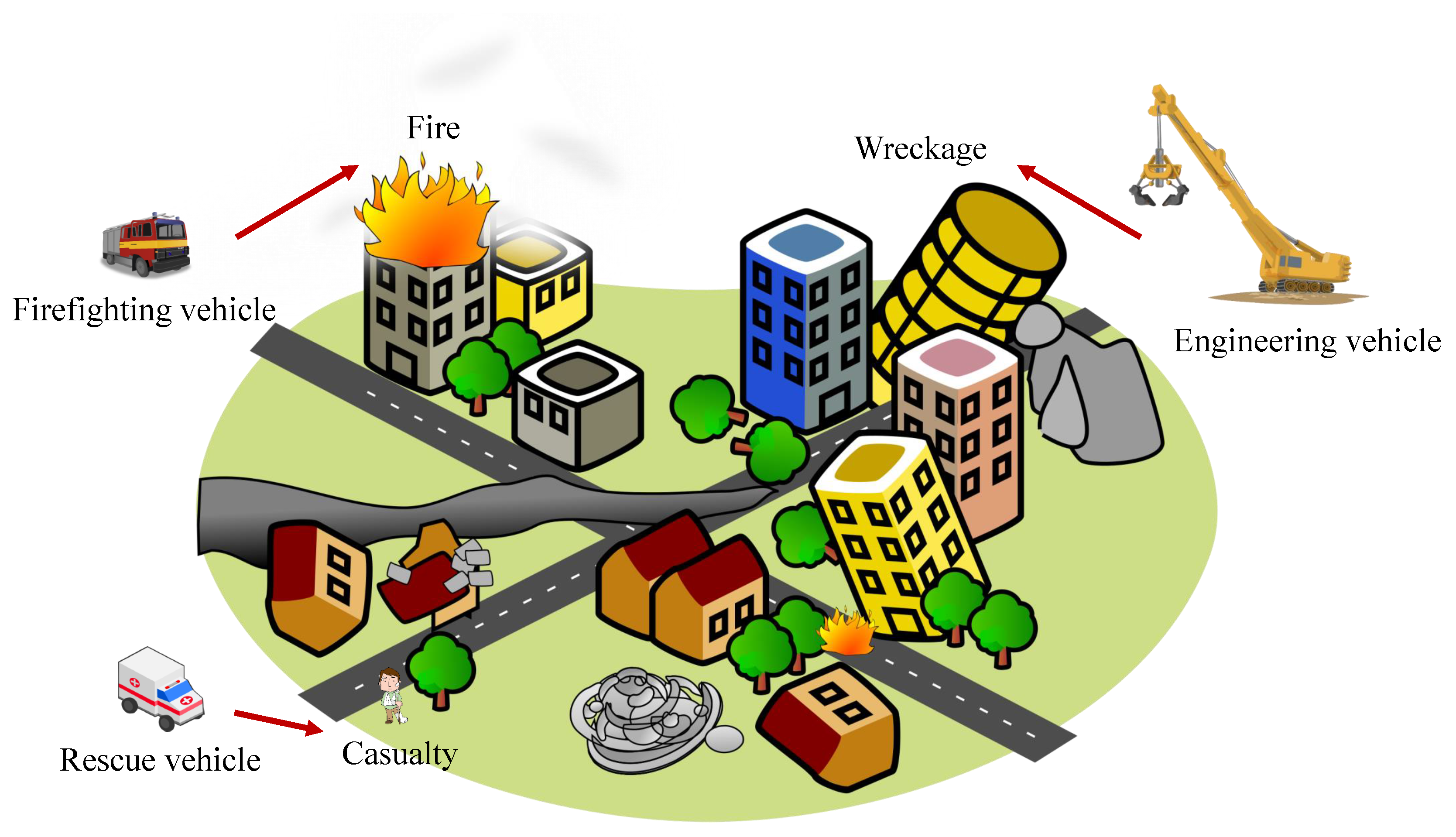
We assess the game design and equilibrium selection algorithm in a simulated disaster relief operation in a 10-by-10 grid world. In this operation, there are three types of mission-specific autonomous vehicles, each with varying response capabilities, to be allocated to different types of disaster situations. The engineering vehicles are capable of clearing wreckage from collapsed structures while the rescue vehicles are required to extract casualties to a safe location and the firefighting vehicles are equipped to deal with fire outbreaks in the region. The agent-task compatibilities are depicted in Figure 2. Furthermore, some sites may be struck with more than one type of disaster which will then require agents to work together albeit with some constraints.

5.1. Mission Coupled Constraints

• In an area where a fire broke out due to collapse of structures, cooperation of both engineering vehicles and firefighting vehicles will be required. To allow the engineering vehicles to begin clearing the wreckage efficiently, the fire needs to be first extinguished. Wreckage clearance task is dependent on the response to fire and must begin after the fire has been extinguished.
• In a fire outbreak, some casualties may be trapped in the fire. Assuming that the rescue vehicles are well-equipped to withstand some levels of heat such that casualty extraction is possible when firefighting vehicles are on site to provide assistance in controlling the fire. Furthermore, casualty extraction will not be possible after the fire has been extinguished as the casualties will have likely suffocated during the process of firefighting. Casualty rescue is dependent on firefighting operation and must begin during firefighting.
• The rescue vehicles do not possess the heavy lifting capabilities required to rescue casualties trapped in a wreckage. Assistance from the engineering units is required. Casualty rescue is dependent on wreckage clearance task and must begin after the wreckage have been cleared.

These constraints are only applicable when the tasks are in the same position (e.g., casualties trapped in a burning house.) The mission coupled constraints for these sites with multiple types of disaster can be reflected in the dependency matrix (

Table 3. Mission Dependency matrix.

	Fire	Casualty	Wreckage
Fire	0	1	1
Casualty	0	0	0
Wreckage	0	1	0

) and temporal matrix (

Table 4. Mission Temporal matrix.

	Fire	Casualty	Wreckage
Fire	0	4	3
Casualty	0	0	0
Wreckage	0	3	0

) as follows:

5.2. Feasibility of Game Model

Several agents and disaster sites at random locations of the grid world were considered. The summary of the disaster relief operations and agent parameters are provided in

Table 5. Disaster relief operation details and simulation parameters.

Agents	6	Tasks	27	Parameters
Engineer	2	Fire	3	Path length	4
Rescue	2	Casualty	3	Sample size	20
Firefighter	2	Wreckage	3	Confirmations	100
		Casualty $\stackrel{\mathrm{dep}}{\to }$ Fire	3	Hold period	4
		Casualty $\stackrel{\mathrm{dep}}{\to }$ Wreckage	3
		Wreckage $\stackrel{\mathrm{dep}}{\to }$ Fire	3

${}^{\stackrel{\mathrm{dep}}{\to }}$ depicts a dependency relationship (i.e., a task of each type in the same location leading to a coupled constraint).

with 20 different relief operations, each simulated as a game to be played 20 times each. The reward for the successful completion of each task was given as a time-decaying function

$$v_{k_j}\left(a\right)={\nu }_{k_j}exp(-{\lambda }_{k_j}{t}_{k_j}^c\left(a\right))$$

(20)

where ${\nu }_{k_j}$ is the intrinsic value of the task, and ${\lambda }_{k_j}$ is the discount factor for task $k_j$, to reflect the urgency of the tasks and motivate the agents to work in an efficient manner.

The feasibility of the game model using DSA with sampling can be inferred from the satisfaction of all coupled constraints in all the solutions obtained and the stochasticity of DSA is evident from the variation in global score values and computational times across the games for every operation scenario. For a centralized approach, the computational time for each game is below 1 min and when considering a synchronous decentralized approach, the estimated computational time falls to generally below 10 s. In a decentralized approach, each agent will run the scheduling algorithm, based on other agents’ previous actions, independently. After evaluating the possible schedules, the agent will decide on its choice of action and communicate its decision to all other agents. Without explicitly considering the means of communication but assuming synchronous, the simulation times of a decentralized approach is estimated based on the slowest agent for each iteration and the overheads accumulated in the communication process. For a synchronous decentralized approach, the model can provide a feasible solution quickly.

Figure 3 provides the graphical interpretation of a proposed schedule for one of the simulated games and information on the labels for the schedule are provided in

Table 6. Labeling information for agents and tasks.

Label	Type
A1, A2	Engineer
A3, A4	Rescue
A5, A6	Firefighter
1, 2, 3	Fire
4, 5, 6	Casualty
7, 8, 9	Wreckage
11$\stackrel{\mathrm{dep}}{\to }$10, 13$\stackrel{\mathrm{dep}}{\to }$12, 15$\stackrel{\mathrm{dep}}{\to }$14	Casualty $\stackrel{\mathrm{dep}}{\to }$ Fire
17$\stackrel{\mathrm{dep}}{\to }$16, 19$\stackrel{\mathrm{dep}}{\to }$18, 21$\stackrel{\mathrm{dep}}{\to }$20	Casualty $\stackrel{\mathrm{dep}}{\to }$ Wreckage
23$\stackrel{\mathrm{dep}}{\to }$22, 25$\stackrel{\mathrm{dep}}{\to }$24, 27$\stackrel{\mathrm{dep}}{\to }$26	Wreckage $\stackrel{\mathrm{dep}}{\to }$ Fire

.

The schedule in Figure 3 represents but one of many possible solutions to the simulated scenario. For a complex multi-agent multi-task allocation problem coupled with a flexible hold period, multiple Nash equilibria are likely to exist and the stochasticity of the agents’ actions due to random sampling leads to variation in the route of progression for each game, and thereby terminating at various different solutions. Regardless of the progression, the feasibility of the scheduling algorithm to satisfy the temporal constraints are evident from the complementary behaviors portrayed in the solution (e.g., A rescue-type agent (A4) waits at a casualty-type task (13) for a short period so that the temporal constraint which require the rescue (13) to occur during firefighting (12) can be satisfied, rescue-type agent (A4) attempts a casualty rescue (21) task after the wreckage (20) have been cleared by an engineer-type agent (A1), etc.)

Moving beyond providing a feasible solution, the game should converge within a reasonably short time period to ensure the practically of a game-theoretic implementation in real-world operations and hence, further studies on the number of confirmations $t_{\mathrm{con}}$ and sample size s, which are the main parameters influencing the rate of convergence, are presented in the subsequent sections.

5.3. Number of Confirmations

In this section, the effects of variation in number of confirmations on the global score and computation times are examined. Simulation of an operation setting similar to the example in Table 5 but with varying number of confirmations at 10, 50, 100, 500, and 1000, respectively, were considered and the results are shown in Figure 4 with the means and standard deviations for the various aspects of the simulation presented in

Table 7. Mean and standard deviation for global scores.

Confirmations	Mean	Standard Deviation
10	245.302	8.088
50	251.692	8.114
100	249.176	8.420
500	250.786	6.581
1000	251.295	6.556

,

Table 8. Mean and standard deviation for centralized computation times.

Confirmations	Mean	Standard Deviation
10	3.772	1.901
50	12.083	2.749
100	18.086	4.173
500	64.859	7.391
1000	120.583	5.699

and

Table 9. Mean and standard deviation for estimated decentralized computation times.

Confirmations	Mean	Standard Deviation
10	0.720	0.383
50	2.268	0.512
100	3.400	0.818
500	12.152	1.508
1000	22.410	1.063

. The observed global scores are generally similar at the selected levels of confirmations and the standard deviation generally decreases with increasing number of confirmations, providing a tighter bound to the range of scores. Intuitively, the decrease in standard deviation is in relation to the increasing probabilities of the solution being a Nash equilibrium (refer to Appendix A).

With only 10 confirmations, the mean global score is recognizably lower, and the range is also obviously greater as compared to the global scores for games with higher levels of confirmation. This lower levels of performance can be attributed to the extremity of the constraints placed on the agents’ action set. With a sample size of 20 and 10 confirmations, the agents are expected to be exposed to a maximum of 191 unique actions which barely covers approximately 5% of all possible actions. The exposure of an agent refers to the number of actions that it has seen from the moment when it last changed its action. As such, it is plausible that the agents do not have sufficient understanding of the full range of possible actions, leading to agreements that are less efficient. However, it should be noted that such inefficiencies lead to a global score which is merely 3% lower as seen in Figure 5. Indeed, it can be argued that agents do not need to understand the entirety of their action sets to arrive at reasonable solutions. With 50 confirmations, the maximum exposure is at 951 unique actions, or approximately 26% of all possible actions. Yet, mean global scores comparable to those at higher levels of exposure are observed. With 1000 confirmations, it is highly likely that every agent has seen its entire possible action set since there are only 3610 possible actions while it is exposed to 19,001 non-unique actions. Interestingly, the maximum scores achieved for each category are similar with a value of 259.862 except for simulations with only 10 confirmations having a slightly lower maximum of 259.791. This phenomenon will be amplified in dense task allocation settings since most tasks will be closely grouped together and most action sequences will provide similar levels of reward. As such, most Nash equilibria will provide near-optimal solutions and it is, therefore, unnecessary for agents to have a complete understanding of their possible actions since emphasis is not placed on achieving the solution with an optimal global score or the Nash equilibrium with the maximum global score. When constraints are provided at every iteration, agents have lesser numbers of choices to make at each iteration, allowing them to arrive at a general agreement more quickly and easily as evident in the short computation times for games with only 10 confirmations. Improvements to the agreement are then made as the agents continue to explore the possible action space for each iteration.

However, it is necessary to note that increasing the confirmations do not necessarily lead to increase in global scores for every play. Recall that in DSA, progression is stochastic and hence the Nash equilibrium obtained for every play may differ and therefore, there is a non-zero probability of reaching a Nash equilibrium that has the lowest possible score despite considering a high number of confirmations in one play while having a Nash solution with a higher score when considering lower number of confirmations.

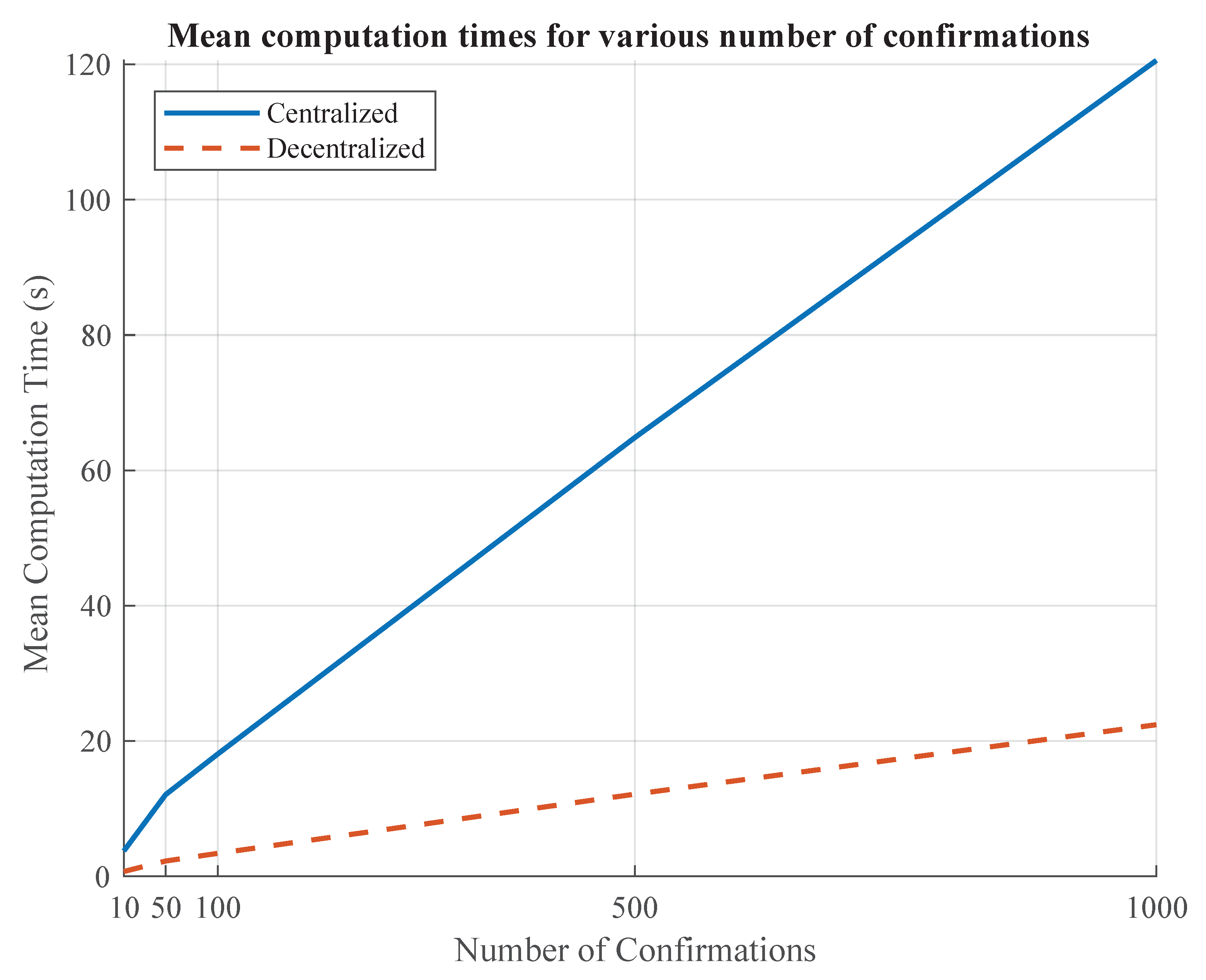
Another observation made, from Figure 6, is that the computation times increase with the number of confirmations as expected. In essence, a confirmation is defined as an iteration where all agents do not change their actions. This also means that in the new constrained action set of any agent at the current iteration, there are no actions that can improve any agent’s local utility. For $t_{\mathrm{con}}$ confirmations, all agents do not change their actions for $t_{\mathrm{con}}$ consecutive iterations. When the agreement between the agents is not a Nash equilibrium, then the possibility of such an event occurring decreases with increasing values of $t_{\mathrm{con}}$. Therefore, as the number of confirmations increases, confidence on the solution being Nash increases, but at the expense of increasing computation time due to the additional evaluations made by the agents.

5.4. Size of Samples

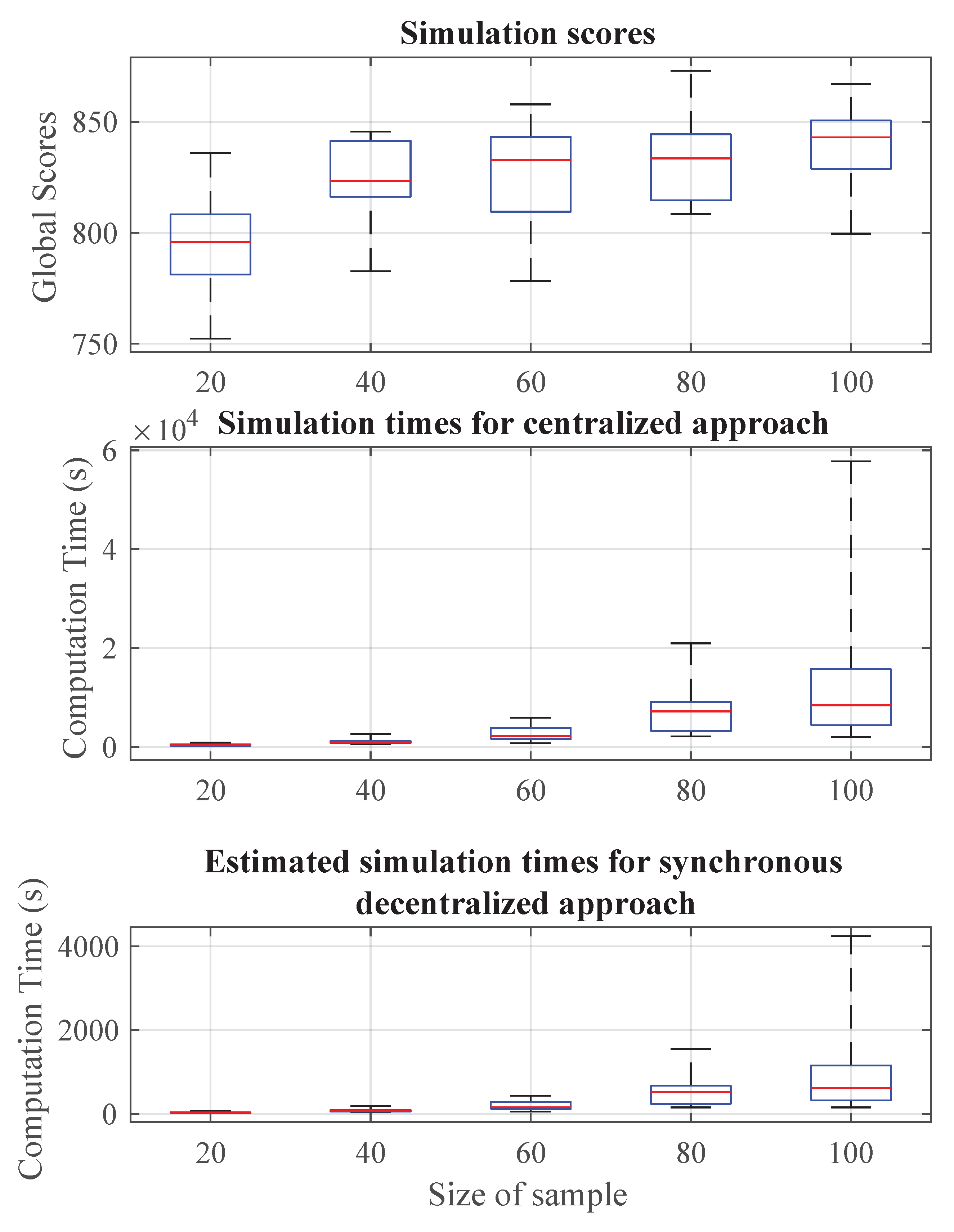
To investigate the impact of variation in sample size, a dense allocation setting given in

Table 10. Crowded disaster relief operation details and simulation parameters.

Agents	15	Tasks	90	Parameters
Engineer	5	Fire	10	Path length	4
Rescue	5	Casualty	10	Confirmations	100
Firefighter	5	Wreckage	10	Hold period	4
		Casualty $\stackrel{\mathrm{dep}}{\to }$ Fire	10
		Casualty $\stackrel{\mathrm{dep}}{\to }$ Wreckage	10
		Wreckage $\stackrel{\mathrm{dep}}{\to }$ Fire	10

is considered. The world remains as a 10-by-10 grid but the number of agents and tasks increased significantly and the sample sizes were varied to be 20, 40, 60, 80, and 100. The simulation results for the dense task allocation game are displayed in Figure 7,

Table 11. Mean and standard deviation for global scores.

Sample Size	Mean	Standard Deviation
20	795.294	21.166
40	823.923	16.742
60	825.086	21.365
80	831.913	17.918
100	839.281	18.486

,

Table 12. Mean and standard deviation for centralized computation times.

Sample Size	Mean	Standard Deviation
20	404.854	165.431
40	1093.975	476.654
60	2804.496	1593.538
80	7360.438	5086.329
100	12,632.142	12,861.328

and

Table 13. Mean and standard deviation for estimated decentralized computation times.

Sample Size	Mean	Standard Deviation
20	30.295	12.386
40	80.517	35.030
60	205.754	116.449
80	542.142	376.058
100	928.077	944.542

.

Predictably, the mean global score values increase with increasing size of sample. The sample sizes of 20, 40, 60, 80, and 100 provided each agent with exposure to approximately 0.3%, 0.6%, 0.9%, 1.2% and 1.4% of its entire action set, respectively. Such low levels of understanding of the action set usually means that the agreements are suboptimal since the probability of making improvements to the existing agreement is rather high. Despite the suboptimality of the solutions, it should be noted that a 5-fold increase in sample size from 20 to 100 led to improvements in score by a mere 5% as seen in Figure 8. The logarithmic increment trend for the global scores further supports our belief that agents can make reasonably good scheduling decisions despite having an incomplete, and possibly small, understanding of their action set in a dense task allocation setting.

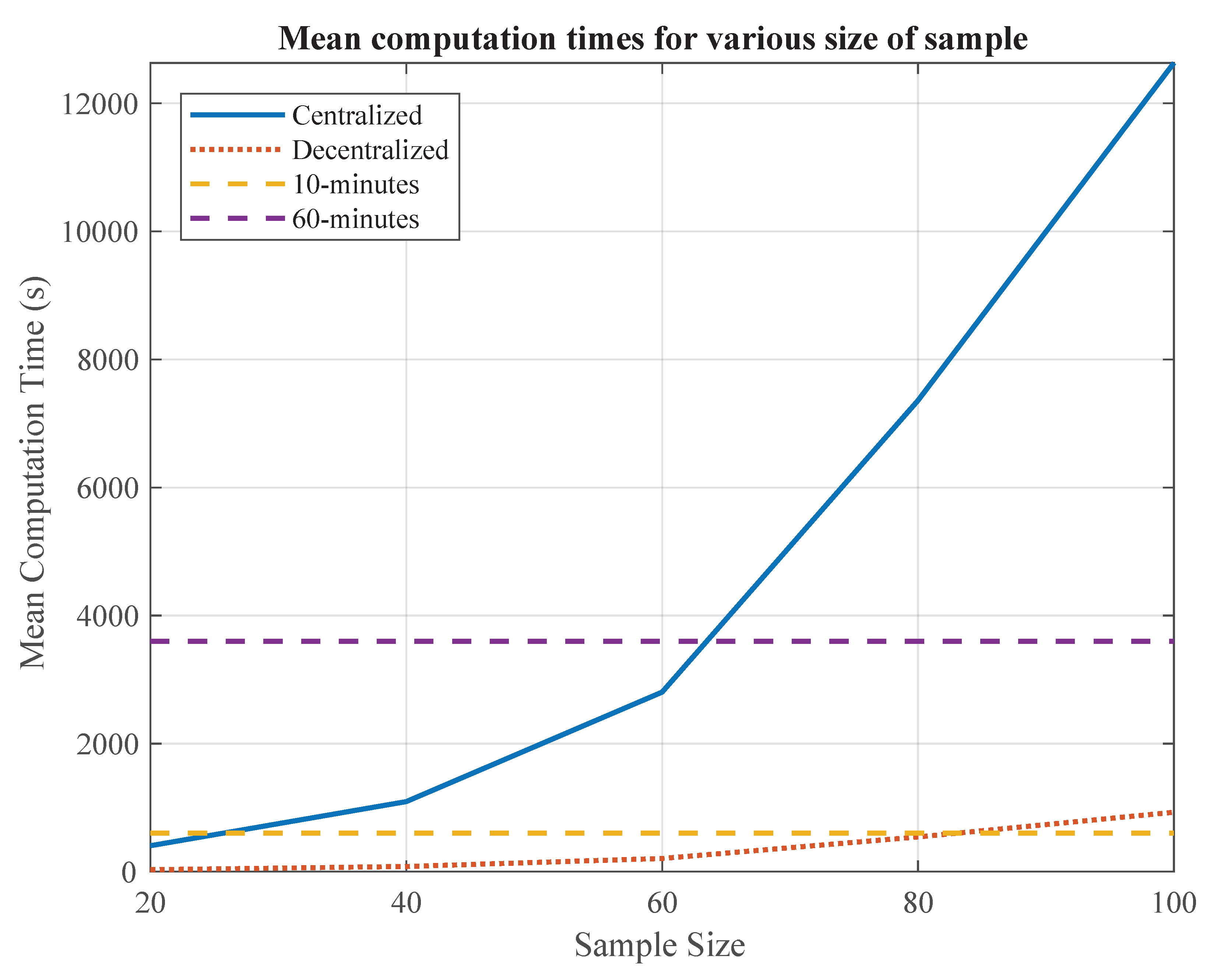
More importantly, from Figure 9, the computation times were observed to increase exponentially with the sample size. Without the use of sampling in the equilibrium selection, a game-theoretic approach for task allocation in a dense emergency operation will simply be impractical. Using random sampling, the computation times were suppressed to provide reasonably good solutions, enabling game-theoretic implementations in emergency operations which tend to be crowded, complex, and time-sensitive. In the game simulated, the mean computation times for both the centralized and decentralized approach were kept well below 60 min and 10 min, respectively, when the sample sizes are kept smaller than 60. Feasibly good solutions were also obtained quickly when considering a sample size of only 20 in the simulations.

6. Conclusions

In this paper, we introduced a game-theoretic framework for allocation of tasks with spatial and temporal coupled constraints first seen in CCBBA. A game-theoretic modeling of such problems helps to overcome potential convergence issues faced in a market-based allocation model through leveraging on the properties of potential games. A well-designed game model alone can effectively overcome spatial relationships among tasks and when coupled with the scheduling algorithm, allows feasible assignment of tasks with both spatial and temporal dependencies. Additionally, existing equilibrium selection algorithms have commonly been restricted by the size of the problem, making implementation of game-theoretic theoretic task allocation impractical for large-scale problems. However, by using random sampling in DSA, it is possible to obtain a feasibly good solution within a short time, allowing game-theoretic implementations in emergency operations which frequently consist of large numbers of tasks with complex relationships and yet require quick allocation at the same time.

The greatest limitation for the proposed methodology lies in the inability to quantify or guarantee the optimality of any given solution, in terms of global allocation, despite its feasibility to provide an allocation solution that considers the spatial and temporal relationships between the different types of task. A plausible explanation may be due to the existence of multiple Nash equilibria and the probabilistic approach in DSA. Additional studies to limit the game model to have only a single Nash equilibrium or to consider deterministic equilibrium selection algorithms that are a capable of selecting the Nash equilibrium with the maximum global allocation scores will help to overcome this deficiency.

Despite the current flaws in the proposed methodology, reasonably good solutions can still be obtained quickly to tackle coupled-constraint task allocation problem in a crowded space.

References

- Arslan, G.; Marden, J.R.; Shamma, J.S. Autonomous vehicle-target assignment: A game-theoretical formulation. J. Dyn. Syst. Meas. Control 2007, 129, 584–596. [Google Scholar] [CrossRef]
- Chapman, A.C.; Micillo, R.A.; Kota, R.; Jennings, N.R. Decentralised dynamic task allocation: A practical game: Theoretic approach. In Proceedings of the 8th International Conference on Autonomous Agents and Multiagent Systems, Budapest, Hungary, 10–15 May 2009; Volume 2, pp. 915–922. [Google Scholar]
- Choi, H.L.; Brunet, L.; How, J.P. Consensus-based decentralized auctions for robust task allocation. IEEE Trans. Robot. 2009, 25, 912–926. [Google Scholar] [CrossRef]
- Gerkey, B.P.; Mataric, M.J. Sold!: Auction methods for multirobot coordination. IEEE Trans. Robot. Autom. 2002, 18, 758–768. [Google Scholar] [CrossRef]
- Li, N.; Marden, J.R. Designing games to handle coupled constraints. In Proceedings of the 49th IEEE Conference on Decision and Control (CDC), Atlanta, GA, USA, 15–17 December 2010; pp. 250–255. [Google Scholar]
- Li, N.; Marden, J.R. Decoupling coupled constraints through utility design. IEEE Trans. Autom. Control 2014, 59, 2289–2294. [Google Scholar] [CrossRef]
- Parker, L.E.; Tang, F. Building multirobot coalitions through automated task solution synthesis. Proc. IEEE 2006, 94, 1289–1305. [Google Scholar] [CrossRef]
- Whitten, A.K.; Choi, H.L.; Johnson, L.B.; How, J.P. Decentralized task allocation with coupled constraints in complex missions. In Proceedings of the 2011 American Control Conference, San Francisco, CA, USA, 29 June–1 July 2011. [Google Scholar]
- Netto, R.; Ramalho, G.; Bonatto, B.; Carpinteiro, O.; Zambroni de Souza, A.; Oliveira, D.; Braga, R. Real-Time Framework for Energy Management System of a Smart Microgrid Using Multiagent Systems. Energies 2018, 11, 656. [Google Scholar] [CrossRef]
- Han, Q.; Tan, G.; Fu, X.; Mei, Y.; Yang, Z. Water resource optimal allocation based on multi-agent game theory of HanJiang river basin. Water 2018, 10, 1184. [Google Scholar] [CrossRef]
- Baldoni, M.; Baroglio, C.; May, K.M.; Micalizio, R.; Tedeschi, S. Computational Accountability in MAS Organizations with ADOPT. Appl. Sci. 2018, 8, 489. [Google Scholar] [CrossRef]
- Marden, J.R.; Arslan, G.; Shamma, J.S. Joint strategy fictitious play with inertia for potential games. IEEE Trans. Autom. Control 2009, 54, 208–220. [Google Scholar] [CrossRef]
- Bowling, M.; Veloso, M. An Analysis of Stochastic Game Theory for Multiagent Reinforcement Learning; Technical Report; Carnegie-Mellon Univ Pittsburgh Pa School of Computer Science: Pittsburgh, PA, USA, 2000. [Google Scholar]
- Heinrich, J.; Silver, D. Deep reinforcement learning from self-play in imperfect-information games. arXiv 2016, arXiv:1603.01121. [Google Scholar]
- Wang, Y.; Pavel, L. A Modified Q-Learning Algorithm for Potential Games. IFAC Proc. Volumes 2014, 47, 8710–8718. [Google Scholar] [CrossRef] [Green Version]
- Lim, M.C.; Choi, H.L. A Game-Theoretic Approach for Multi-Robot Task Allocation with Dependency Constraints. In Proceedings of the 5th International Conference of Robot Intelligence Technology and Applications, Daejeon, Korea, 13–15 December 2017. [Google Scholar]
- Monderer, D.; Shapley, L.S. Potential games. Games Econ. Behav. 1996, 14, 124–143. [Google Scholar] [CrossRef]
- Chapman, A.; Rogers, A.; Jennings, N.R. A Parameterisation of Algorithms for Distributed Constraint Optimisation via Potential Games. 2008. Available online: https://eprints.soton.ac.uk/265208/ (accessed on 5 December 2016).
- Lã, Q.D.; Chew, Y.H.; Soong, B.H. Potential Game Theory: Applications in Radio Resource Allocation; Springer: Berlin, Germany, 2016. [Google Scholar]
- Marden, J.R.; Arslan, G.; Shamma, J.S. Cooperative control and potential games. IEEE Trans. Syst. Man Cybern. Part B Cybern. 2009, 39, 1393–1407. [Google Scholar] [CrossRef] [PubMed]
- Choi, H.L.; Lee, S.J. A potential game approach for information-maximizing cooperative planning of sensor networks. IEEE Trans. Control Syst. Technol. 2015, 23, 2326–2335. [Google Scholar] [CrossRef]
- Macarthur, K.S.; Stranders, R.; Ramchurn, S.D.; Jennings, N.R. A Distributed Anytime Algorithm for Dynamic Task Allocation in Multi-Agent Systems. In Proceedings of the Twenty-Fifth AAAI Conference on Artificial Intelligence, San Francisco, CA, USA, 7–11 August 2011; pp. 701–706. [Google Scholar]
- Lim, M.C. A Game-Theoretic Approach for Coupled-Constraint Task Allocation. Master’s Thesis, Korea Advanced Institute of Science and Technology, Daejeon, Korea, 2018. [Google Scholar]
- Chapman, A.C.; Rogers, A.; Jennings, N.R. Benchmarking hybrid algorithms for distributed constraint optimisation games. Auton. Agents Multi-Agent Syst. 2011, 22, 385–414. [Google Scholar] [CrossRef]
- Garivier, A.; Kaufmann, E.; Koolen, W.M. Maximin action identification: A new bandit framework for games. In Proceedings of the Conference on Learning Theory, New York, NY, USA, 23–26 June 2016; pp. 1028–1050. [Google Scholar]
- Marden, J.R.; Shamma, J.S. Revisiting log-linear learning: Asynchrony, completeness and payoff-based implementation. Games Econ. Behav. 2012, 75, 788–808. [Google Scholar] [CrossRef] [Green Version]
- Borowski, H.; Marden, J.R.; Frew, E.W. Fast convergence in semi-anonymous potential games. In Proceedings of the IEEE 52nd Annual Conference on Decision and Control, Florence, Italy, 10–13 December 2013; pp. 2418–2423. [Google Scholar]
- Tumer, K.; Agogino, A.K.; Wolpert, D.H. Learning sequences of actions in collectives of autonomous agents. In Proceedings of the First International Joint Conference on Autonomous Agents and Multiagent Systems: Part 1, Bologna, Italy, 15–19 July 2002; pp. 378–385. [Google Scholar]
- Tumer, K.; Wolpert, D. A survey of collectives. In Collectives and the Design of Complex Systems; Springer: Berlin, Germany, 2004; pp. 1–42. [Google Scholar]
- Juhele. City after Earthquake [PNG File]. 2016. Available online: https://openclipart.org/detail/250253/city-after-earthquake (accessed on 23 February 2019).
- Markacio. Construction Crane [PNG File]. 2012. Available online: https://openclipart.org/detail/168285/construction-crane (accessed on 23 February 2019).
- Rdevries. Fire Truck [PNG File]. 2014. Available online: https://openclipart.org/detail/190874/fire-truck (accessed on 23 February 2019).
- Ginkgo. Isometric Ambulance [PNG File]. 2016. Available online: https://openclipart.org/detail/252628/isometric-ambulance (accessed on 23 February 2019).
- Oksmith. Injured [PNG File]. 2017. Available online: https://openclipart.org/detail/285043/injured (accessed on 23 February 2019).
Figure 1.
Decomposition of between coupled constraint.
Figure 2.
Agent-Task compatibilities in a disaster relief operation [30,31,32,33,34]. The figure is a composite image constructed from the various sources cited.
Figure 3.
Example of a feasible schedule.
Figure 4.
Variations in global scores and computation times due to number of confirmations.
Figure 5.
Mean global score values for various number of confirmations.
Figure 6.
Mean computation times for various number of confirmations.
Figure 7.
Variations in global scores and computation times due to size of sample.
Figure 8.
Mean global score values for various sample sizes.
Figure 9.
Mean computation times for various sample sizes.