Evaluation of Calf Muscle Reflex Control in the ‘Ankle Strategy’ during Upright Standing Push-Recovery

1
Intelligent System Research Institute, School of Automation, Wuhan University of Technology, Wuhan 430070, China
2
Intelligent System & Biomedical Robotics Group, School of Computing, University of Portsmouth, Portsmouth PO1 3HE, UK
*
Author to whom correspondence should be addressed.
Appl. Sci. 2019, 9(10), 2085; https://doi.org/10.3390/app9102085
Submission received: 28 February 2019
/
Revised: 16 May 2019
/
Accepted: 16 May 2019
/
Published: 21 May 2019
(This article belongs to the Special Issue Human Friendly Robotics)
Abstract
:Featured Application
Robotic device control and Human movement studying.
Abstract
Revealing human internal control mechanisms during environmental interaction remains paramount and helpful in solving issues related to human-robot interaction. Muscle reflexes, which can directly and rapidly modify the dynamic behavior of joints, are the fundamental control loops of the Central Nervous System. This study investigates the calf muscle reflex control in the “ankle strategy” for human push-recovery movement. A time-increasing searching method is proposed to evaluate the feasibility of the reflex model in terms of predicting real muscle activations. Constraints with physiological implications are imposed to find the appropriate reflex gains. The experimental results show that the reflex model fits over 90% of the forepart of muscle activation. With the increasing of time, the Variance Accounted For (VAF) values drop to below 80% and reflex gains lose the physiology meaning. By dividing the muscle activation into two parts, the reflex formula is still workable for the rest part, with different gains and lower VAF values. This result may indicate that reflex control could more likely dominate the forepart of the push-recovery motion and an analogous control mechanism is still feasible for the rest of the motion part, with different gains. The proposed method provides an alternative way to obtain the human internal control mechanism desired for human-robot interaction task.
1. Introduction
Human-robot interaction, especially physical interaction, has recently drawn great and increasing attention [1]. Many wearable ankle joint robotic devices and control methods have been developed to enhance human locomotion ability [2,3]. For robot-assisted implementation, it is suggested that robot devices should not override human control, but rather involve the user in the control [4]. One key challenge is that traditional path and trajectory planning for robots may be unfeasible, since it is difficult for robots to know the human motion beforehand. Revealing the human internal control mechanism facing the physical interaction task shows an alternative way to provide a reference for robotic control system design [5].
Joint-level response to physical interaction with humans is unique to present-day robotic systems, in which central control and stiff joint are widely adopted. Despite having achieved great breakthroughs in whole-body control of robots in different tasks, it depends heavily on high-accuracy sensation, and is computationally expensive, resulting in robot multiple-joint control remaining difficult and challenging [6]. The human joint is not completely governed by the brain, and is not as stiff as those of most robots. There are local self-responses in joints to external disturbances, especially in the case of sudden situations. Investigating the joint-level properties of humans is not only physiologically meaningful, but also beneficial to the establishment of highly efficient robotic systems.
Muscle reflexes, which enhance the active response of muscles to disturbances, influence dynamic muscle properties and contribute to muscle tension adjustment, are located on the fundamental lower layer of the Human Central Nervous System [7]. The shortest control loop makes muscle reflexes the first active response to unexpected external disturbance. Some researchers deem reflexes to be essential to many everyday human activities, such as quiet standing [8]. Modulating ankle extensors may be affected by body sway velocity during quiet standing [9], indicating that body velocity is one of the most important inputs in reflex control loops. Under strong disturbances, feed-forward mechanisms modified by the cortex may be involved [10]. The experimental environment has to be strictly controlled in order to focus on muscle reflexes as much as possible [11].
Investigating the control model of human muscle reflexes can provide insights into the fundamental principles governing human locomotion. The muscle spindle is sensitive to change in muscle fiber length, as well as the rate of the change. When the muscle is stretched, the spindle first generates bio-electrical signals, which are transmitted to the spinal cord. Afterwards, the spinal cord produces feedback signals to activate muscle fibers, so that the muscle fibers contract against the stretch. A proportional and derivative (PD) model is usually used to represent this process [12]. Prochazka et al. [13] suggest that a positive force feedback needs to be considered. Combined with interneuron delay and muscle biomechanical properties, the positive force feedback loop can provide stable force compensation [14].
One of the challenges in the investigation of muscle reflex is to evaluate the feasibility of the proposed model. As the output of the muscle reflex loop, electromyography signals (EMG) provides a convenient means of model evaluation. Surface EMG (sEMG) is a noninvasive technology that is widely used in the clinic [15,16,17] and in engineering study [18,19,20,21]. As sEMG signals are sensitive to noises, they are merely used as monitor signals in some studies [12]. Also, sEMG signals can be implemented to predict muscle tendon force [22] or control robotic devices [23], as long as they are properly processed, usually transformed to muscle activation level. Furthermore, a musculoskeletal model [24,25,26] is often integrated with sEMG signals to obtain accurate prediction results. The calculated muscle activation is usually used to evaluate the feasibility of the proposed model. Lockhart and Ting [27] propose a second-order feedback model to interpret muscle activation patterns with respect to a sudden loss of balance in cats. Interestingly, the mathematical form of the second-order model proposed by Lockhart and Ting is the same as the summation of the stretch reflex and positive force feedback models [14]. Also, the variables in the model proposed by Lockhart and Ting include the acceleration, velocity and position of Center of Mass (CoM). The corresponding results proposed by Ting seem to be more like a higher control strategy, while the muscle reflex studied in this paper is a local response mechanism.
Apart from the potential advantage of investigating muscle reflex, as noted above, the implementation of muscle reflex can also suggest some valuable clues for solving human-robot interaction problems. Geyer and Herr [28] proposed some simplified muscle reflex pathways to establish a human walking controller under a MATLAB simulation environment. Distinct from the feed-forward gait generation method, which mainly depends on the estimation of CoM and CoP, only muscle reflexes presented by Geyer and Herr (feedbacks from proprioception of different joints and positive force self-excitation) are implemented to generate the locomotion pattern. By using optimized parameters, the walking controller proposed by Geyer and Herr has shown the potential to achieve human-like walking and self-stability against disturbances in a simulation study. Thatte and Geyer [29], in the following study, applied a similar neuromuscular model with muscle reflex control on leg prostheses, to fulfill balance recovery. This muscle reflex-based controller is also capable of controlling a bipedal robot [30].
The human ankle joint contacts the ground directly and plays an important role in upright standing. A simple spring-like model was assumed by Winter et al. [31] for ankle muscle control during quiet standing. In their model, the human body was presumed to be an inverted pendulum (IP), swaying around the ankle joint. The ankle joint acted like a torsional spring to maintain body quiet standing balance. This type of spring-like behavior was considered to be due to the controlling results from Central Nervous System (CNS). To investigate the internal quiet standing control mechanism, based on a similar IP model to that suggested by Winter, Masani et al. [32] applied a PD controller to yield the preceding motor commands. However, there are few studies evaluating the reflex mechanism in dynamic push-recovery upright standing, in which a disturbance is imposed.
Although many ankle joint robots have been designed to enhance human locomotion ability, little attention has been paid to assisting upright standing balance with ankle joint exoskeletons [33]. To achieve this goal, understanding the human ankle joint-level internal control mechanisms such as reflex control under push-recovery situations is important. Although a considerable amount of effort has been made in investigating upright standing, much of the research has been focused on the role of central control, i.e., examining the relation between CoM and human response. Further details from the point of view of the joint level are still needed to provide more direct guidelines for robot controller design. This paper evaluates the local reflex response of calf muscles and the corresponding ankle joint torque production during upright standing feet-in-place push-recovery. The aim of this study is twofold: (a) to investigating the human ankle joint reflex control mechanism facing sudden limited external disturbance, (b) to provide a fast method of using sEMG signals to calculate reflex control parameters and ankle joint torque. To explore reflex control, a time-increasing search method is applied to find a feasible time interval for reflex control. A two-piecewise response is revealed by the experimental results, and different gains seem to be adopted by subjects in the two-piecewise intervals.
The remainder of this paper is organized as follows. The muscle reflex, musculoskeletal system modeling and experimental setup are stated in Section 2. The experimental results are shown in Section 3. Section 4 ends this paper by the analysis and discussion of the experimental results, as well as showing several related issues.
2. Materials and Methods
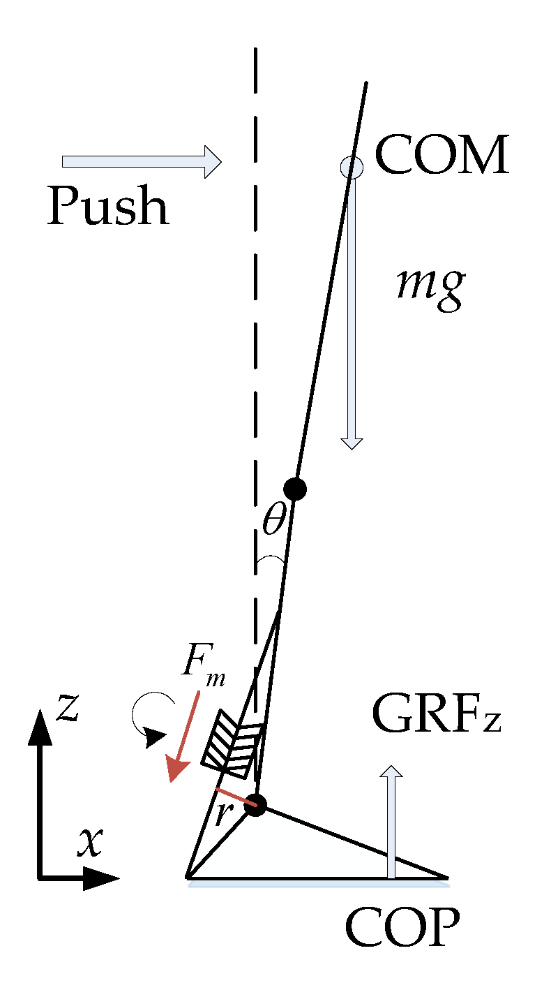
Upright standing push-recovery is depicted in a general way in Figure 1. The single IP model is usually adopted to describe the body dynamics. However, a multi-joint IP model is more applicable, as human joints are flexible when in a natural upright standing posture [34,35]. Thus, the body is not specifically assumed to be a single IP in this paper. Here, it is important to note that no matter which model is adopted, ankle joint torque is provided by the calf muscle. When subjected to external disturbance, the human body leans forward and loses its balance. In such cases, sensed by muscle sensory organs, the calf muscles are stretched and evoke a reflex response, so that resistant tendon force (Fm) can be produced to resist the external disturbance and balance the human body. As the reflex loop is short and fast, ankle joint torque is promptly provided to maintain the body’s upright balance.
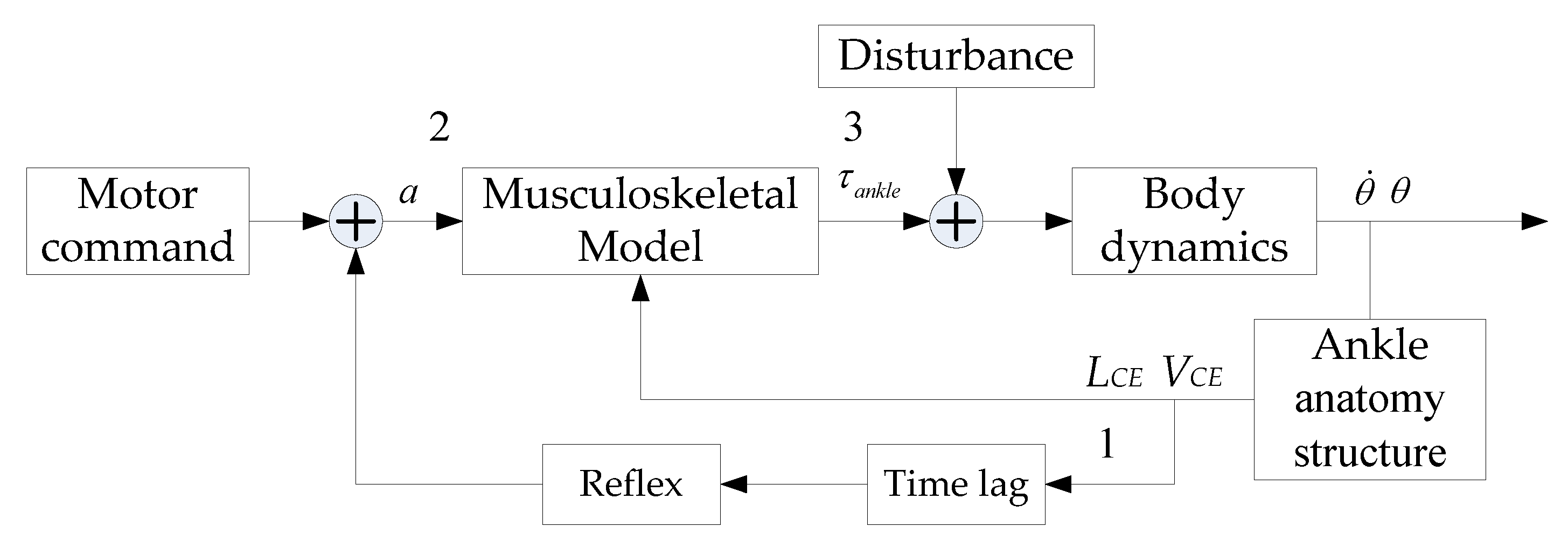
Based on the work of Fitzpatrick [36], the ankle joint neural-muscular control model is visualized in Figure 2, where a and τankle denote the muscle activation level and ankle joint torque, respectively. Disturbance stands for the external force exerted on the subject’s back. The musculoskeletal model includes a Hill-type muscular model and the muscle-skeleton anatomy structure. Information on the muscle movement arm (r) can be obtained from the anatomy structure. ‘Time lag’ contains the reflex pathway and the muscle dynamic time lag. The ‘motor command’ comes from the high level of the nervous system. As displayed in Figure 2, this study divides the ankle joint neural-muscular control model into two parts, that is, the reflex control part (from 1 to 2) and the ankle joint torque generation part (from 2 to 3). The reflex control part not only describes the way that the muscle activation is controlled by the muscle reflex, but also calculates the reflex gains. The ankle joint torque generation part depicts the manner in which muscle activation controls ankle joint torque and aims to figure out the relationship between muscle activation and ankle joint torque. Here, it is notable that muscle activation connects the aforementioned two parts.
2.1. Calf Muscle Reflex Model and Parameter Calculation
In this paper, the following muscle reflex model is adopted:
where p and d are, respectively, the gains for muscle spindle length change and the rate of the change in length. LCE0 indicates the optimal fiber length. a0 denotes the initial activation level. LCE is the current fiber length. VCE is the current rate of change of the fiber length, obtained from the first differentiation of LCE–LCE0. t0 represents the combined time delay caused by neural transmission and muscle electromechanical delays.
Recent research has demonstrated that the muscle spindle primary afferents in passive muscle fire in direct relationship to muscle force-related variables [37]. We assume that there is no conflict between Equation (1) and the force sensing function. The parameters p and d can be alternatively regarded as stiffness and damping, and they connect force information with the deformation of the muscle fibers. A detailed discussion can be found in Section 4.2.
Based on the discovery noted in [38], the length of calf fibers increases linearly with the ankle joint angle in the range of the experiment. Thus, LCE is simplified as:
where cl represents this linear relationship.
Substituting Equation (2) into Equation (1), the following equation is obtained:
For simplicity and without loss of generality, pc and dc are, respectively, represented by pa and da in the rest of this study.
It is appropriate to add an acceleration item in Equation (1), as acceleration has been proved to be useful and important in the literature. However, the results are not significantly improved in our experiment condition. A further discussion can be found in Section 4.1.
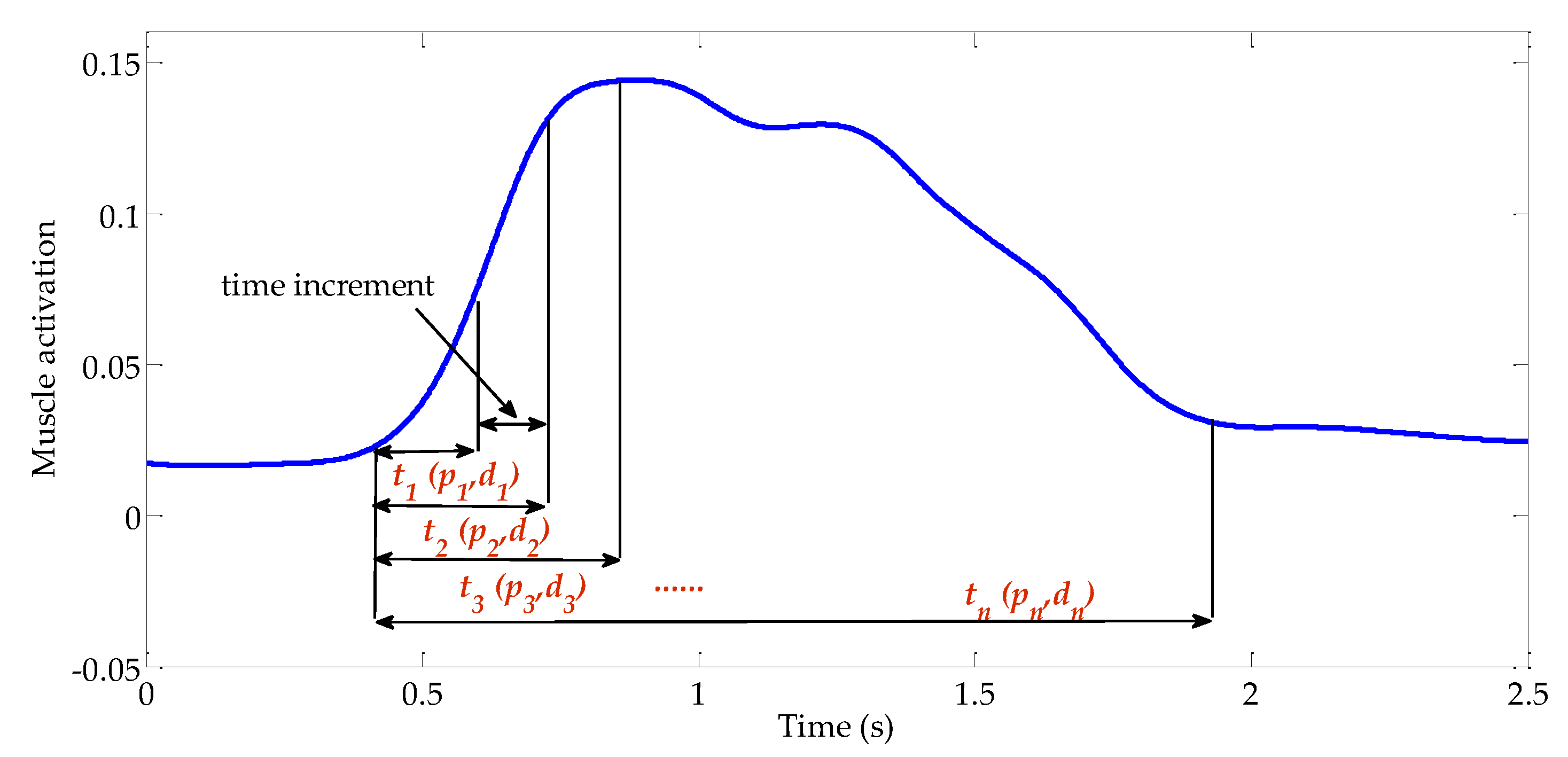
Data (a, θ and ) recorded from experiments are used to calculate pa and da. As high-level command may be involved in the control process, it is uncertain what length of time interval is most appropriate to be used. A time-increasing searching method, as illustrated in Figure 3, is proposed to find a proper time interval. The start-point of the time interval is at the time point where angular velocity begins to increase. The threshold of angular velocity is empirically set to be 0.01 rad/s. The end-point moves from the start-point to the end-point, at which muscle activation returns to the normal level with a time increment of 10 ms.
pa and da are calculated by data (a, θ and ) recorded from experiments using a simple linear regress algorithm. The input is X (X = [θ 1]T) and the output is a. The parameter vector (w = [pa da a0]) is calculated by (XTX)−1XTa. pa and da are calculated at each time increment. As a result, a set of (pa, da) pairs is obtained. The Variance Accounted For (VAF) between the prediction and recorded muscle activation levels is used to evaluate the proper time point as follows:
where var and â stand for the variance and the prediction value, respectively. VAF is calculated at each time increment. According to the meaning of stretch reflex, pa and da should be positive. This physiological constraint is added to find appropriate values of pa and da.
2.2. Muscle Activation Calculation
The muscle activation level (a) is obtained from raw sEMG signals and can be calculated by the method recommended by Buchanan et al. [39]. The filters used in this paper are all 4th-order zero-lag shift Butterworth filters having different types and cutoff frequencies. The raw sEMG signals are first passed through a high-pass filter with a cutoff frequency of 5 Hz to remove the DC offsets. Then, they are rectified and passed through a low-pass filter with a cutoff frequency of 3 Hz. This process is implemented to mimic the low-pass effect of muscle force generation characteristic and obtain a smooth trend. For a further analysis of the low-pass cutoff frequency, the reader is referred to the discussion section of this paper. The filtered signal denoted by e(t) is normalized using the maximum voluntary contraction (MVC) test activation value. a(t) is then calculated as follows [39]:
Equation (5) represents the muscle activation dynamics. Equation (6) is used to de-linearize the results. In this paper, parameters α, β1, β2 and A are set as 2.25, 1, 0.25 and −0.5, respectively. The effects of different low cutoff frequencies are also tested in discussion section. The lower the low-pass cutoff frequency is, the smoother the activation level will be. A smooth result can be more suitable for engineering applications, although it may suffer from the deficiency that some valid signal may be eliminated in clinic analysis.
2.3. Hill-Type-Based Muscular Model
Calf muscle is activated by activation stimulation and contracts to produce tension or muscle force (FM). The ankle joint torque is predicted by the summation of tensions of the calf muscle tendon units (MTUs). The Hill-type muscular model is implemented to calculate Fm. The conventional form described in [22] is adopted. There are two main parts, namely, the passive serial element (SE) and the contractile element (CE) parts. The SE part represents the elastic property of the muscle tendon. The CE part is composed of a contractile element (CE) and a passive element (PE). PE represents the muscle fiber passive force property. As a passive stiffness part is added in SE, PE is ignored in the calculation. The muscle fore, FM, can be calculated as follows:
where FPE and FCE are the passive and active force generated by muscle fiber, respectively. Fmax is the maximum muscle fiber force exerted at the optimal fiber length LCE0. VCE0 is the maximum rate of change of the muscle fiber length. θp and θp0 are, respectively, current and initial pennation angles. The equation for calculating θp is derived based on the assumption that the thickness and the volume of the muscle are constant. Due to the small change of ankle joint angle in this study, θp can be regarded as a constant. The initial parameter values of Fmax, LCE0, VCE0 and θp0 are based on those reported in [40]. Prior to using these parameters, they are scaled by the weight and height of the subject. In this study, it is assumed that that the fiber length is located at its optimum during quiet standing. Based on the assumption mentioned here, Fm is the maximum value at the same muscle activation level. Under such a condition, the human metabolic energy consumption can be minimized in order to maintain upright balance [41]. This means that the initial value of LCE is assumed to be the optimal length LCE0 in the calibration. Moment arm (r) is gained from a general model depicted in [40] and linearly scaled by the subject’s height. As the ankle joint angle changes within a small range, r is set to be a constant value. The Covariance Matrix Adaptation–Evolution Strategy (CMA-ES) optimization method adopted in [42] is implemented to find the proper parameters of the muscular model. The measured ankle joint torque, τankle, is calculated by the data recorded from a force plate as follows:
where dCOP is the distance between GRF point and ankle joint ground projection point. xCOP and yCOP are calculated from force plate data as follows:
where Fx, Fy, Fz, Mx, My, Mz are forces and moments in the x, y and z directions, respectively. Zoff is the height of the force plate sensor and is provided by the manufacturer. dankle is the distance in the ground projection between the original point of the coordinate on the force plate and the center of the ankle joint of the subject.
2.4. Experimental Setup and Data Process
Five subjects participated in the experiment (all male, aged 27 ± 2.64 years, weight 61.7 ± 7.4 kg, height 1.70 ± 0.58 m). Written informed consent was given, and the study was approved by the ethics committee of Wuhan University of Technology. The subjects were instructed to maintain upright standing on a force plate. The two feet were slightly separated, within the shoulder width, at about 20 cm apart. Disturbances were exerted on their backs in the form of pushing by another participant. A trigger button that was connected to data collection device (NI-DAQmx, National Instrument, Austin, TX, USA) to record the pushing time was attached to the participants’ backs. The pushing time was arbitrarily selected by the pusher, but with a minimum of 6 seconds break in between. The push was restricted to within 0.5 s to avoid large a disturbance evoking other strategies. After three trials, there was a 10-min break. Every subject repeated the experiment twice. Subjects practiced several times to gain familiarity with the experimental protocol.
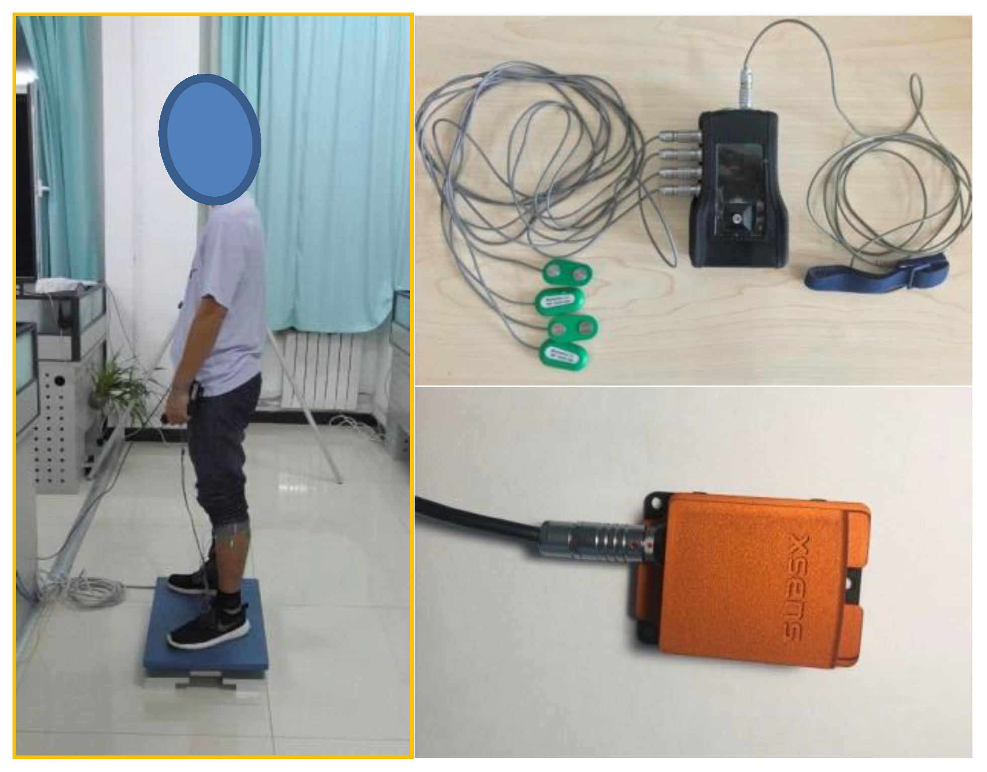
An inertial measurement unit (IMU) sensor (MTI-300-2A5G4, Xsens Technologies B.V., Enschede, NED) was attached to the shank to record the ankle joint kinematics data (i.e., joint angle, angular velocity and linear acceleration, with a sampling frequency of 300 Hz). A force plate (AMTI BP400600, Advanced Mechanical Technology, Inc., Denver, CO, USA) with a sampling frequency of 1000 Hz was used to record ground reaction forces (GRFs) and calculate COP positions. The NI-DAQmx was used to record the six-channel analog outputs of the force plate. As the pushing trigger signal was also recorded by NI-DAQmx, the pushing time and force plate data were recoded synchronously. sEMG data were recorded from three muscles, namely, tibialis anterior (TA), gastrocnemius (GAS) and soleus (SOL) with a commercial apparatus (DataLog MWX8, Biometrics, Ladysmith, VA, USA). TA sEMG signals were recorded as references. The sEMG electrode attachment procedure followed the instructions from SENIAM. The sampling frequency of the sEMG was 1000 Hz, with differential amplification (gain: 1000) and common mode rejection (104 dB). Maximum voluntary contraction (MVC) tests were performed before the experiment, and used for sEMG signal normalization. Custom software was developed with VS 2010 (Visual Studio 2010, Microsoft Corporation, Redmond, WA, USA) to the fulfill data collection operations. A laptop was sufficient to run the software in real-time. The experimental setup is shown in Figure 4.
Analysis of variance (ANOVA) was performed to test the difference in VAF among different time points. T-test was used to examine differences in reflex gains among subjects and VAF of reflex model prediction results with and without acceleration gains.
2.5. Data Synchronization
In this paper, three apparatuses were used, and 10 channels of data were recorded. Because some of these apparatuses provided no hardware synchronization interface, a two-step data synchronization method was developed.
In the first step, the recording command was sent to the apparatuses simultaneously by the host computer. There was a 5 s waiting period to ensure that all of the apparatuses had started up. The data received by the host computer were labeled with global timestamps. There were still inevitable time delays resulting from hardware differences in command receipt and data sending among the different apparatuses. This kind of time delay could be tens of milliseconds, which influences the results and the corresponding explanation. Therefore, in the second step, a cross-correlation (CC) method was implemented to further modify the timestamps.
The CC function can be described as:
where Rxy is the CC coefficient and tlag represents the time shift between x and y. Rxy is at its maximum when x(t) and y(t + tlag) are maximally related. The tlag at that maximum point is the time delay. Timestamps are modified by the corresponding tlag.
As forces are the instantaneous results of interaction and are measured by analogous circuit, we assume that there is no time delay in force data. Consequently, torque data calculated from force plate recordings were used as common signals. Ankle kinematic and kinetics data timestamps were adjusted by the tlag of linear acceleration and torque data. Because no external assisting force was applied in the experiment, leg linear acceleration changes were caused instantaneously by the change in ankle joint torque. Muscle activation data timestamps (the same with the sEMG timestamps) were adjusted by the tlag of muscle activation and torque data. According to the results of the currently existing research [32], in order to represent the electromechanical delays, the time from the onset of EMG activity and ankle joint torque variations, a 20 ms time lag is manually added to torque, angular acceleration, angular velocity and angle data.
3. Experimental Results
3.1. Push-Recovery Movement
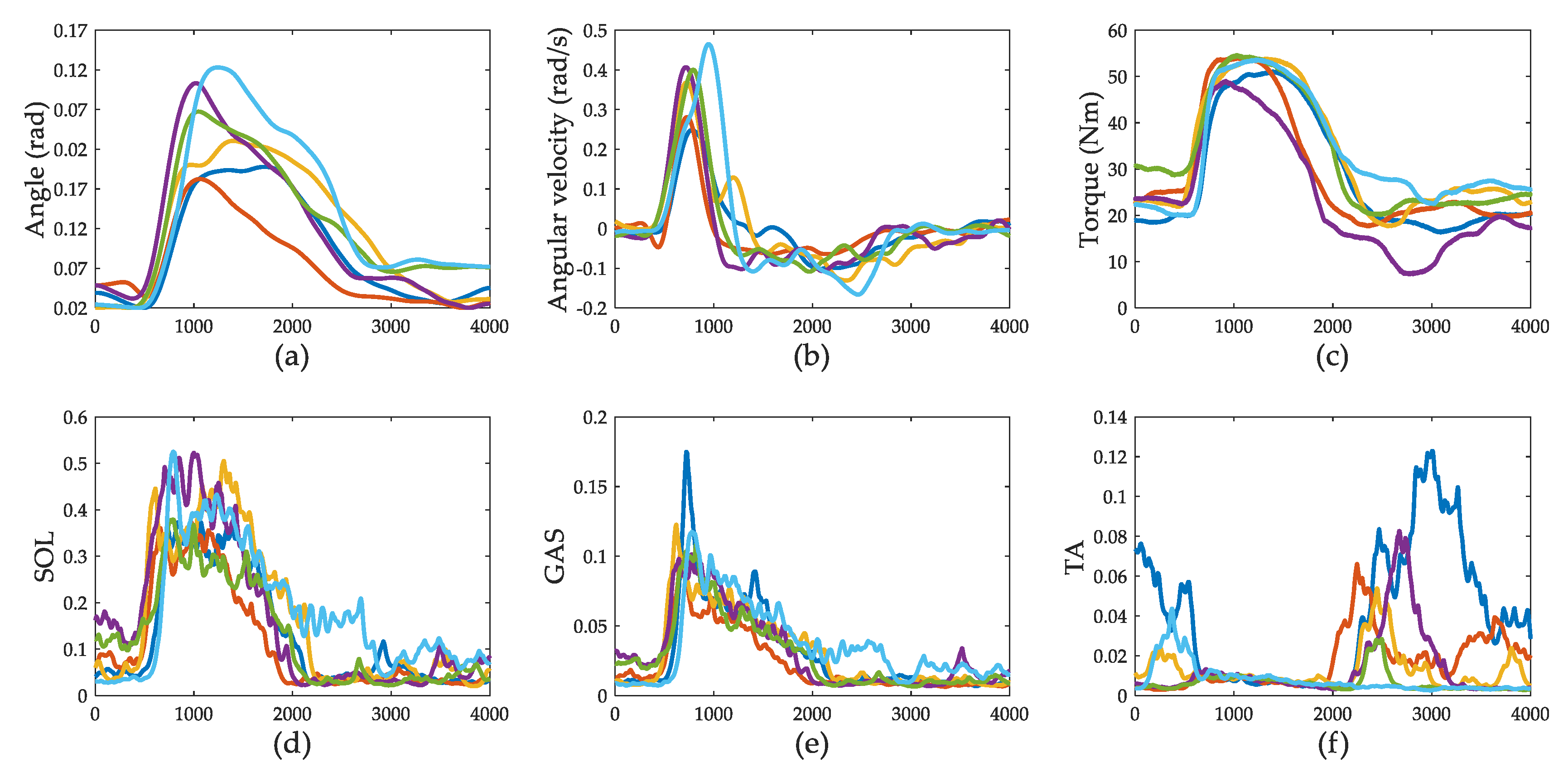
The experimental results for subject A are shown in Figure 5. The interval is 4 s, starting from 500 ms before perturbation. As soon as the disturbance is exerted on the back of the subject, the ankle joint angular velocity increases quickly in the negative direction, and the body of the subject leans forward. Ankle joint torque increases slightly. About 100–150 ms later, ankle joint torque increases sharply and stops the increasing trend of angular velocity. About 500 ms after the disturbance is exerted, the ankle joint torque reaches its maximum. There is a plateau-like part lasting for about 1 s after the ankle joint torque reaches its maximum. Ankle joint torque changes slowly in this part and behaves like a parabolic trajectory. Then, ankle joint torque decreases to the quiet standing level, followed by a small circular peak-to-peak up-and-down change in amplitude. This period lasts for about 2 s. For each trial, the absolute peak backward velocity is about 2.7 times (2.7 ± 0.8) smaller than the leaning forward velocity. It takes about 500 ms to stop the leaning forward trend and takes another 2500 ms to pull the body back to the equilibrium posture.
3.2. Muscle Activation
SOL and GAS contract to generate positive ankle joint torque. The activation of SOL and GAS last for about 1.5 s. TA becomes inactive (around 0.005, as shown in Figure 5f) when SOL and GAS are activated. TA is re-activated when activations of SOL and GAS are below 2 to 3%. This phenomenon is the so-called reciprocal inhibition. The stretch of the extensor muscles inhibits the activity of flexor motor neurons, and vice versa. When TA is re-activated, the ankle joint angle is still located within the lean forward range (above 0.02 rad from 2 to 3 s). We assume that the behavior of this part is controlled by the high-level nervous system interference.
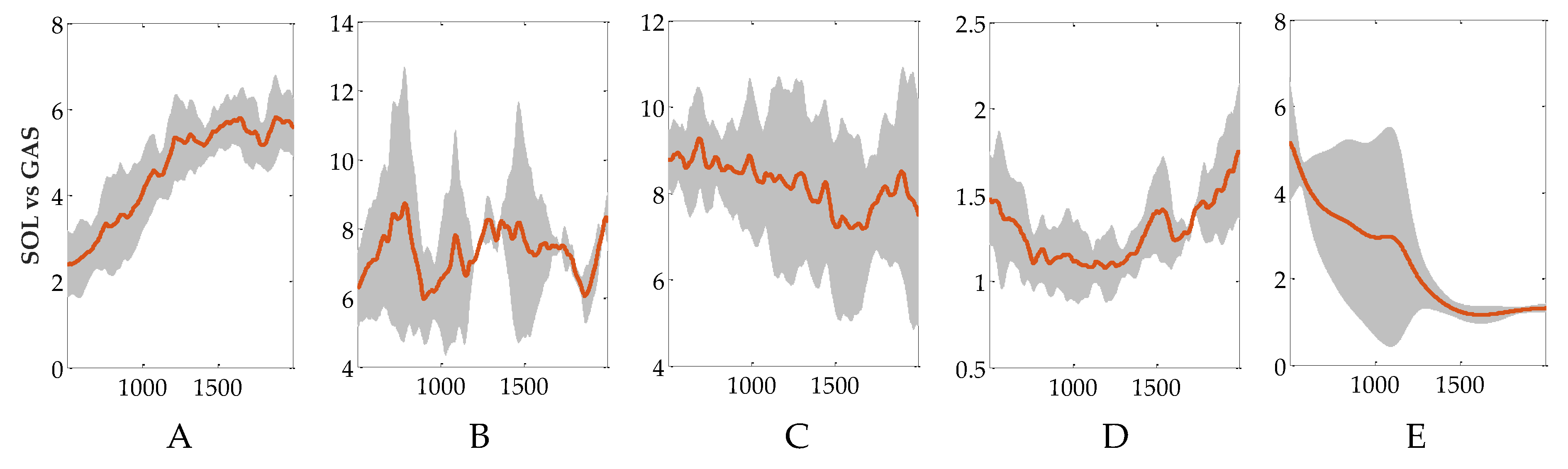
This alternate-active phenomenon appears in all five subjects. We separate the push-recovery process into two parts: the calf control part, in which SOL and GAS are active, and the TA control part, in which TA is active. The activation ratios between SOL and GAS of the five subjects in calf control part are shown in Figure 6. For subject A, the ratio increases. For subjects B and C, the ratio varies around a constant level. For subject D, the ratio is like a ‘valley’. For subject E, the ratio decreases. Given that SOL is the uniarticular muscle and GAS is the biarticular muscle, it seems that different movement manners are adopted among subjects. However, the ratios are greater than 1, which means that the muscle activation level of SOL is larger than that of GAS. The maximum muscle force of SOL is larger than GAS. SOL contributes more to torque production during this period. The purpose of the calf control part seems to be to stop the leaning forward trend in the trunk quickly and to produce a gross pull-back torque. As the body leans forward, the calf muscles are likely to be stretched. The reflex control model described in Equation (3) is applied in this part to predict the calf muscle activations.
In the TA control parts, the activation level of TA varies from 2 to 10%. The calf muscles and TA are co-contracted. Co-contraction of antagonistic muscles can increase joint stiffness while keeping the same torque level [43]. Thus, joint stability increases. It is helpful to increase joint stiffness to prevent CoM moving to the “joint-heel” side. As the supporting area of the human foot from the ankle joint to the heel is smaller than that from the ankle joint to the toe, there is less room left in the “joint-heel” part to adjust CoP (or ankle joint torque) to counteract gravity while maintaining ankle strategy. No significant ankle joint angle overshoot (below 0.02 rad) can be observed in the experiment (as shown in Figure 5a). The purpose of the TA control part seems to be to smoothly adjust body movement to stop at an upright posture, preventing too much overshoot in the opposite direction.
3.3. Evaluation of Reflex Control Model
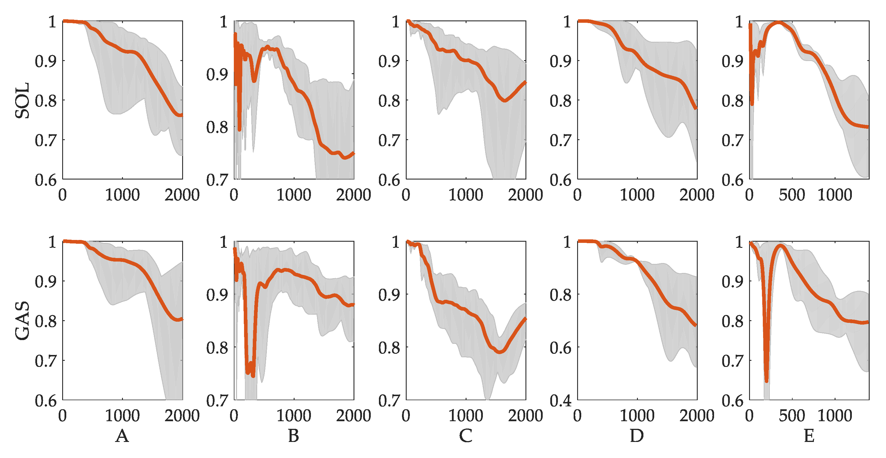
The VAF values of all five subjects vary with the change of time-increasing point, as displayed in Figure 7. The overall tendency can be broken into three parts. In the first part (from before 450 to 1000 ms), the values of VAF are above 90%. At the end of this part, values of VAF decrease. In the second part (from 500 ms to 1200 ms), the VAF values are within the range from 70% to 90%. In the third part (after 1200 ms), the values of VAF decrease continuously as the time increases.
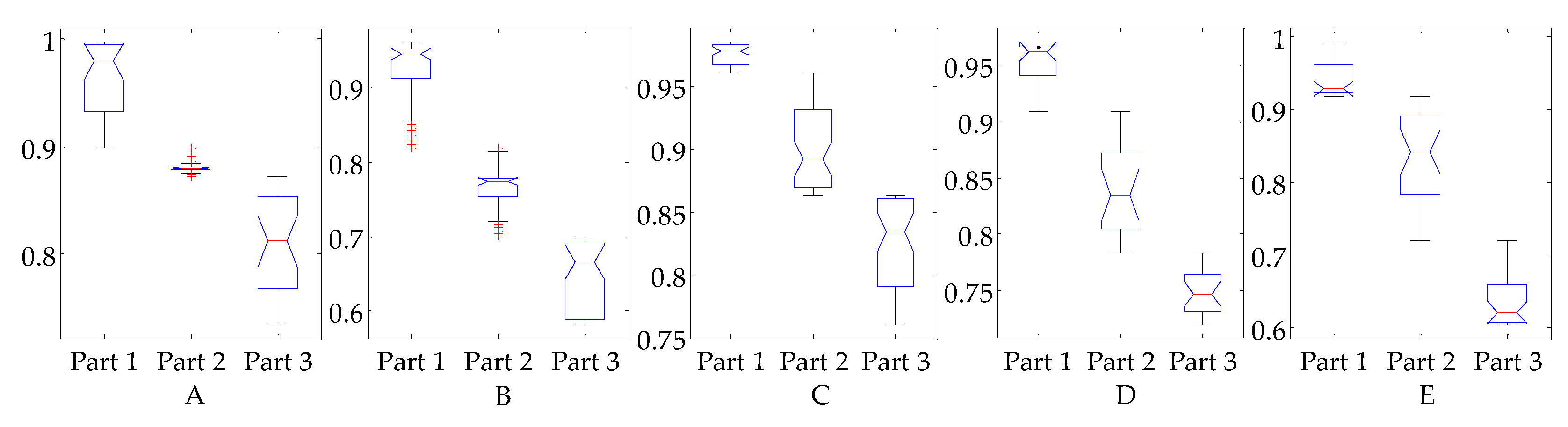
A one-way ANOVA test was performed on the three parts. The VAF values were collected from the six trials. As time points were different among trials, the following rule was used: the first part is collected from 200 ms before the time point at which angular velocity changes the direction; the second part is collected from 200 ms after the angular velocity direction change; the third part is collected from 200 ms before the end. Each part collects 20 points of VAF values for each trial. The results are depicted in Figure 8. For all five subjects, since p values are smaller than 0.01, it can be inferred that the aforementioned three parts are significantly different. Given the root mean square error (RMSE) between prediction and measured activations, the changing trend between the three parts shows that the reflex model fits the change in the first 450 to 1000 ms of calf muscle activation level well (RMSE around 0.03), as well as obtaining a fair result over a longer time period (RMSE from 0.03 to 0.08) and an unpromising result for the overall period (RMSE above 0.10). These experimental results may indicate that reflex dominates the first 400 to 1000 ms, while more complicated control mechanisms may be involved as time increases.
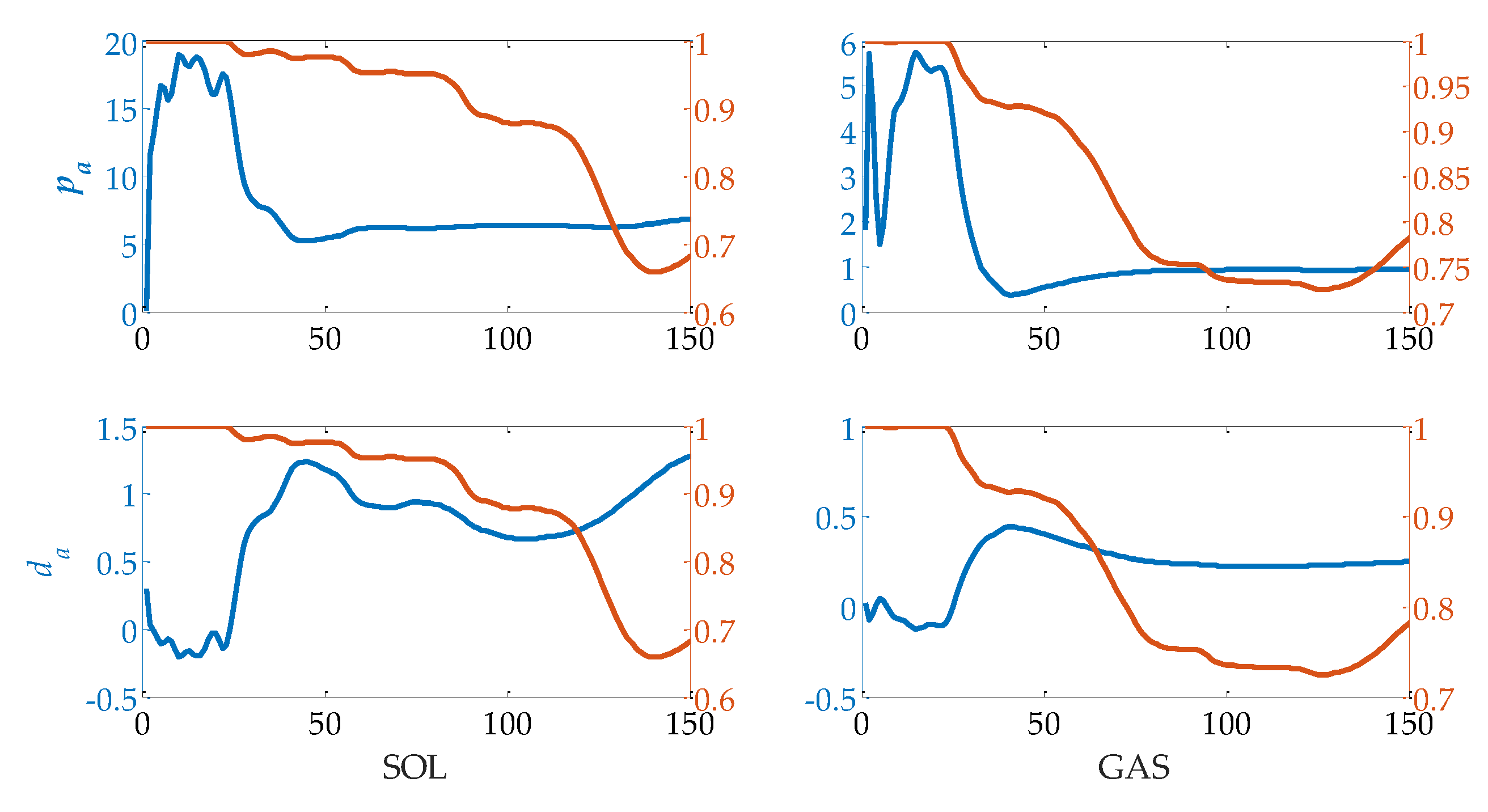
The variations of pa and da of subject A in one trial are shown in Figure 9. At the early stage of this trial, values of pa and da change rapidly at first, and subsequently remain stable when a sufficient amount of recorded data is applied. On the other hand, VAF decreases with the increase of time or the amount of recorded data (as shown in Figure 6). There is a tradeoff between VAF and stable reflex parameters. The time point at which VAF is above 90% and the reflex parameters are within a stable range is selected. In this paper, the period from the beginning of muscle activation to the selected time point is called the forepart of muscle activation. For four of the subjects, the time point is close to the time point at which the direction of joint angular velocity changes. For the left one, it is about 200–300 ms ahead of direction change. If we assume that calf muscle fiber length changes with the variation of ankle joint angle, this result will be consistent with the mechanism of stretch reflex. Muscle spindle senses the stretch motion of muscle fibers. When ankle joint angular velocity changing its direction or muscle fibers starting contraction, the spindle is not under a stretch condition, and the stretch reflex model is no longer suitable.
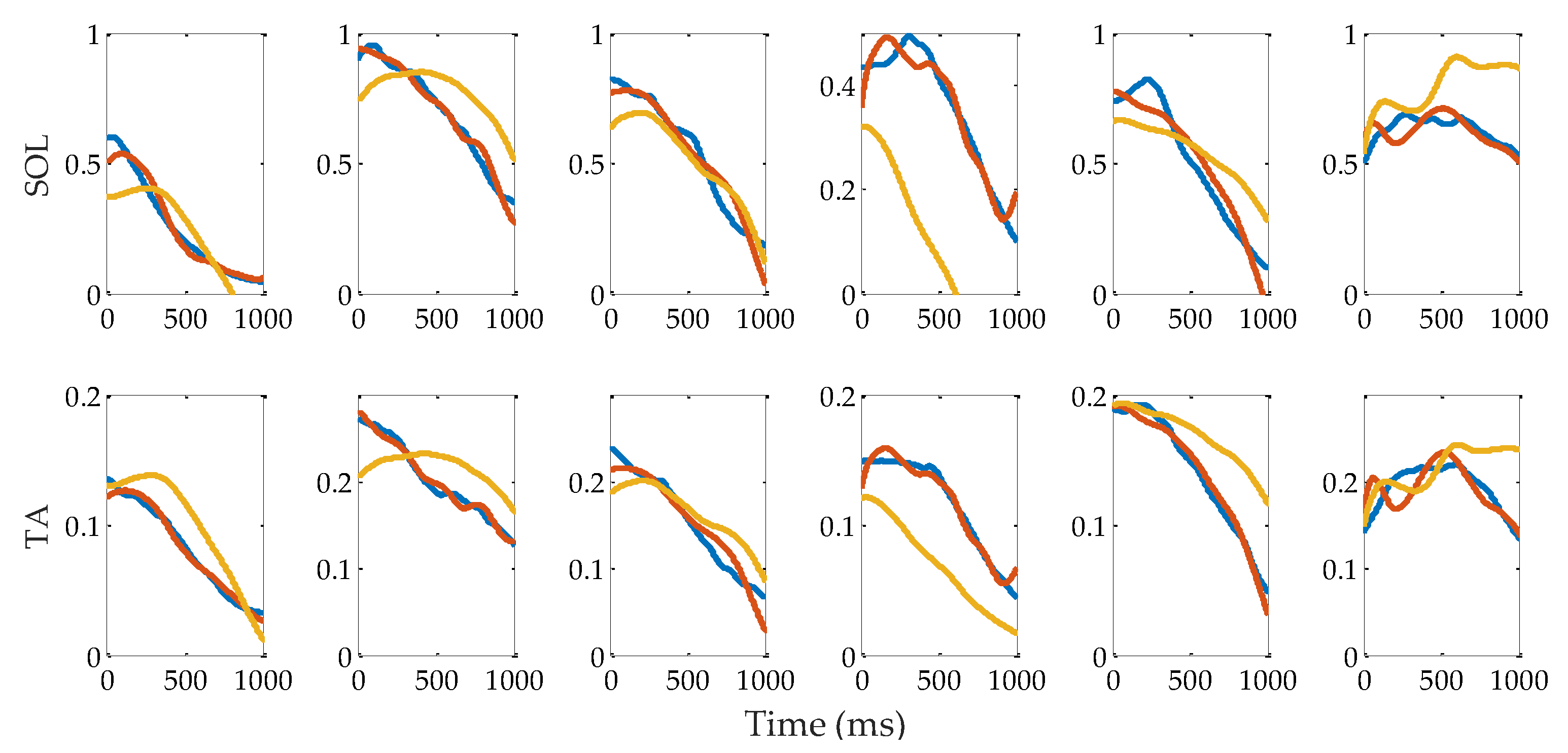
The reflex control model fitting results of forepart of subject A are shown in Figure 10, where the blue, red and yellow lines, respectively, are the recorded muscle activations, the prediction results with gains calculated from each trial, and the prediction results using the mean values of the gains. The VAF values of SOL and GAS between the red lines and the blue lines are 94.8 ± 1.3% and 95.7 ± 1.8%, respectively. Between the yellow lines and the blue lines, they are 88.2 ± 6.1% and 90.4 ± 7.5%, respectively. The RMSEs of SOL and GAS between the red lines and the blue lines are 0.03 ± 0.02 and 0.007 ± 0.004, respectively. Between the yellow and blue lines, they are 0.09 ± 0.03 and 0.024 ± 0.008, respectively. The p values for the one-way ANOVA test of the VAFs between the red lines and the yellow lines are 0.033 for SOL and 0.082 for GAS. In terms of the RMSEs, the p values are 0.019 and 0.0035 for SOL and GAS, respectively. Considering a significance level of 0.01, there are no significant differences between the red lines and yellow lines, except for the RMSEs of GAS.
The corresponding pa and da values of Figure 10 are listed in Table 1. The relative standard deviation (SD/Mean) of pa (SOL: 0.09, GAS: 0.19) is smaller than that of da (SOL: 0.69, GAS: 0.82). Compared with da, the values of pa do not change much. It seems that the da value is more sensitive to the disturbance.
Table 2 shows the mean reflex gains and prediction results for the remaining four subjects. It can be easily observed from Table 2 that, in comparison to the individual calculation results, the values of VAF based on mean gains prediction decreases. The minimum decrease value is 2.0%, in the prediction of the GAS activation of subject B, while the maximum value is 6.6%, in the prediction of the SOL activation of subject A. However, it is important to note that, despite showing a decreasing tendency in the values of VAF, they are still at a relatively high level (above 85%), which shows the potential of the mean value in real-time implementation. Differences in reflex gains among the subjects are listed in Table 3 (repeated two-sample t-test, 0.05 significance level). From this table, one can see that, on the one hand, the difference of pa among subjects B, C and D is not significant, while on the other hand, the difference of da among subjects A, C and D is also not significant.
Equation (1) is implemented to evaluate the rest of the muscle activation level. That is to say, the starting point is the end time point of the forepart, and the ending point is the time point at which muscle activation level returns to its quiet level. The fitting results for subject A are shown in Figure 11, in which the lines with different colors have the same meanings as those shown in Figure 10. The VAF values of SOL and GAS between the red lines and the blue lines are 90.4 ± 8.1% and 93.0 ± 7.5%, respectively. Between the yellow lines and the blue lines, they are, respectively, 64.9 ± 12.9% and 67.5 ± 20.9%. RMSEs of SOL and GAS between the red lines and the blue lines are 0.05 ± 0.02 and 0.01 ± 0.005, respectively. Between the yellow and the blue lines, they are 0.17 ± 0.09 and 0.041 ± 0.020, respectively. The p values of the one-way ANOVA test of the VAFs between the red lines and the yellow lines are 0.0021 for SOL and 0.009 for GAS. For RMSE, they are 0.0035 and 0.0017, respectively. Compared with the forepart, the fitting results with individual gains and mean gains are significantly different at a significance level of 0.01 with respect to VAF and RMSE. Mean pa and da values of the rest part for the five subjects are listed in Table 4. Mean pa values for the rest part significantly differ from those of the forepart for subject A, B, D and E at a significance level of 0.05 with respect to SOL. With the exception of Subject D, the other four subjects likely adopt different da values to control SOL. Mean pa values of GAS are different for subjects B and D, and mean da values of GAS are different for subjects A and C (significance level 0.05). Compared to the results of fitting muscle activation from the forepart start point, VAF values increased (p < 0.01) when only fitting the rest part. Fitting results by mean gains are significantly decreased compared with individual gains, apart from subjects C (SOL) and E.
The results noted above show the feasibility of the model described by Equation (1) for the rest of the muscle activation level with different gains. Mean gains are not acceptable for fitting the muscle activation of the rest part for most of the subjects.
3.4. Ankle Joint Torque Prediction Results
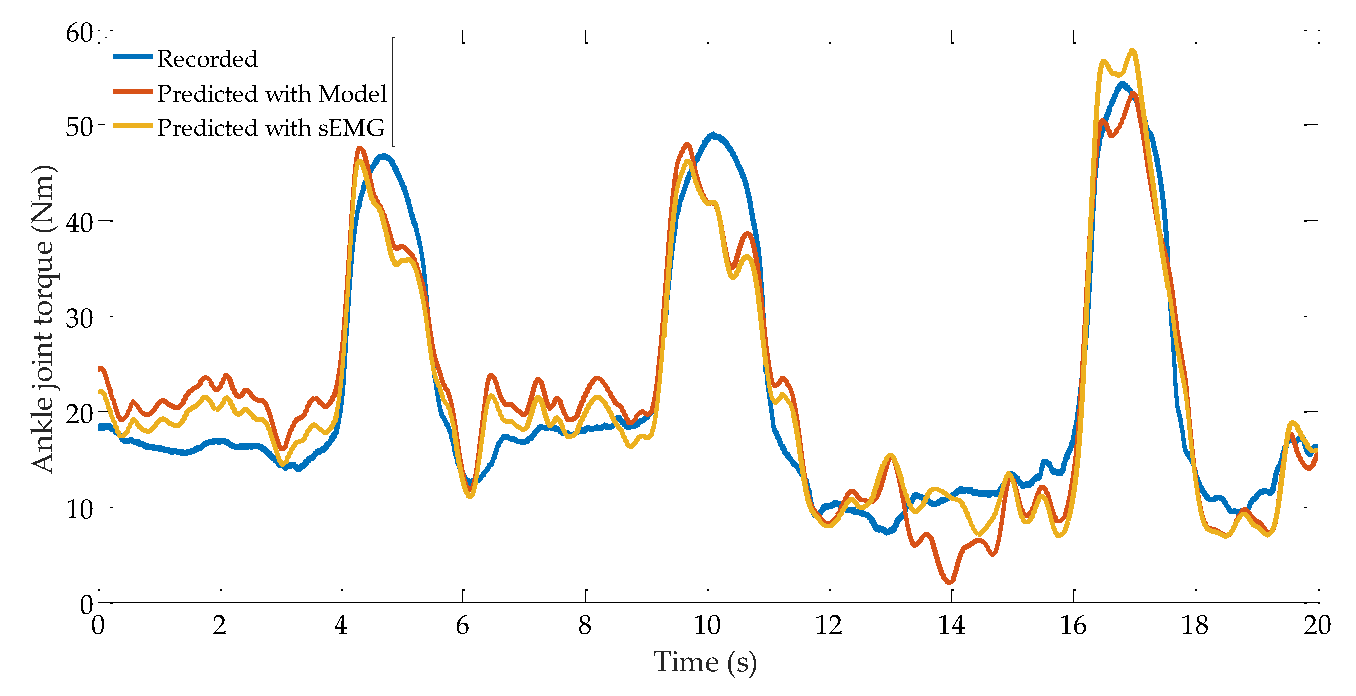
The muscular model-based ankle torque prediction results are shown in Figure 12. In this figure, the prediction results and the torque recorded by the force plate are distinguished by red and blue lines, respectively. According to the data comprising this figure, it can be seen that the values of RMSE and VAF are, respectively, 4.9 Nm and 0.86. The calibrated parameters for the different muscles of subject B are given in Table 5. It is noticeable from this table that, although there is no guarantee that each parameter is correct with the proposed optimal method, the multiplication of these parameters is relatively accurate.
The correlation coefficient between muscle activations and ankle joint torque is greater than 0.95. This implies that muscle activations and torque are highly linear with each other. Also, this can be further demonstrated by noting that fl and fv in Equation (8) are almost constant (LCE << LCE0, VCE << VCE0). Thus, Equation (8) can be simplified as follows:
where i represents different muscles. ci can be obtained by regression algorithm.
In Figure 12, the prediction result is depicted as an orange line. Based on the data comprising the prediction result in this figure, it can be seen that the values of RMSE and VAF for the prediction results are 4.0 Nm and 0.88, respectively. These results indicate that a relatively high accuracy ankle joint torque can be obtained under the condition of ‘ankle strategy’ push-recovery movement by using the muscle activation level.
4. Discussion
The high VAF values and low RMSE of the fitting results indicate that muscle reflex control may greatly dominate the forepart of upright standing push-recovery. The same formula is still workable for fitting the rest muscle activation part of the motion with different gains. The two-piecewise behavior revealed by the experimental results shows that different gains should be implemented in order to fulfill upright standing push-recovery motion. As a non-invasive way of exploring the internal neural control mechanism involved in push-recovery movement, the proposed method is feasible for calculating calf muscle reflex gains.
4.1. Comparison with Currently Existing Studies
Muscle stretch reflex is often expressed in a PD-like form. It is rational to use proportional and derivative components to predict muscle activation levels, as muscle spindle is sensitive to change in muscle fiber length and rate of change. The reflex model used in this paper is similar to that described in [32], in which the muscle activation was predicted by PD algorithm during quiet standing. Since the inputs of the model shown in [32] are the position and velocity of CoM, this model reflects the reaction of CNS to the body’s global state. Nevertheless, there is still a strong necessity to reveal the joint-level local response to the disturbance or the external environment, especially in the case of controlling a joint-level exoskeleton device and prostheses. The experimental results of this paper evaluate the possibility of using local ankle joint kinematics information to predict calf muscle activation. Local reflex control can release the burden from a higher-level controller, such as the human brain or a robot central controller. Moreover, the situation in [32] can be regarded as quasi-static, whereas the situation in this paper is dynamic. Our results imply that the stretch reflex control model is suitable, at least in the forepart of upright standing push-recovery movement.
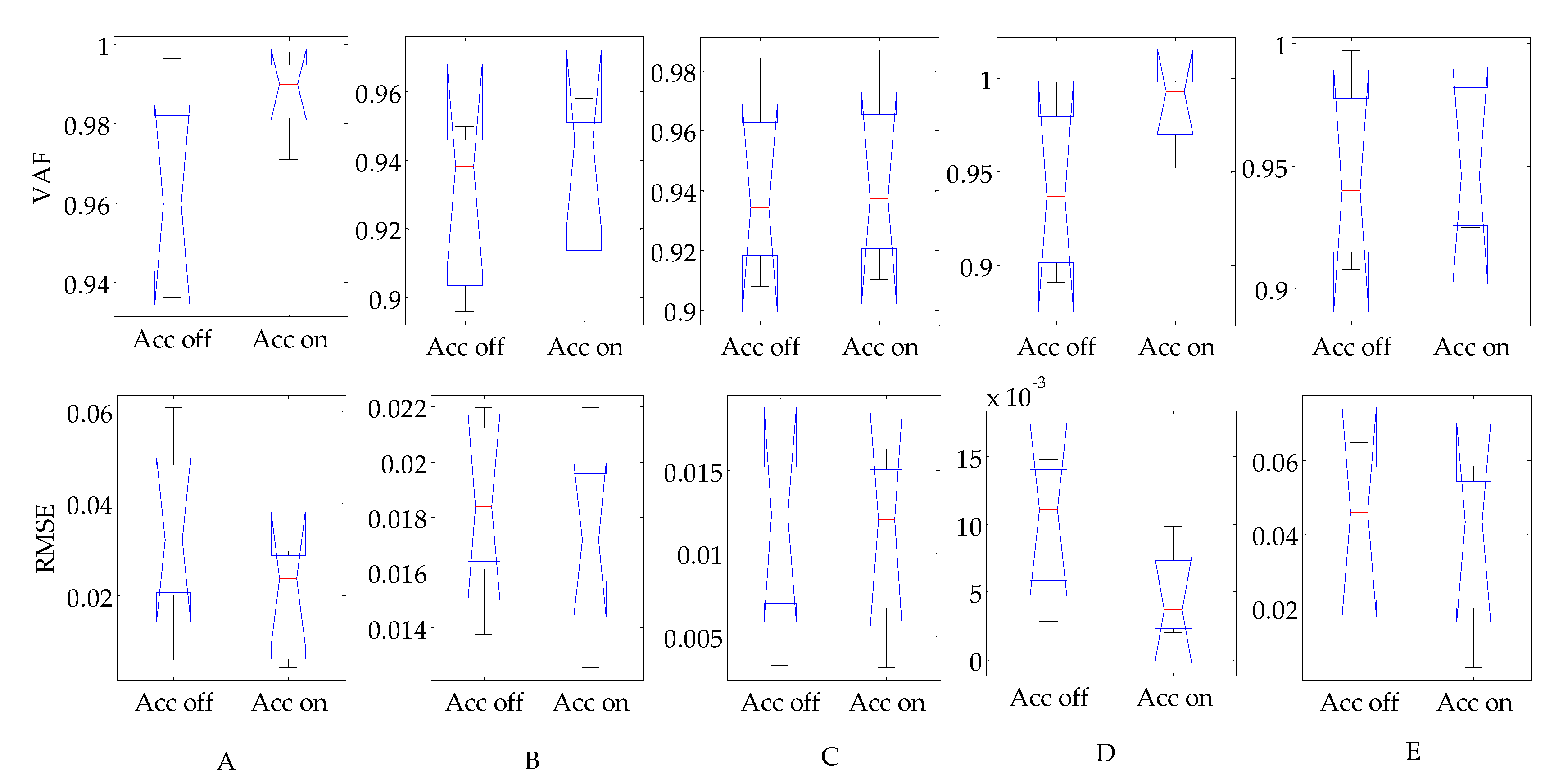
As acceleration has been suggested to be an important part of muscle activation prediction [27], this study validates the effect of adding an acceleration item into Equation (1) with the same data used in Section 3.3 for the prediction result. To this end, a one-way ANOVA is performed in this study. The results are shown in Figure 13. For all five subjects, the differences between the prediction results in the cases including the acceleration item and those without are insignificant (at a significance level of 0.01). This indicates that the acceleration item may not dominate the forepart of ankle joint torque control under our experimental conditions. The feedback delay between the ankle joint and the vestibular system may be the longest, as the ankle joint is the most distal joint to the vestibular system. This long delay will cause disadvantages in local ankle joint control. Moreover, the experimental study conducted in [27] is based on a cat, whose height differs greatly from that of humans, which may result in acceleration having greater affects than those found in our study.
4.2. The Role of Ankle Joint Reflex Control
Based on the results shown in Section 3.4, the muscle activation and the ankle joint torque are relatively linear with each other. Calf muscles work in an isometric-like manner. Substituting Equation (2) into Equation (13), a linearized muscle reflex force controller can be yielded as follows:
where cpa and cda are in Nm/rad and Nm/rad/s, and have equal units of stiffness and damping, respectively. Based on the model denoted by Equation (14), it can be concluded that muscle reflex seems to try to control the MTUs of the ankle joint to achieve a spring-damper-like behavior. A limited disturbance will eventually vanish in such a system.
There are two components in the concept of ankle joint impedance, that is, intrinsic and reflex components [44]. The intrinsic component arises from the musculoskeletal system tissues’ mechanical properties and the muscle fiber’s tonic contraction. The reflex component originates from muscle activation due to sensory responses to stretch. As reported in [45], the reflex component accounts for 10% of the required impedance to remaining upright in a quiet standing posture (compared with mgh). However, our experimental results show that the reflex component accounts for more than 10% of the required impedance to complete the push-recovery motion, which indicates that the reflex component plays a more important role in maintaining balance in a dynamic situation than in a static situation.
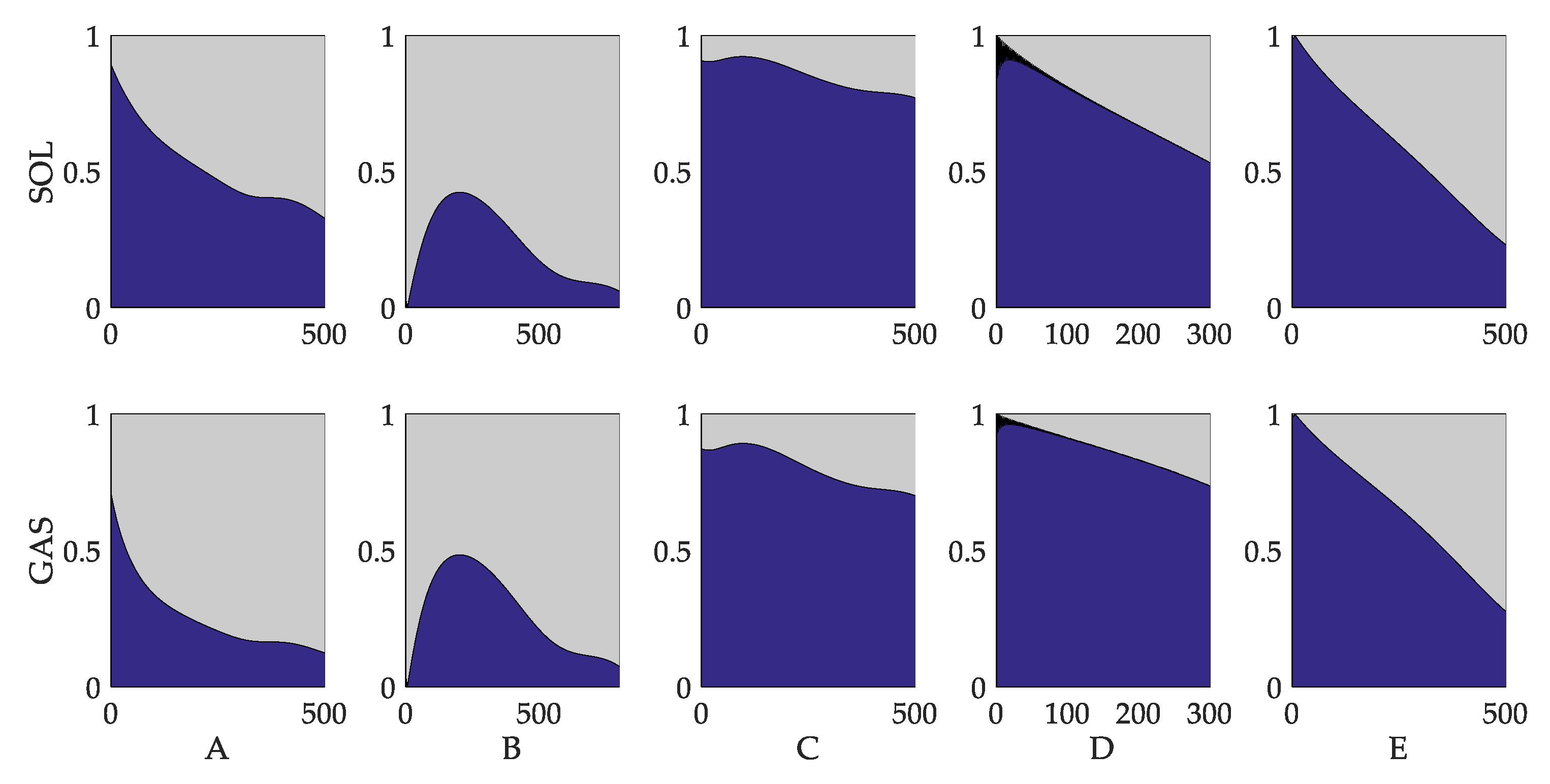
The contribution of the damper component, namely, the component evoked by velocity, is significant. The ratio between fiber length and velocity contributions is depicted in Figure 14. The velocity component accounts for more than 60% in the first 300 to 500 ms in subjects C, D and E. For the other two subjects, the velocity parts account for 20 to 80% in the first 500 ms. According to [9], angular velocity is assumed to be a factor that effects reflex gains under the circumstances of upright standing ankle strategy. In the early phase of push-recovery, the velocity part leads to increasingly rapid muscle activation and assists in inhibiting the trend of leaning forward. According to the results obtained in this study, the damper component is of great significance in the forepart of push-recovery.
4.3. Implementation of the Proposed Method
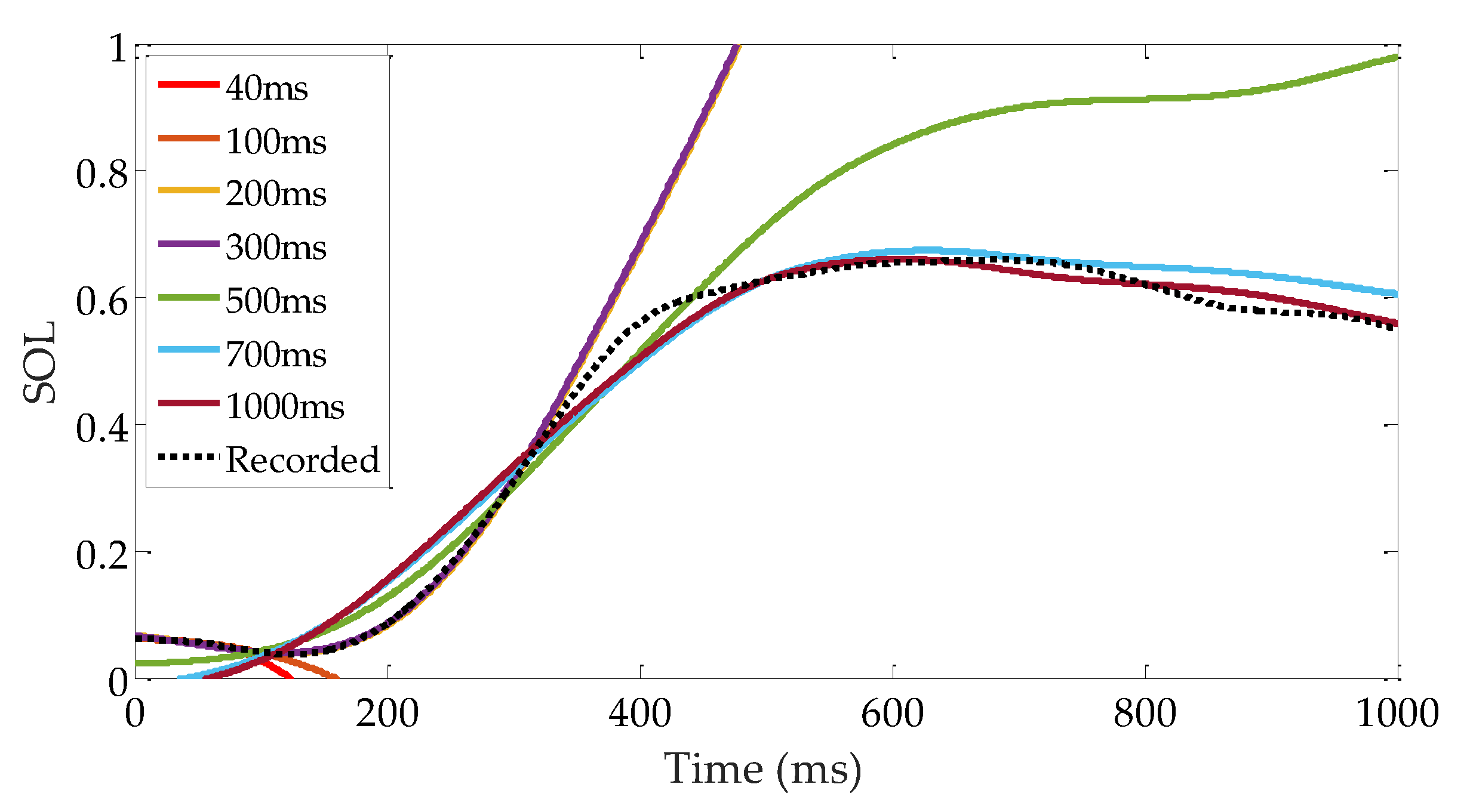
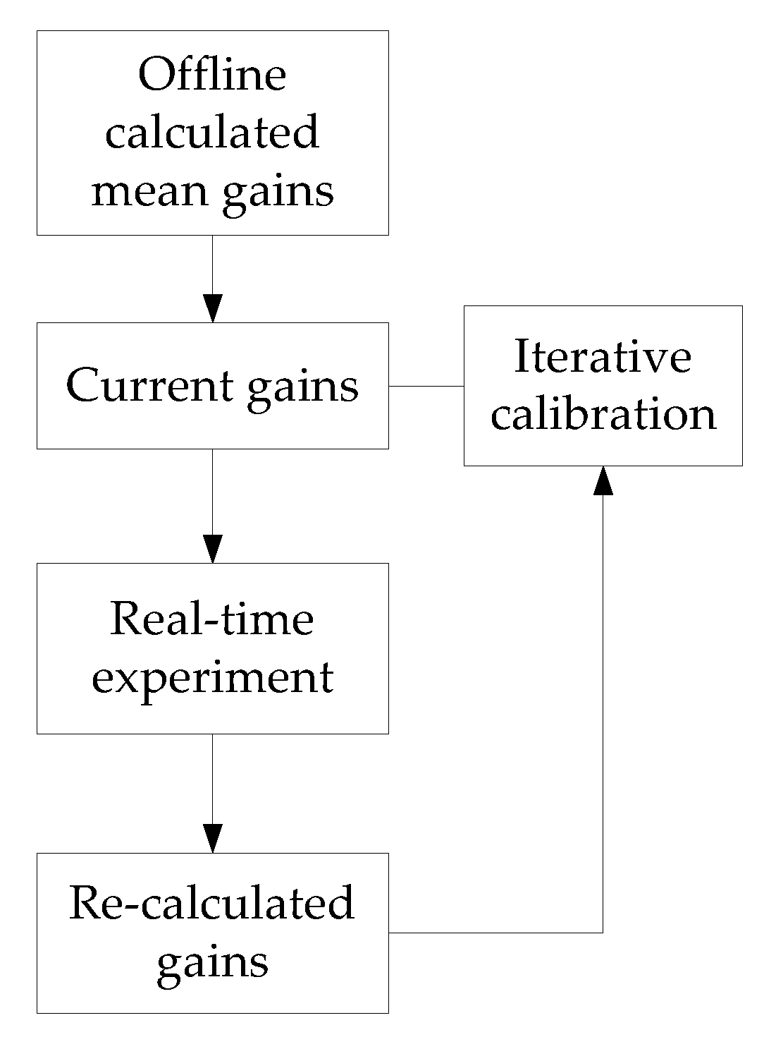
It is desirable to calculate the reflex gain in real time (maybe in 1-10 ms). As sEMG and kinematic signals are very sensitive to noise, the gains calculated from short-range data are useless. Figure 15 shows the prediction results with gains calculated from different lengths of data. The gains calculated using a data set 400–700 ms long are feasible for representing the reflex. However, a 400 ms time interval is too long for controlling a robotic device. Fortunately, the gains are within a limited range. An average value is beneficial to fitting muscle activation with a 1–2% decrease in VAF, which provides a feasible iterative approach to problems in controlling robotic device. The reflex gains can be calculated beforehand and used as initial control gains. As demonstrated in Figure 16, by comparing the current reflex gains and the initial gains, a modification can be applied based on a step-by-step manner using some intelligent methods.
4.4. Selection of sEMG Low-Pass Cutoff Frequency
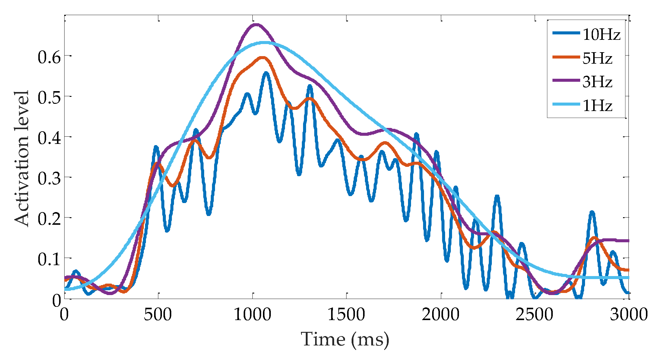
The low-pass cutoff frequency is one factor that affects the sEMG processing results. The low-pass filter is used to acquire a smooth muscle activation envelope [39]. It has been demonstrated that applying a low-pass filter is highly convenient in the study of muscle force and limb motion prediction, as the muscle behaves like a low-pass filter [46]. Thus far, even though the low-pass filter has been extensively investigated, no standard results have been reported to act as guidelines for how to set or obtain appropriate values. Values from 1 to 10 Hz in 1 Hz increments are tested in this study. Figure 17 shows the comparison among the different cutoff frequencies for subject A. As the cutoff frequency drops, the evelope becomes smoother. Clear fluctuations can be found by using a 10 Hz cutoff frequency. Almost no fluctuation could be observed below 3 Hz. The envelope turns into a smooth line with a cutoff frequency of 1 Hz.
It is convenient to obtain a smooth value in engineering applications. However, too much information loss also has profound influences on the results. Table 6 summarizes the reflex gains and VAF values of muscle activation prediction under different cutoff frequencies. From this table, one can observe that pa and VAF values increase, whereas da value first increases (until 3 Hz) and then decreases in the case where the cutoff frequency decreases. We assume that the fluctuation influences the reflex gain calculation and model prediction results seriously in the 10 Hz case. In this case, the reflex gains are inaccurate, and the VAF value is low. With the smoothing of fluctuation, its influence on the reflex gains and VAF decreases. This improvement for da stops when the cutoff frequency is lower than 3 Hz. In the 1 Hz case, the da value decreases to about 40% compared with the 3 Hz case, and in some cases, the value becomes negative, which means that the physiological meaning has been lost. The increase of pa value may be explained by the amplitude (or the muscle activation level) increasing with the decreasing of the cutoff frequency (except the 1 Hz case). The maximum muscle activation amplitude and the pa values increase by 24% (0.55 in 10 Hz and 0.68 in 3 Hz) and 30%, respectively. pa value remains almost unchanged when cutoff frequency is lower than 3 Hz. This result indicates that the da component dominates the 3–5 Hz range and the pa component dominates the lower frequencies.
5. Conclusions
Reflex control is evaluated on calf muscles during upright standing push-recovery using the ankle joint strategy in this paper. A time-increasing search method, in which the reflex gains can be obtained through a simple regression algorithm, is proposed to test the feasibility of the reflex model for fitting real muscle activations. The experimental results show that the reflex model is able to well fit the forepart and rest part of calf muscle activation with different gains. Under the reflex control mechanism, the ankle joint forms a spring-damping-like system to resist external disturbance. This simple and effective control mechanism causes the ankle joint dynamic properties to become suitable for environmental interaction. This study also investigates the human internal control mechanism underlying the push-recovery movement. The two-piecewise results indicate that controlling ankle joint robotic devices with constant gains may be insufficient to assist the human upright standing push-recovery motion. The obtained results will be applied in the control of an exoskeleton device to assist human upright standing balance in the near future.
Author Contributions
M.P. provided the conceptualization, methodology and original draft preparation of this manuscript; X.X. wrote the software together with B.T. and took charge of data curation; B.T. support the development of the software and revised the manuscript in English together with M.P. and Z.J. K.X. provided the conceptualization together with M.P.; Z.J. provided funding support and reviewed the manuscript.
Funding
This research was funded by National Natural Science Foundation of China, grant number 61603284 and 51575412.
Acknowledgments
The authors thanks for the kind help of the five volunteers.
Conflicts of Interest
The authors declare no conflict of interest. The founding sponsors had no role in the design of the study; in the collection, analyses, or interpretation of data; in the writing of the manuscript, and in the decision to publish the results.
References
- Yang, C.; Ganesh, G.; Haddadin, S.; Parusel, S.; Albu-Schaeffer, A.; Burdet, E. Human-like adaptation of force and impedance in stable and unstable interactions. IEEE Trans. Robot. 2011, 27, 918–930. [Google Scholar] [CrossRef]
- Collins, S.H.; Wiggin, M.B.; Sawicki, G.S. Reducing the energy cost of human walking using an unpowered exoskeleton. Nature 2015, 522, 212–215. [Google Scholar] [CrossRef] [PubMed] [Green Version]
- Mooney, L.M.; Herr, H.M. Biomechanical walking mechanisms underlying the metabolic reduction caused by an autonomous exoskeleton. J. Neuroeng. Rehabil. 2016, 13, 1–12. [Google Scholar] [CrossRef] [PubMed]
- Rajasekaran, V.; Aranda, J.; Casals, A.; Pons, J.L. An adaptive control strategy for postural stability using a wearable robot. Robot. Auton. Syst. 2015, 73, 16–23. [Google Scholar] [CrossRef] [Green Version]
- Hogen, N. Impedance control: An approach to manipulation. J. Dyn. Syst.-Trans. ASME 1985, 107, 17. [Google Scholar] [CrossRef]
- Sentis, L.; Khatib, O. A whole-body control framework for humanoids operating in human environments. In Proceedings of the 2006 IEEE International Conference on Robotics and Automation, Orlando, FL, USA, 15–18 May 2006; pp. 2641–2648. [Google Scholar] [CrossRef]
- McMahon, T.A. Muscles, Reflexes, and Locomotion; Princeton University Press: Princeton, NJ, USA, 1984; pp. 139–161. ISBN 0-691-08322-3. [Google Scholar]
- Fitzpatrick, R.C.; Gorman, R.B.; Burke, D.; Gandevia, S.C. Postural proprioceptive reflexes in standing human subjects: Bandwidth of response and transmission characteristics. J. Physiol. 1992, 458, 69–83. [Google Scholar] [CrossRef]
- Masani, K.; Popovic, M.R.; Nakazawa, K.; Kouzaki, M.; Nozaki, D. Importance of body sway velocity information in controlling ankle extensor activities during quiet stance. J. Neurophysiol. 2003, 90, 3774–3782. [Google Scholar] [CrossRef]
- Finley, J.M.; Dhaher, Y.Y.; Perreault, E.J. Contributions of feed-forward and feedback strategies at the human ankle during control of unstable loads. Exp. Brain Res. 2012, 217, 53–66. [Google Scholar] [CrossRef] [PubMed]
- Peterka, R.J. Sensorimotor integration in human postural control. J. Neurophysiol. 2002, 88, 1097–1118. [Google Scholar] [CrossRef]
- Insperger, T.; Milton, J.; Stépán, G. Acceleration feedback improves balancing against reflex delay. J. R. Soc. Interface. 2013, 10, 20120763. [Google Scholar] [CrossRef] [PubMed]
- Prochazka, A.; Gillard, D.; Bennett, D.J. Positive force feedback control of muscles. J. Neurophysiol. 1997, 77, 3226–3236. [Google Scholar] [CrossRef] [PubMed]
- Prochazka, A.; Gillard, D.; Bennett, D.J. Implications of positive feedback in the control of movement. J. Neurophysiol. 1997, 77, 3237–3251. [Google Scholar] [CrossRef] [PubMed]
- Pfeifer, S.; Vallery, H.; Hardegger, M.; Riener, R.; Perreault, E.J. Model-based estimation of knee stiffness. IEEE Trans. Bio-Med. Eng. 2012, 59, 2604–2612. [Google Scholar] [CrossRef] [PubMed]
- Misgeld, B.J.; Zhang, T.; Lüken, M.J.; Leonhardt, S. Model-based estimation of ankle joint stiffness. Sensors 2017, 17, 713. [Google Scholar] [CrossRef] [PubMed]
- Clancy, E.A.; Liu, L.; Liu, P.; Moyer, D.V.Z. Identification of constant-posture EMG-torque relationship about the elbow using nonlinear dynamic models. IEEE Trans. Bio-Med. Eng. 2012, 59, 205–212. [Google Scholar] [CrossRef] [PubMed]
- Yang, C.; Zeng, C.; Liang, P.; Li, Z.; Li, R.; Su, C.Y. Interface design of a physical human–robot interaction system for human impedance adaptive skill transfer. IEEE Trans. Autom. Sci. Eng. 2018, 15, 329–340. [Google Scholar] [CrossRef]
- Ajoudani, A.; Tsagarakis, N.; Bicchi, A. Tele-impedance: Teleoperation with impedance regulation using a body–machine interface. Int. J. Robot. Res. 2012, 31, 1642–1656. [Google Scholar] [CrossRef]
- Ju, Z.; Liu, H. Human hand motion analysis with multisensory information. IEEE-ASME Trans. Mech. 2014, 19, 456–466. [Google Scholar] [CrossRef]
- Lee, H.; Krebs, H.I.; Hogan, N. Multivariable dynamic ankle mechanical impedance with active muscles. IEEE Trans. Neural Syst. Rehabil. Eng. 2014, 22, 971–981. [Google Scholar] [CrossRef]
- Hashemi, J.; Morin, E.; Mousavi, P.; Hashtrudi-Zaad, K. Surface EMG force modeling with joint angle based calibration. J. Electromyogr. Kinesiol. 2013, 23, 416–424. [Google Scholar] [CrossRef]
- Artemiadis, P.K.; Kyriakopoulos, K.J. A switching regime model for the EMG-based control of a robot arm. IEEE Trans. Syst. Man Cybern. B 2001, 41, 53–63. [Google Scholar] [CrossRef]
- Hill, A.V. The heat of shortening and the dynamic constants of muscle. Proc. R. Soc. Lond. Ser. B-Biol. Sci. 1938, 126, 136–195. [Google Scholar] [CrossRef] [Green Version]
- Zajac, F.E. Muscle and tendon: Properties, models, scaling, and application to biomechanics and motor control. Crit. Rev. Biomed. Eng. 1989, 17, 359–411. [Google Scholar]
- Durandau, G.; Farina, D.; Sartori, M. Robust real-time musculoskeletal modeling driven by electromyograms. IEEE Trans. Bio-Med. Eng. 2018, 65, 556–564. [Google Scholar] [CrossRef]
- Lockhart, D.B.; Ting, L.H. Optimal sensorimotor transformations for balance. Nat. Neurosci. 2007, 10, 1329–1336. [Google Scholar] [CrossRef]
- Geyer, H.; Herr, H. A muscle-reflex model that encodes principles of legged mechanics produces human walking dynamics and muscle activities. IEEE Trans. Neural Syst. Rehabil. Eng. 2010, 18, 263–273. [Google Scholar] [CrossRef]
- Nitish, T.; Geyer, H. Toward balance recovery with leg prostheses using neuromuscular model control. IEEE Trans. Bio-Med. Eng. 2016, 63, 904–913. [Google Scholar] [CrossRef]
- Batts, Z.; Song, S.; Geyer, H. Toward a virtual neuromuscular control for robust walking in bipedal robots. In Proceedings of the IEEE/RSJ International Conference on Intelligent Robots and Systems, Hamburg, Germany, 28 September–2 October 2015; pp. 6318–6323. [Google Scholar]
- Winter, D.A.; Patla, A.E.; Prince, F.; Ishac, M.; Gielo-Perczak, K. Stiffness control of balance in quiet standing. J. Neurophysiol. 1998, 80, 1211–1221. [Google Scholar] [CrossRef]
- Vette, A.H.; Masani, K.; Nakazawa, K.; Popovic, M.R. Neural-mechanical feedback control scheme generates physiological ankle torque fluctuation during quiet stance. IEEE Trans. Neural Syst. Rehabil. Eng. 2010, 18, 86–95. [Google Scholar] [CrossRef]
- Emmens, A.R.; van Asseldonk, E.H.; van der Kooij, H. Effects of a powered ankle-foot orthosis on perturbed standing balance. J. Neuroeng. Rehabil. 2018, 15, 50–62. [Google Scholar] [CrossRef]
- Cafolla, D.; Marco, C. Design and simulation of humanoid spine. New Trends Mech. Mach. Sci. 2015, 24, 585–593. [Google Scholar] [CrossRef]
- Cafolla, D.; Chen, I.M.; Ceccarelli, M. An experimental characterization of human torso motion. Front. Mech. Eng. 2015, 10, 311–325. [Google Scholar] [CrossRef]
- Fitzpatrick, R.; Burke, D.; Gandevia, S.C. Loop gain of reflexes controlling human standing measured with the use of postural and vestibular disturbances. J. Neurophysiol. 1996, 76, 3994–4008. [Google Scholar] [CrossRef] [PubMed]
- Blum, K.P.; D’Incamps, B.L.; Zytnicki, D.; Ting, L.H. Force encoding in muscle spindles during stretch of passive muscle. PLoS Comput. Biol. 2017, 13, e1005767. [Google Scholar] [CrossRef]
- Maganaris, C.N. Force-length characteristics of the in vivo human gastrocnemius muscle. Clin. Anat. 2003, 16, 215–223. [Google Scholar] [CrossRef]
- Buchanan, T.S.; Lloyd, D.G.; Manal, K.; Besier, T.F. Estimation of muscle forces and joint moments using a forward-inverse dynamics model. Med. Sci. Sports Exerc. 2005, 37, 1911–1916. [Google Scholar] [CrossRef]
- OpenSim Documentation—Musculoskeletal Models. Available online: https://simtk-confluence.stanford.edu/display/OpenSim/Musculoskeletal+Models#MusculoskeletalModels-OpenSimCoreModels (accessed on 10 May 2018).
- Roberts, T.J. The integrated function of muscles and tendons during locomotion. Comp. Biochem. Phys. A 2002, 133, 1087–1099. [Google Scholar] [CrossRef]
- Hansen, N. The CMA evolution strategy: A tutorial. arXiv 2016, arXiv:1604.00772. [Google Scholar]
- Hogan, N. Adaptive control of mechanical impedance by coactivation of antagonist muscles. IEEE Trans. Autom. Control 1984, 29, 681–690. [Google Scholar] [CrossRef]
- Kearney, R.E.; Stein, R.B.; Parameswaran, L. Identification of intrinsic and reflex contributions to human ankle stiffness dynamics. IEEE Trans. Bio-Med. Eng. 1997, 44, 493–504. [Google Scholar] [CrossRef]
- Vlutters, M.; Boonstra, T.A.; Schouten, A.C.; van der Kooij, H. Direct measurement of the intrinsic ankle stiffness during standing. J. Biomech. 2015, 48, 1258–1263. [Google Scholar] [CrossRef] [PubMed]
- Potvin, J.R.; Brown, S.H.M. Less is more: High pass filtering, to remove up to 99% of the surface EMG signal power, improves EMG-based biceps brachii muscle force estimates. J. Electromyogr. Kinesiol. 2004, 14, 389–399. [Google Scholar] [CrossRef] [PubMed]
Figure 1.
Schematic of upright standing push-recovery. m is the mass of the body (excluding the foot part); θ is the ankle joint angle; the clockwise direction is defined as positive; CoP is the point of center of pressure; GRFz is the z-axis ground reaction force; Fm is the calf muscle force.
Figure 1.
Schematic of upright standing push-recovery. m is the mass of the body (excluding the foot part); θ is the ankle joint angle; the clockwise direction is defined as positive; CoP is the point of center of pressure; GRFz is the z-axis ground reaction force; Fm is the calf muscle force.

Figure 2.
Ankle joint neural-muscular control model. Muscle fiber parameters LCE and VCE are converted from θ and via ‘Ankle anatomy structure’.
Figure 2.
Ankle joint neural-muscular control model. Muscle fiber parameters LCE and VCE are converted from θ and via ‘Ankle anatomy structure’.

Figure 3.
Schematic diagram of the proposed time-increasing searching method. The reflex model is applied to fit the muscle activation step by step to find a proper reflex-domain time interval.
Figure 3.
Schematic diagram of the proposed time-increasing searching method. The reflex model is applied to fit the muscle activation step by step to find a proper reflex-domain time interval.

Figure 4.
Upright standing push-recovery. Left picture shows a subject standing on the force plate. Pushing force is exerted on his back. Right upper picture shows the sEMG device. Right lower picture shows the IMU sensor.
Figure 4.
Upright standing push-recovery. Left picture shows a subject standing on the force plate. Pushing force is exerted on his back. Right upper picture shows the sEMG device. Right lower picture shows the IMU sensor.

Figure 5.
Experimental results for subject A. Each color represents one trial. There are six trials. The x-axis is the time in ms. (a) shows the measurement of ankle joint angle. (b) represents the ankle joint angular velocity. (c) shows the ankle joint torque. (d) shows the muscle activation level of SOL. (e) shows the muscle activation level of GAS. (f) shows the muscle activation level of TA.

Figure 6.
Activation ratio of SOL to GAS in calf control part. Red line is the mean value. Gray area is the standard deviation (SD). Subgraph (A) to (E) represents the results of subject A to E, respectively.
Figure 6.
Activation ratio of SOL to GAS in calf control part. Red line is the mean value. Gray area is the standard deviation (SD). Subgraph (A) to (E) represents the results of subject A to E, respectively.

Figure 7.
VAF values of reflex prediction results. Each column represents one subject. The red lines are the mean values of six trials. The gray areas represent maximum and minimum values.
Figure 7.
VAF values of reflex prediction results. Each column represents one subject. The red lines are the mean values of six trials. The gray areas represent maximum and minimum values.

Figure 8.
Boxplot of the three parts from five subjects. All the p values (ANOVA) are much smaller than 0.01.
Figure 8.
Boxplot of the three parts from five subjects. All the p values (ANOVA) are much smaller than 0.01.

Figure 9.
Variations of pa and da of a single trial. The blue lines are the pa and da values. The red lines are the VAF values of prediction results.
Figure 9.
Variations of pa and da of a single trial. The blue lines are the pa and da values. The red lines are the VAF values of prediction results.

Figure 10.
Reflex model fitting results of the forepart of subject A of the six trials. The blue lines are the muscle activation calculated from the measured sEMG signals. The red lines are the prediction results using individually calibrated reflex gains. The yellow lines are the prediction results using mean reflex gains.

Figure 11.
Reflex model prediction results for the rest part of subject A over the six trials. The blue lines are the muscle activation calculated from the measured sEMG signals. The red lines are the prediction results using individually calibrated reflex gains. The yellow lines are the prediction results using mean reflex gains.

Figure 12.
Ankle joint torque prediction results with musculoskeletal model and sEMG.

Figure 13.
Boxplot of prediction results with and without acceleration. Column (A) to (E) represents the results of subject A to E, respectively. The p values of the first row are 0.041, 0.601, 0.922, 0.153 and 0.790, respectively. The p values of the second row are 0.164, 0.638, 0.958, 0.160 and 0.872, respectively.

Figure 14.
Ratio of da part contribution to pa part contribution. Column (a) to (e) represents the results of subject A to E, respectively. The blue area the contribution of the da part. The gray area represents the contribution of the pa part. Each column represents one subject. The x-axis is the time.

Figure 15.
Muscle activation prediction results using different reflex gains. The gains are calculated from different lengths of data. The dotted line is the measured muscle activation. The results show that the prediction results are not acceptable if the length of the data is too short.
Figure 15.
Muscle activation prediction results using different reflex gains. The gains are calculated from different lengths of data. The dotted line is the measured muscle activation. The results show that the prediction results are not acceptable if the length of the data is too short.

Figure 16.
Diagram of implementation of the proposed method. The mean values of reflex gains are used as initial gains for a robotic device controller. An iterative calibration is applied to modified the reflex gains.
Figure 16.
Diagram of implementation of the proposed method. The mean values of reflex gains are used as initial gains for a robotic device controller. An iterative calibration is applied to modified the reflex gains.

Figure 17.
Muscle activations calculated with different low-pass cutoff frequencies. Results with 10, 5, 3 and 1 Hz are plotted to make the graph easy to read.
Figure 17.
Muscle activations calculated with different low-pass cutoff frequencies. Results with 10, 5, 3 and 1 Hz are plotted to make the graph easy to read.


Table 1.
SOL and GAS reflex gains of subject A of six trials.
| 1 | 2 | 3 | 4 | 5 | 6 | |
|---|---|---|---|---|---|---|
| pa of SOL | 6.20 | 6.12 | 5.34 | 6.90 | 6.85 | 6.82 |
| da of SOL | 0.91 | 0.50 | 1.02 | 0.19 | 0.24 | 0.29 |
| VAF 1 of SOL | 0.94/0.96 | 0.92/0.93 | 0.78/0.95 | 0.91/0.95 | 0.83/0.95 | 0.88/0.92 |
| RMSE 2 of SOL | 0.03/0.02 | 0.11/0.06 | 0.13/0.04 | 0.08/0.01 | 0.10/0.05 | 0.09/0.05 |
| pa of GAS | 0.84 | 1.06 | 0.85 | 1.31 | 1.08 | 1.31 |
| da of GAS | 0.28 | 0.03 | 0.14 | 0.05 | 0.11 | 0.07 |
| VAF of GAS | 0.77/0.94 | 0.94/0.96 | 0.88/0.93 | 0.97/0.97 | 0.96/0.97 | 0.90/0.95 |
| RMSE of GAS | 0.02/0.005 | 0.04/0.01 | 0.03/0.01 | 0.01/0.002 | 0.02/0.01 | 0.02/0.01 |
1 The value of VAF is listed as (VAF of mean gains prediction)/(VAF of individual calculated gains prediction). 2 The value of RMSE is listed in the same way as VAF.
Table 2.
The forepart mean reflex gains for all five subjects.
| A | B | C | D | E | |
|---|---|---|---|---|---|
| pa of SOL | 6.37 ± 0.61 | 2.43 ± 0.37 | 3.59 ± 0.81 | 2.44 ± 0.51 | 14.51 ± 3.70 |
| da of SOL | 0.52 ± 0.36 | 1.92 ± 0.52 | 0.28 ± 0.14 | 0.36 ± 0.28 | 0.81 ± 0.63 |
| VAF 1 | 88.2/94.8 | 89.0/91.6 | 88.2/90.4 | 89.4/94.2 | 90.4/92.2 |
| pa of GAS | 1.08 ± 0.21 | 1.90 ± 0.70 | 4.06 ± 1.01 | 4.65 ± 1.30 | 8.36 ± 2.78 |
| da of GAS | 0.11 ± 0.09 | 0.20 ± 0.08 | 0.31 ± 0.18 | 1.09 ± 0.49 | 0.66 ± 0.34 |
| VAF | 90.4/95.7 | 90.3/92.3 | 87.2/91.3 | 88.3/92.1 | 87.3/91.5 |
1 The value of VAF is listed as (VAF of mean gains prediction)/(VAF of individual calculated gains prediction).
Table 3.
t-test p values of gains among subjects.
| B | C | D | E | |
|---|---|---|---|---|
| A | 0.001, 0.002 1 | 0.018, 0.865 | 0.001, 0.561 | 0.038, 0.265 |
| B | 0.094, 0.002 | 0.955, 0.005 | 0.008, 0.131 | |
| C | 0.109, 0.630 | 0.014, 0.279 | ||
| D | 0.009, 0.368 |
1 The two p values are for pa and da, respectively.
Table 4.
The rest part mean reflex gains for all five subjects.
| A | B | C | D | E | |
|---|---|---|---|---|---|
| pa of SOL 1 | 16.84 ± 7.51(<0.01) | 8.88 ± 9.356(<0.01) | 3.75 ± 1.02(0.826) | 2.00 ± 1.07(0.03) | 9.61 ± 4.70(0.03) |
| pd of SOL | −1.13 ± 3.71(<0.01) | 0.70 ± 0.82(0.031) | 0.73 ± 0.60(0.017) | 0.56 ± 0.43(0.17) | 0.93 ± 1.06(0.03) |
| VAF | 64.9/90.4(<0.01) | 67.0/77.0(<0.01) | 77.6/88.1(0.185) | 59.3/83.2(<0.01) | 73.7/88.7(0.23) |
| pa of GAS | 2.97 ± 1.79(0.108) | 0.67 ± 0.52(0.021) | 6.46 ± 1.94(0.087) | 1.88 ± 1.05(<0.01) | 6.11 ± 2.50(0.397) |
| pd of GAS | −0.13 ± 0.98(<0.01) | 0.18 ± 0.09(0.428) | 0.33 ± 0.30(0.029) | 1.11 ± 1.40(0.43) | 0.35 ± 0.48(0.09) |
| VAF | 67.5/93.0(<0.01) | 76.9/82.7(0.027) | 90.0/95.3(0.045) | 60.1/80.1(<0.01) | 79.3/86.4(0.47) |
1 The value with the form of mean ± SD (p value, compared with forepart value).
Table 5.
Musculoskeletal model parameters of subject B.
| Muscle | FMAX (N) | θp (°) | LCE0 (cm) | VCE0 (cm/s) |
|---|---|---|---|---|
| SOL | 4572.3 | 28.3 | 4.78 | 50 |
| GAS | 2225.7 | 12 | 5.78 | 60 |
| TA 1 | 1148.9 | 9.6 | 6.04 | 60 |
1 The parameters of TA are listed here, because to obtain accurate ankle joint torque, the contribution of TA is needed.
Table 6.
Variation in reflex gains and reflex prediction VAF values of subject B with different low-pass cutoff frequencies.
Table 6.
Variation in reflex gains and reflex prediction VAF values of subject B with different low-pass cutoff frequencies.
| 10Hz | 7Hz | 6Hz | 5Hz | 4Hz | 3Hz | 2Hz | 1Hz | |
|---|---|---|---|---|---|---|---|---|
| pa | 4.06 | 4.35 | 4.48 | 4.66 | 4.93 | 5.35 | 5.84 | 5.33 |
| da | 0.38 | 0.42 | 0.44 | 0.46 | 0.48 | 0.48 | 0.39 | 0.19 |
| VAF | 0.74 | 0.84 | 0.86 | 0.88 | 0.91 | 0.95 | 0.98 | 0.98 |
© 2019 by the authors. Licensee MDPI, Basel, Switzerland. This article is an open access article distributed under the terms and conditions of the Creative Commons Attribution (CC BY) license (http://creativecommons.org/licenses/by/4.0/).
Share and Cite
MDPI and ACS Style
Pang, M.; Xu, X.; Tang, B.; Xiang, K.; Ju, Z. Evaluation of Calf Muscle Reflex Control in the ‘Ankle Strategy’ during Upright Standing Push-Recovery. Appl. Sci. 2019, 9, 2085. https://doi.org/10.3390/app9102085
AMA Style
Pang M, Xu X, Tang B, Xiang K, Ju Z. Evaluation of Calf Muscle Reflex Control in the ‘Ankle Strategy’ during Upright Standing Push-Recovery. Applied Sciences. 2019; 9(10):2085. https://doi.org/10.3390/app9102085
Chicago/Turabian StylePang, Muye, Xiangui Xu, Biwei Tang, Kui Xiang, and Zhaojie Ju. 2019. "Evaluation of Calf Muscle Reflex Control in the ‘Ankle Strategy’ during Upright Standing Push-Recovery" Applied Sciences 9, no. 10: 2085. https://doi.org/10.3390/app9102085
Note that from the first issue of 2016, this journal uses article numbers instead of page numbers. See further details here.