Prediction of Moment Redistribution in Statically Indeterminate Reinforced Concrete Structures Using Artificial Neural Network and Support Vector Regression

Abstract

In this paper, a new prediction model is proposed that fully considers the various parameters influencing the moment redistribution in statically indeterminate reinforced concrete (RC) structures by using the artificial neural network (ANN) and support vector regression (SVR). Twenty-four continuous RC beams and 12 continuous RC frames with various design parameters were tested to investigate the process of moment redistribution. Based on the experimental results obtained from this study and the published literature, a reliable database with 111 datasets was developed for the training and testing of the models. The predicted values of the proposed models, together with the estimations of the widely used code methods, were compared with the experimental results in the database. The analysis results showed that both the proposed ANN and SVR models exhibit high accuracy and reliability for the prediction of the moment redistribution.

1. Introduction

Statically indeterminate reinforced concrete (RC) structures are some of the most common structural forms in engineering design. Owing to the cracking of the concrete, the strain penetration of the reinforcement, and the formation and gradual rotation of the plastic hinge regions, the relative stiffness of each cross section changes constantly during the loading process, which causes a redistribution of internal forces in the statically indeterminate structure. In structural design, the moment redistribution is considered since it can help to avoid the reinforcement congestion at critical sections, thereby improving the convenience of the construction and the concreting conditions. Moreover, moment redistribution can help fully exploit the reserved capacity of the non-critical sections and achieve an economic design.

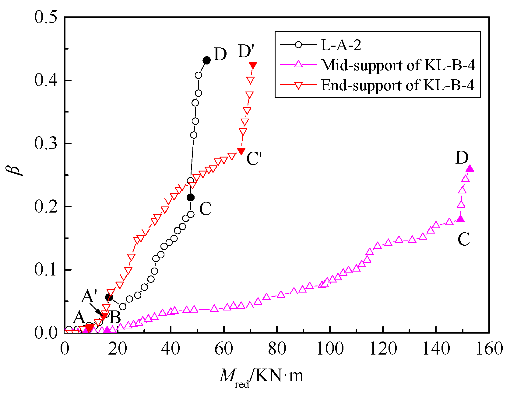
For practical applications, the current design codes allow designers to take advantage of linear elastic analysis with limit moment redistribution for structural design, in which the moment diagram derived from the elastic analysis of the structure is modified based on the degree of moment redistribution. Many definitions for measuring the moment redistribution have been proposed. The coefficient of the moment redistribution β, defined by Cohn [1] and adopted in various design codes, is shown in Equation (1):

$$\beta =\frac{M_{\mathrm{elast}}-M_{\mathrm{red}}}{M_{\mathrm{elast}}}$$

(1)

where M_elast is the elastic moment calculated by the elastic theory, M_red is the actual moment after moment redistribution, and β is between 0 and 1.

A reasonable consideration of the degree of the moment redistribution is important for the analysis and design of structures. Traditionally, moment redistribution is considered to be heavily dependent on the ductile behavior of the critical section [2]. In most design provisions, moment redistribution is mainly related to the neutral axis depth factor (the ratio of neutral axis depth to the section effective depth), since it can well characterize the ductility of a section by combining the characteristics of the materials and the geometry of the cross section. In fact, evaluation of the moment redistribution is complex because it depends on the rotation capacity of the plastic hinge as well as the variation in the stiffness distribution and the bond between the reinforcement and concrete [3]. Numerous studies have focused on the behavior and influencing factors of moment redistribution in statically indeterminate structures. Nearly all of these studies are based on a basic model of continuous beams subjected to static loads. By using the concept of ductility demand, the effects of various parameters, including slenderness, stiffness, ratio of tensile and compressive reinforcement, concrete strength, and strength of the reinforcement, on the moment redistribution in continuous RC beams were studied by Scholz [4] and Mostofinejad et al. [5]. Based on the experiments of continuous RC beams, Bagge et al. [3] concluded that a decrease in the tensile reinforcement and increase in the compression and transverse reinforcement would be beneficial for the moment redistribution. However, for high-strength concrete beams, the influence of the transverse reinforcement ratio is not significant, as observed in the experimental studies conducted by Carmo and Lopes [6]. Their study also indicated that the relationship between mid-span reinforcement ratio and intermediate-support reinforcement ratio had a significant effect on moment redistribution. Scott et al. [7] experimentally studied the whole process of the moment redistribution in continuous RC beams. Their results show that the moment redistribution evolves through several stages and the parameters, such as the cross-section size, concrete strength and arrangement of the reinforcement, affect the moment redistribution in each stage. In addition to the experimental studies, many theoretical methods have been proposed to investigate the effective behavior of continuous RC members. Oehlers et al. [8] developed a structural mechanics-based mathematical model for moment redistribution in continuous members, which was combined with the shear-friction approach [9], partial-interaction theory [10], and rigid body displacement. Through the application of this model, they concluded that moment redistribution increased with the decrease in the bond strength and the increase in the diameter of steel bars and concrete confinement. To study the entire nonlinear behavior of RC continuous beams, a finite element model based on the moment–curvature relationship and the Timoshenko beam theory was established by Lou et al. [11]. By using this model, the effect of many factors, such as the concrete strength, the relationship between the tensile reinforcement ratios at critical negative and positive moment regions, the relative stiffness, and the concrete confinement on moment redistribution were studied comprehensively.

As mentioned above, the mechanics of moment redistribution are incredibly complicated. The aim of this study was to propose a new model for accurate prediction of the moment redistribution that considers the various influential parameters as comprehensively as possible, while being convenient for the applications of practical engineering. In recent years, artificial intelligence techniques of artificial neural networks (ANNs) and support vector machines (SVMs) have exhibited great potential for solving various problems in civil engineering. Different from most methods used in civil engineering, ANN and SVM algorithms do not rely on the existing theories about structural mechanism, but employ high precision fitting to match the results to the real values as closely as possible [12]. These two models have been successfully applied to several areas in structural engineering, such as structural analysis [13,14,15], prediction of the shear resistance in beams [16,17,18,19] and compressive strength of columns [20,21,22,23], displacement determination of RC buildings [24], and estimation of the compressive strength for various types of concrete [25,26,27,28,29]. More recently, they were used to understand the behavior of structures under extreme conditions. Based on a back-propagation ANN, Ince [30] developed a fracture model to predict the fracture parameters of cementitious materials. Compared with the common non-linear fracture mechanics approaches, the ANN model was more reliable. In a separate study, Erdem [31] established an ANN model for determining the ultimate moment capacity of RC slabs in fire. The prediction values were compared with the results provided by the ultimate moment capacity equation, which showed the ANN model had a high degree of accuracy. To ensure the realistic fire performance of steel structures, Naser [32] used ANN to derive temperature-dependent thermal and mechanical material models for structural steel. The applicability of the models was validated using numerical case studies with a highly nonlinear finite element model. The results indicated that the proposed ANN models can significantly enhance the current state of structural fire design by developing a uniform representation of material properties at elevated temperatures.

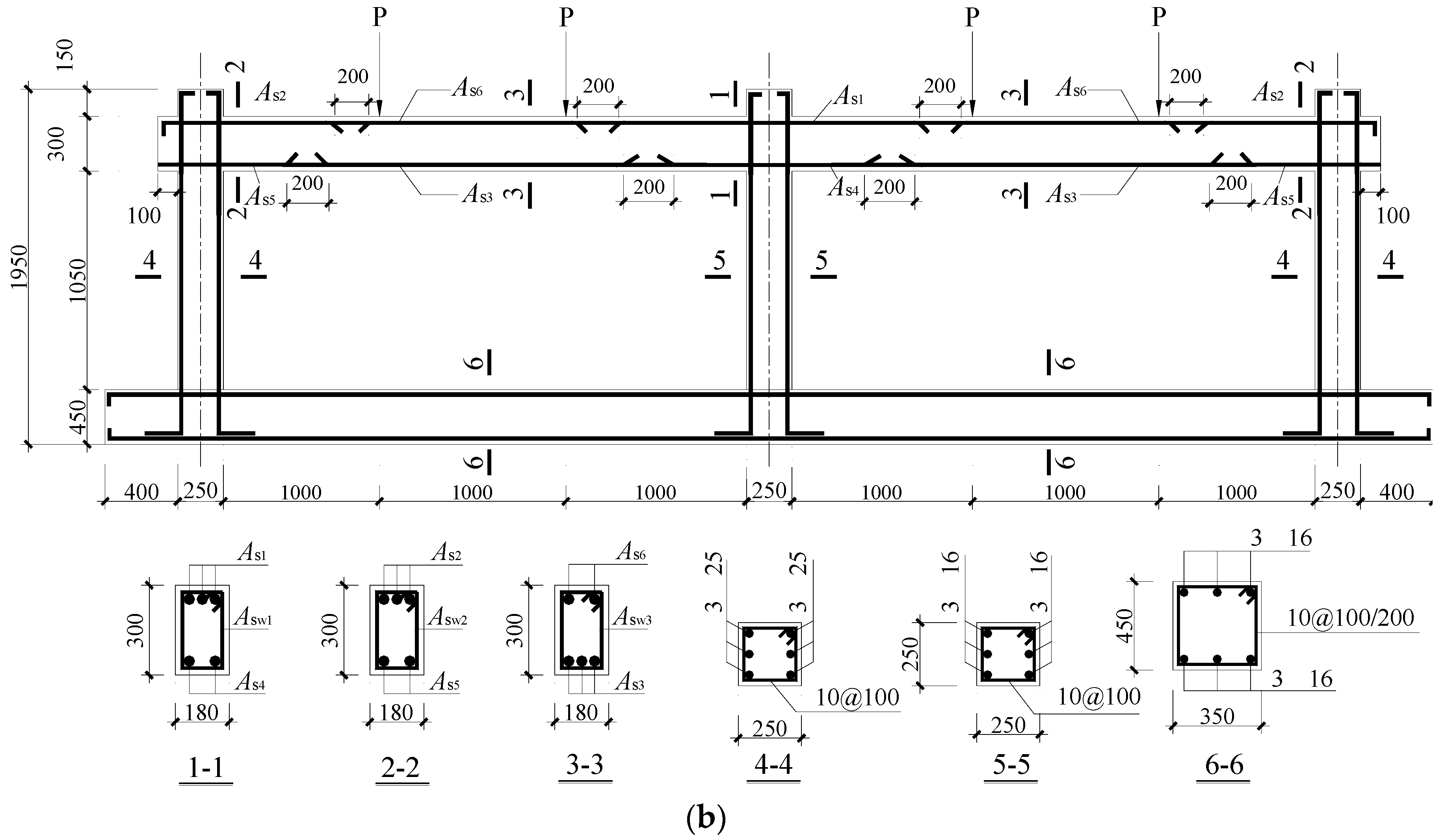
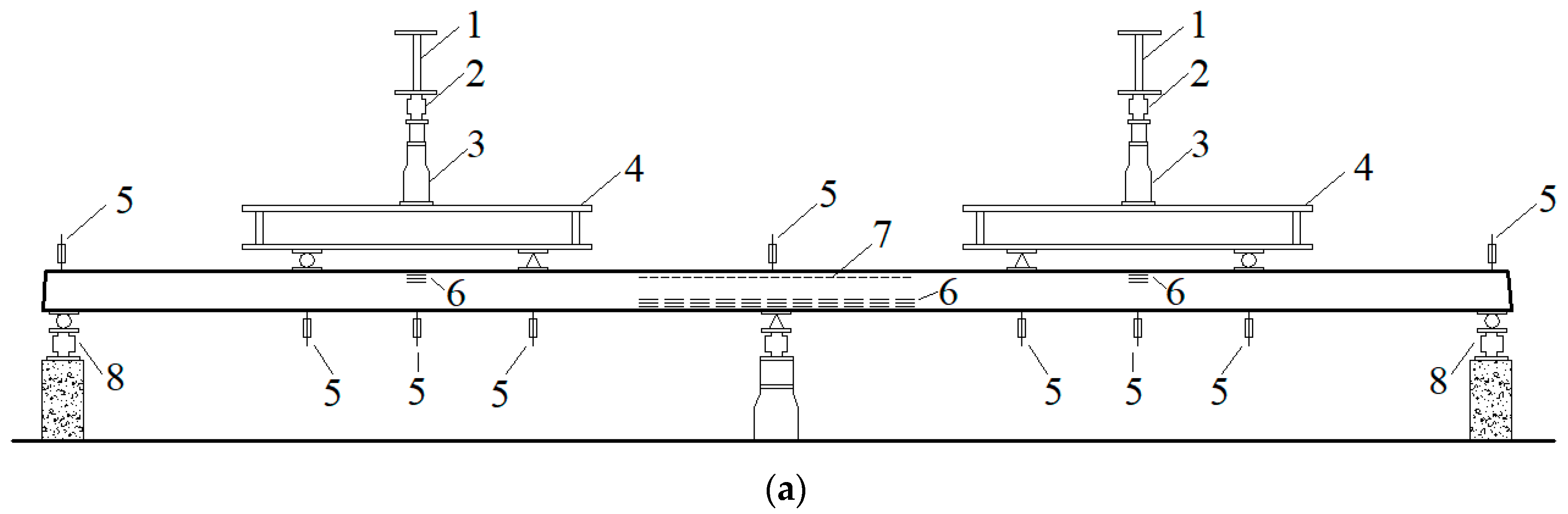
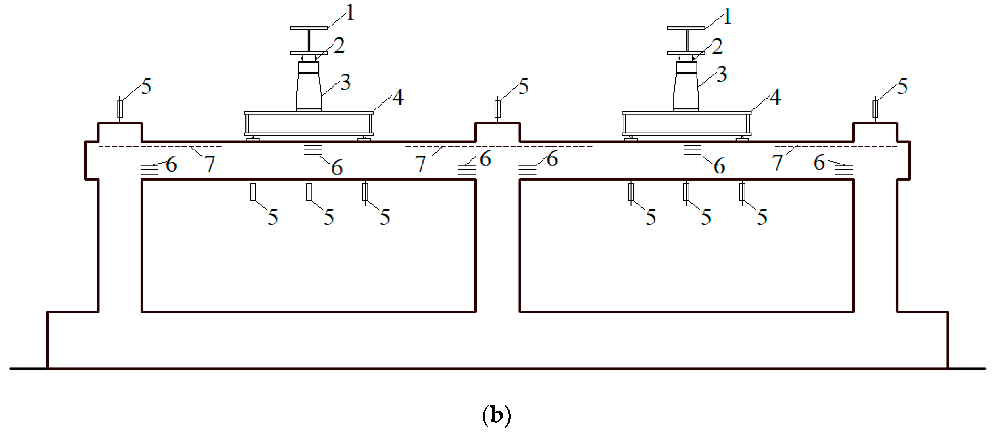
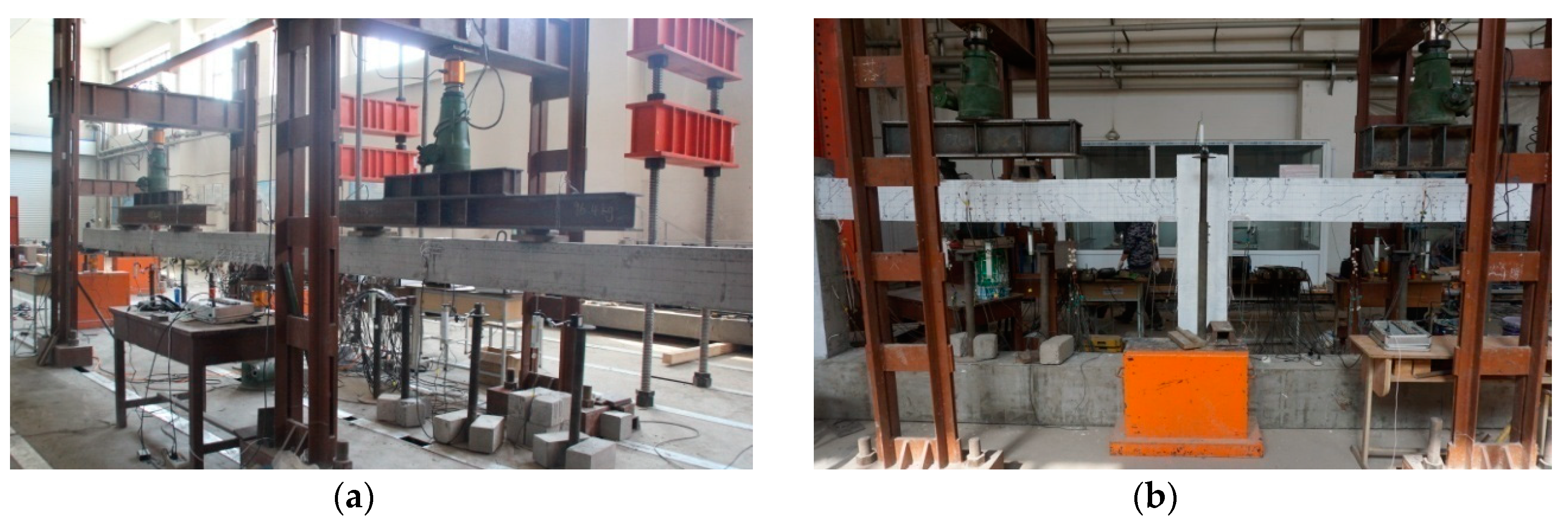
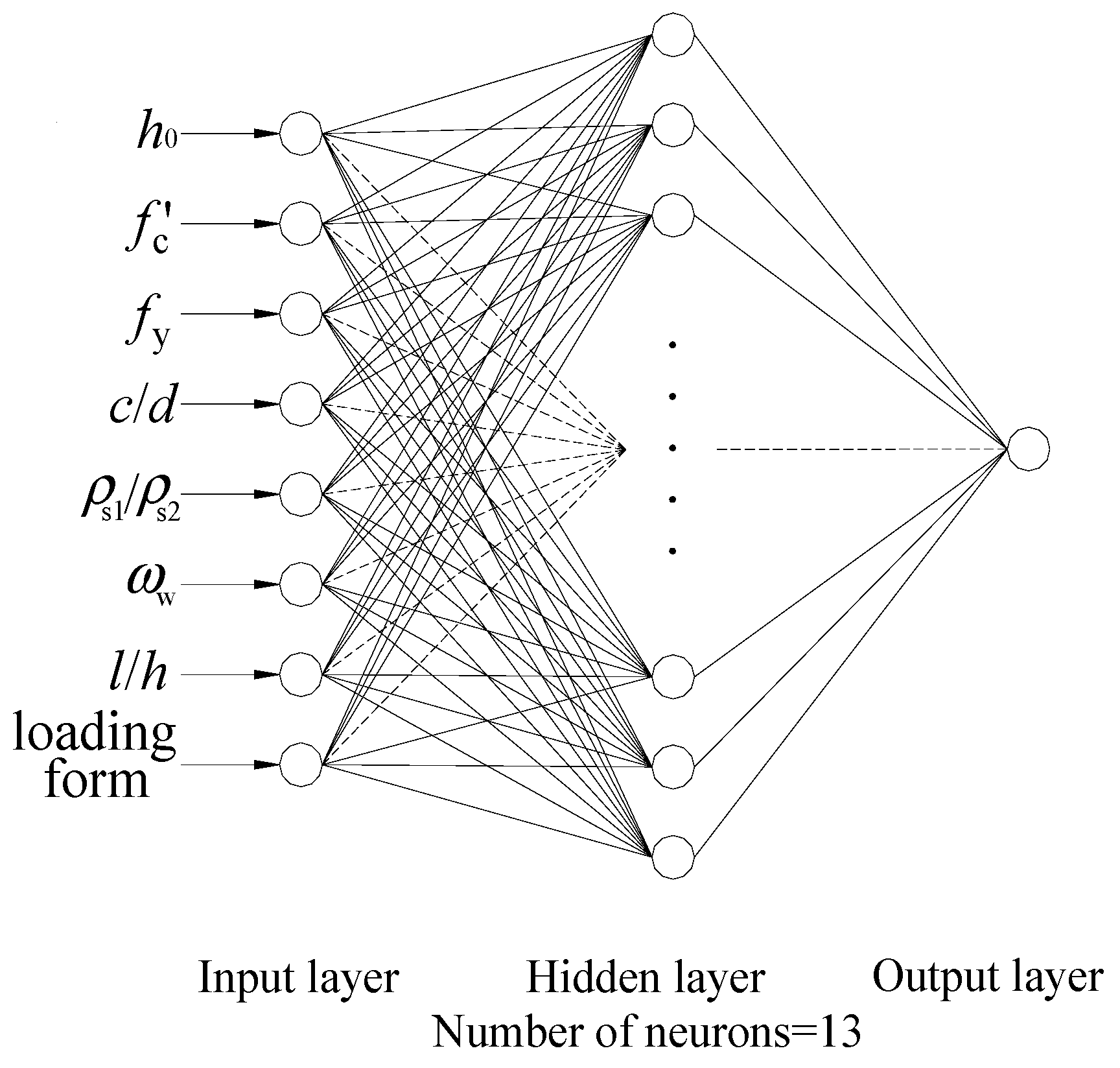
However, few studies have focused on the prediction of the moment redistribution in the statically indeterminate RC structures using artificial intelligence techniques. In this paper, an experimental study on the moment redistribution in 24 continuous RC beams and 12 continuous RC frames with various design parameters was presented. Furthermore, two models of ANN and SVM were developed using MATLAB software (MathWorks, Neddick, MA, USA) to predict the coefficient of moment redistribution in the statically RC indeterminate structures. In total, 111 experimental datasets were gathered to construct the models and a description of the development procedure is provided here. The main influential factors, including the neutral axis depth factor (c/d), the ratio of the tensile reinforcement ratio over the critical negative moment regions to the tensile reinforcement ratio over the positive moment regions (ρ_s1/ρ_s2), the yield strength of the reinforcement (f_y), the concrete compressive strength (f_c’), the slenderness ratio (l/h), the effective depth of the section (h₀), the stirrup ratio (ω_w), and the loading form, were used as input parameters to the models. Finally, the new proposed models were verified against the experimental results and compared with the provisions in the design codes to assess their accuracy and reliability.

2. Experimental Database

As the first step in developing the ANN and SVR models, a comprehensive set of experimental data on the moment redistribution was required for the training and testing samples. The database used in this paper was established by collecting the datasets from the experiments conducted in the current test and the relevant experimental programs in previous studies [3,6,7,33,34,35,36,37].

2.1. Experimental Program

2.1.1. Test Scheme

A total of 24 two-span continuous RC beams and 12 single-layer two-span continuous RC frames were designed and tested to investigate the moment redistribution at the negative moment regions. The rectangular cross-section of the continuous beams and frame beams were 180 mm × 250 mm and 180 mm × 300 mm, respectively. The length of each span of the continuous beams and frame beams are 4 m and 3 m, respectively. Owing to the limited number of test specimens, four main variables affecting the moment redistribution were considered in the design, namely, the neutral axis depth factor (c/d), the ratio of the tensile reinforcement ratio over the critical negative moment regions to the tensile reinforcement ratio over the positive moment regions (ρ_s1/ρ_s2), the yield strength of the reinforcement (f_y), and the concrete compressive strength (f_c’). All beams were designed to have a reserve capacity in the positive moment regions, which ensure that the internal forces transfer from the negative moment regions to the positive moment regions. A sufficient magnitude of stirrups was arranged in all beams to avoid shear failure, and the strong column–weak beam requirement was followed in the design of the frames. The mechanical properties of the tensile longitudinal reinforcements in the test specimens were measured by uniaxial tensile tests of the steel bars. The grades of the steel bars included HRB500 and HRB600 as specified in the Chinese code for design of concrete structures GB 50010-2010 [38].

Table 1. Mechanical properties of steel bars.

Grade	Diameter db	In Continuous RC Beams				In Continuous RC Frames
		fy(MPa)	εsy	fu(MPa)	εsu	fy(MPa)	εsy	fu(MPa)	εsu
HRB500	10	680	0.003400	850	0.120	—	—	—	—
	12	—	—	—	—	704	0.003520	880	0.122
	14	651	0.003255	814	0.112	817	0.004085	1022	0.131
	16	638	0.003190	830	0.115	—	—	—	—
	18	633	0.003165	823	0.113	631	0.003155	825	0.118
	20	633	0.003165	825	0.113	654	0.003270	837	0.114
	22	612	0.003060	800	0.108	618	0.003090	801	0.117
HRB600	14	540	0.002700	702	0.110	569	0.002845	710	0.110
	16	555	0.002775	723	0.115	555	0.002775	700	0.108
	18	533	0.002665	705	0.112	590	0.002950	760	0.116
	20	555	0.002775	713	0.114	581	0.002905	732	0.122
	22	555	0.002775	716	0.118	543	0.002715	713	0.113

lists some important characteristics of the steel bars with various diameters: yield strength f_y, yield strain ε_sy, ultimate tensile strength f_u, and ultimate strain ε_su. It should be noted that, since the steel bars in the test beams and the test frames were in different batches, there were some slight differences in the performance of the corresponding steel bars. The concrete compressive strength f_c’ was obtained from the compression tests of the concrete cylinders, which were prepared and cured in the same manner as the test specimens.

Table 2. Details of 24 continuous beams.

Specimens No.	fc’ (MPa)	Mid-Support Region				Mid-Span Region		ρs1/ρs2	l/d
		c/d	As1 (mm2)	fy (MPa)	ωsw1 (%)	As2 (mm2)	fy (MPa)
L-A-1	38.4	0.09	157	680	0.44	402	638	0.39	19.07
L-A-2	38.4	0.20	509	633	0.58	763	632	0.67	19.19
L-A-3	38.4	0.30	763	633	1.09	1008	620	0.76	19.30
L-A-4	38.4	0.39	1008	625	1.09	1074	620	0.94	19.42
L-A-5	46.4	0.10	236	680	0.44	461	638	0.51	19.07
L-A-6	46.4	0.21	628	633	0.87	942	633	0.59	19.19
L-A-7	46.4	0.31	942	633	1.74	1388	622	0.60	19.30
L-A-8	46.4	0.40	1140	612	1.74	1388	612	0.73	19.42
L-A-9	55.2	0.10	308	651	0.44	461	651	0.67	19.07
L-A-10	55.2	0.21	763	633	0.87	1140	612	0.67	19.19
L-A-11	55.2	0.31	1140	612	1.74	1520	612	0.66	19.30
L-A-12	55.2	0.36	1256	633	1.74	1140	633	1.00	19.88
L-B-1	37.6	0.12	308	540	0.44	461	540	0.67	19.07
L-B-2	36.0	0.22	603	555	0.87	942	555	0.64	19.19
L-B-3	38.4	0.33	942	555	1.09	1140	555	0.83	19.30
L-B-4	35.2	0.36	1017	555	0.87	942	555	1.08	19.42
L-B-5	37.6	0.12	308	540	0.44	461	540	0.67	19.07
L-B-6	37.6	0.25	763	533	0.87	1074	555	0.63	19.19
L-B-7	39.2	0.35	1140	555	1.74	1451	555	0.69	19.30
L-B-8	40.8	0.42	1256	555	1.74	1256	555	1.00	21.97
L-B-9	55.2	0.11	402	555	0.44	603	555	0.67	19.07
L-B-10	56.0	0.20	763	533	0.87	1256	555	0.61	19.19
L-B-11	56.0	0.27	1140	555	1.74	1702	555	0.59	19.30
L-B-12	56.8	0.34	1256	555	1.74	1391	555	0.90	21.97

Note. (1) This table should be read in conjunction with Figure 1a. (2) The bottom reinforcement in mid-support regions and the top reinforcement in mid-span regions were all 2T10 (157 mm²). (3) ω_sw1 presents the stirrup ratio in mid-support region. The steel bars with diameter of 10 mm are used as stirrups.

and

Table 3. Details of 12 frame beams.

Specimens No.	fc’ (MPa)	Mid-Support Region				End-Support Region				Mid-Span Region		ρs1/ρs3	ρs2/ρs3	l/d
		c/d	As1 (mm2)	fy (MPa)	ωsw1 (%)	c/d	As2 (mm2)	fy (MPa)	ωsw2 (%)	As3 (mm2)	fy (MPa)
KL-A-1	36.8	0.29	823	638	1.57	0.10	226	704	1.26	1140	618	0.72	0.20	11.54
KL-A-2	38.4	0.38	1140	618	2.51	0.17	461	817	1.57	1256	654	0.91	0.34	11.54
KL-A-3	50.4	0.27	1008	654	2.51	0.10	308	817	1.57	1140	618	0.82	0.25	11.54
KL-A-4	52.0	0.36	1256	654	2.51	0.13	461	817	2.51	1520	618	0.83	0.28	11.54
KL-A-5	54.4	0.28	1140	618	2.51	0.09	308	817	2.51	1388	636	0.82	0.20	11.54
KL-A-6	56.0	0.39	1520	618	2.51	0.13	509	631	2.51	1570	654	0.97	0.30	11.54
KL-B-1	35.2	0.32	942	581	1.57	0.10	308	569	1.26	942	581	1.00	0.33	11.54
KL-B-2	40.0	0.41	1256	581	2.51	0.15	509	590	1.57	1388	562	0.84	0.34	11.54
KL-B-3	50.4	0.26	1140	543	2.51	0.10	402	555	1.57	1388	562	0.82	0.29	11.54
KL-B-4	46.4	0.41	1520	543	2.51	0.13	509	590	2.51	1520	543	1.00	0.31	11.54
KL-B-5	47.2	0.38	1388	562	2.51	0.09	308	569	1.57	1388	562	0.92	0.20	11.54
KL-B-6	55.2	0.41	1702	581	2.51	0.14	628	590	2.51	2281	543	0.75	0.25	11.54

Note: (1) This table should be read in conjunction with Figure 1b. (2) The top reinforcement in mid-span regions, the bottom reinforcement in mid-support regions and end-support regions are all 2T10 (157 mm²). (3) ω_sw1 and ω_sw2 presents the stirrup ratio in mid-support and end-support region, respectively. The steel bars with diameter of 12 mm are used as stirrups.

list the details of the test specimens. Figure 1 presents the reinforcement arrangement of the specimens.

Each span of the test beams was subjected to two-point loads using hydraulic jacks via a loading distributed beam, as shown in Figure 2 and Figure 3. A force-controlled loading process was applied and the load increase rate was kept constant. Sensors were placed on each hydraulic jack so that the loads on each span were controlled to increase symmetrically. For the continuous beams, the reaction forces were measured with sensors under the three supports. For the frame beams, the inner forces were obtained by attaching strain gauges to the longitudinal reinforcement at the critical section of the top of the column. Then, the degree of moment distribution in the test specimens was achieved based on the above measurements continuously recorded during the loading process.

2.1.2. Test Results

Figure 4 shows the variation in the load with respect to the vertical displacement of some test continuous beams and frames in the loading process. Several characteristic points were observed during the loading process: crack formation at the negative moment regions (Point A or A’), crack formation at the positive moment regions (Point B), the yielding of the reinforcement (Point C or C’) and the crushing of the concrete at the negative moment regions (Point D or D’). For the frame beams, both the mid-support region and the end-support region were subjected negative moment, for which the characteristic states corresponded to Points A, C, and D and Points A’, C’, and D’ in Figure 4, respectively. It can be seen that the deflections of the east span beam and west span beam for the one specimen were largely symmetrical owing to their equal longitudinal steel ratios and symmetrically loading.

For the continuous beams, the moment redistribution of each beam was calculated based on the external loads P and the reaction forces measured by the sensors under the three supports. The evolution of the elastic reactions obtained by the elastic theory and the actual reactions obtained from the test are presented in relation to the external loads P, as shown in Figure 5 for specimen L-A-2. The characteristic points in the figure correspond to the four states mentioned above. It can be observed that the deviation between the actual reactions and the elastic reactions became increasingly obvious as the external load is increased, which indicates an increase in the moment redistribution of the test beams. Figure 6 shows the relationship between the coefficient of the moment redistribution and the actual moment at the support over the full load history of specimen L-A-2. For the continuous frame beams, the mid-support region and the end-support region of the frame beams were all subjected to the negative moment, from where the internal forces would transmit to the positive moment regions. Therefore, it can be approximately regarded as two processes of moment redistribution at the same time for each span of the frame beams and two coefficients of moment redistribution can be achieved. Similar to the continuous beams, the variation in the moment redistribution at both the mid-support and end-support for the test specimen KL-B-4 is depicted in Figure 6. The test results confirmed that the moment redistribution behavior occurs from the concrete crack (Point A or A’) and increases sharply after the yielding of the reinforcement at the critical section (Point C or C’). According to Equation (1), the degrees of the moment redistribution in the test specimens are summarized in

Table 4. Moment redistribution for test specimens.

Specimens No.	${\mathit{M}}_{\mathbf{elast}} (\mathbf{KN}·\mathbf{m})$	${\mathit{M}}_{\mathbf{red}} (\mathbf{KN}·\mathbf{m})$	β (%)	Specimens No.	${\mathit{M}}_{\mathbf{elast}} (\mathbf{KN}·\mathbf{m})$	${\mathit{M}}_{\mathbf{red}} (\mathbf{KN}·\mathbf{m})$	β (%)
L-A-1	51.54	24.06	53.33	KL-A-1(E)	93.90	44.20	52.93
L-A-2	94.16	53.53	43.15	KL-A-1(M)	159.62	117.84	26.17
L-A-3	138.12	90.57	34.42	KL-A-2(E)	142.30	84.92	40.32
L-A-4	145.85	104.57	28.31	KL-A-2(M)	193.09	148.58	23.05
L-A-5	48.20	24.59	48.98	KL-A-3(E)	115.17	57.29	50.26
L-A-6	108.68	66.76	38.57	KL-A-3(M)	206.27	153.62	25.53
L-A-7	137.24	91.16	33.58	KL-A-4(E)	160.55	84.37	47.45
L-A-8	122.46	87.78	28.32	KL-A-4(M)	206.19	153.10	25.75
L-A-9	60.86	33.13	45.57	KL-A-5(E)	140.14	55.04	60.73
L-A-10	142.12	91.56	35.57	KL-A-5(M)	228.79	159.87	30.13
L-A-11	124.48	89.59	28.03	KL-A-6(E)	126.08	75.45	40.16
L-A-12	115.36	84.75	26.53	KL-A-6(M)	235.89	190.73	19.14
L-B-1	63.94	32.82	48.65	KL-B-1(E)	79.81	40.75	48.94
L-B-2	95.06	52.86	44.39	KL-B-1(M)	147.00	110.20	25.03
L-B-3	116.01	75.85	34.61	KL-B-2(E)	114.62	67.64	40.98
L-B-4	102.36	68.93	32.67	KL-B-2(M)	181.09	139.00	23.24
L-B-5	50.59	27.32	45.99	KL-B-3(E)	115.17	53.57	53.49
L-B-6	107.48	68.15	36.60	KL-B-3(M)	190.43	140.17	26.39
L-B-7	128.80	87.85	31.79	KL-B-4(E)	132.61	72.39	45.41
L-B-8	136.79	95.00	30.55	KL-B-4(M)	206.27	151.13	26.73
L-B-9	78.18	42.40	45.76	KL-B-5(E)	126.53	49.92	60.54
L-B-10	110.15	70.92	35.61	KL-B-5(M)	200.19	146.91	26.61
L-B-11	136.79	96.44	29.50	KL-B-6(E)	137.60	89.67	34.83
L-B-12	124.79	85.26	31.68	KL-B-6(M)	225.61	189.98	15.79

Note: The letters E and M in the “specimens No.”, respectively, indicate the end-support and mid-support of the frame beams.

.

2.2. Data Collection

To comprehensively investigate the factors influencing the moment redistribution and make the proposed models more applicable, 63 test datasets were gathered from the literature [3,6,7,34,35,36,37,38] for expanding the database, as listed in

Table 5. Experimental datasets collected from the literature.

Specimens No.	h0	fc’	fy	c/d	ρs1/ρs2	ωw (%)	l/h	Loading Form	β	Ref.
1	370	22.56	493	0.14	1.00	0.34	5.40	Single point	0.282	[33]
2	370	20.08	486	0.12	1.00	0.34	5.40	Single point	0.289	[33]
3	370	21.92	495	0.12	1.00	0.34	5.40	Single point	0.304	[33]
4	220	36.40	545	0.11	0.25	0.34	10.42	Single point	0.560	[3]
5	220	36.40	565	0.16	0.36	0.34	10.42	Single point	0.480	[3]
6	220	36.40	560	0.28	0.64	0.34	10.42	Single point	0.210	[3]
7	220	36.40	557	0.43	1.00	0.34	10.42	Single point	0.180	[3]
8	220	36.40	565	0.16	0.36	0.67	10.42	Single point	0.510	[3]
9	220	36.40	560	0.28	0.64	0.67	10.42	Single point	0.250	[3]
10	220	36.40	557	0.43	1.00	0.67	10.42	Single point	0.100	[3]
11	220	73.80	536	0.03	0.16	0.34	10.42	Single point	0.570	[3]
12	220	73.80	565	0.08	0.36	0.34	10.42	Single point	0.390	[3]
13	220	73.80	560	0.14	0.64	0.34	10.42	Single point	0.290	[3]
14	200	76.40	569	0.07	0.41	0.84	13.41	Single point	0.388	[6]
15	200	70.90	569	0.15	0.82	0.84	13.41	Single point	0.158	[6]
16	200	69.50	569	0.22	0.81	0.84	13.41	Single point	0.351	[6]
17	200	73.20	569	0.29	0.74	0.84	13.41	Single point	0.105	[6]
18	200	84.00	569	0.33	0.94	0.84	13.41	Single point	0.054	[6]
19	200	132.46	563	0.18	1.00	0.29	11.36	Single point	0.250	[34]
20	200	104.46	565	0.17	0.68	0.29	11.36	Single point	0.318	[34]
21	200	102.31	571	0.13	0.54	0.29	11.36	Single point	0.453	[34]
22	270	28.86	530	0.39	0.62	0.90	13.33	Single point	0.065	[35]
23	270	28.86	530	0.58	0.94	0.90	13.33	Single point	0.060	[35]
24	270	30.78	545	0.23	0.50	0.90	13.33	Single point	0.076	[35]
25	270	30.78	545	0.51	1.00	0.90	13.33	Single point	0.113	[35]
26	270	28.86	545	0.38	0.60	0.90	13.33	Single point	0.065	[35]
27	270	30.78	537	0.30	0.64	0.90	13.33	Single point	0.076	[35]
28	370	21.68	515	0.13	1.00	0.34	6.25	Single point	0.183	[36]
29	370	22.16	567	0.22	1.00	0.51	6.25	Single point	0.150	[36]
30	370	15.44	550	0.37	1.00	0.63	6.25	Single point	0.156	[36]
31	370	22.16	567	0.32	1.00	0.72	6.25	Single point	0.144	[36]
32	370	18.96	543	0.46	1.00	0.84	6.25	Single point	0.110	[36]
33	270	25.40	427	0.11	1.00	0.90	10.00	Single point	0.352	[37]
34	270	25.40	564	0.31	1.00	0.90	10.00	Single point	0.076	[37]
35	270	25.40	339	0.13	1.00	0.90	10.00	Single point	0.413	[37]
36	270	25.40	339	0.13	1.00	0.90	10.00	Single point	0.423	[37]
37	270	25.40	339	0.13	1.00	0.90	10.00	Single point	0.421	[37]
38	270	26.50	339	0.13	1.00	1.10	10.00	Single point	0.401	[37]
39	270	26.50	339	0.13	1.00	1.30	10.00	Single point	0.448	[37]
40	270	34.60	339	0.10	1.00	0.90	10.00	Single point	0.411	[37]
41	270	38.90	339	0.09	1.00	0.90	10.00	Single point	0.444	[37]
42	270	55.60	339	0.06	1.00	0.90	10.00	Single point	0.441	[37]
43	220	41.44	607	0.18	0.64	0.26	11.07	Single point	0.370	[7]
44	220	41.44	449	0.12	0.60	0.26	11.07	Single point	0.320	[7]
45	220	96.32	541	0.07	0.67	0.26	11.07	Single point	0.380	[7]
46	220	96.32	449	0.05	0.60	0.26	11.07	Single point	0.340	[7]
47	120	41.44	541	0.30	0.67	0.19	20.29	Single point	0.230	[7]
48	120	41.44	607	0.32	0.64	0.19	20.29	Single point	0.320	[7]
49	120	41.44	449	0.22	0.60	0.19	20.29	Single point	0.270	[7]
50	120	41.44	449	0.09	0.67	0.19	20.29	Single point	0.380	[7]
51	120	41.44	449	0.09	0.67	0.19	20.29	Single point	0.340	[7]
52	120	41.44	449	0.09	0.70	0.19	20.29	Single point	0.260	[7]
53	120	41.44	539	0.12	0.74	0.19	20.29	Single point	0.220	[7]
54	120	96.32	449	0.04	0.67	0.19	20.29	Single point	0.400	[7]
55	120	41.44	539	0.05	0.75	0.19	20.29	Single point	0.390	[7]
56	120	41.44	497	0.10	0.67	0.19	20.29	Single point	0.250	[7]
57	120	41.44	541	0.11	0.70	0.19	20.29	Single point	0.320	[7]
58	120	41.44	541	0.12	0.74	0.19	20.29	Single point	0.270	[7]
59	220	41.44	541	0.25	1.14	0.26	11.07	Single point	0.130	[7]
60	220	41.44	449	0.20	1.09	0.26	11.07	Single point	0.200	[7]
61	120	41.44	449	0.06	0.41	0.19	20.29	Single point	0.500	[7]
62	120	96.32	449	0.04	0.67	0.19	20.29	Single point	0.450	[7]
63	220	96.32	541	0.07	0.67	0.26	11.07	Single point	0.330	[7]

. This experimental information included design details, material properties, and the degree of the moment redistribution determined by the internal force of the experimental specimens. It should be noted that these datasets were selected randomly and there was no inclusion of any factitious choice. In total, 111 datasets were obtained to construct the artificial neural network (ANN) and support vector regression (SVR) models. According to the previous studies and existing models [1,2,3,4,5,6,7,8], the neutral axis depth factor (c/d), the ratio of the tensile reinforcement ratio over the critical negative moment regions to the tensile reinforcement ratio over the positive moment regions (ρ_s1/ρ_s2), the yield strength of the reinforcement (f_y), the concrete compressive strength (f_c’), the slenderness ratio (l/h), the effective depth of the section (h₀), the stirrup ratio (ω_w) and the loading form were selected as the main influential parameters for the moment redistribution.

Table 6. Range of parameters in the database.

Variable	h0	fc’	fy	c/d	ρs1/ρs2	ωw (%)	l/h	β
Minimum	120	15.44	339	0.03	0.16	0.19	5.40	0.05
Maximum	370	132.46	817	0.58	1.14	2.51	21.97	0.61
Mean	229.95	46.86	552.14	0.22	0.71	0.99	13.91	0.32

presents the range and distribution of the parameters in the database.

3. Modeling Method

3.1. Artificial Neural Networks

The ANN is an information processing system that simulates the structure and functional features of the biological nervous system. It consists of a large number of highly interconnected processing elements (neurons), and their inherent laws can be obtained by the training of the input parameters, which leads to a strong nonlinear mapping ability [39].

3.1.1. Neural Network Architecture

The multilayer feed-forward back propagation network (MFBPN), first proposed by Rumerlhar et al. in 1986 [40], is one of the most commonly used ANN methods due to its simple structure and strong plasticity. The MFBPN is composed of three main parts: an input layer, one or more hidden layers and an output layer. All neurons in each layer are connected to the neurons in the next layer by network weights and biases. The values of the neuron received from the lower layer are multiplied by the specific weights and then summed with the bias. The sum is processed by predefined activation functions and transferred to the next layer, as follows:

$$y_j=f(ne{t}_j)=f({\displaystyle \sum _{i=1}^n{w}_{ij}{x}_i+b_j})$$

(2)

where net_j is the weighted sum for the jth neuron, x_i is the input values of the ith neuron in the lower layer, w_ij is the weight between the ith neuron and the jth neuron, b_j is the bias value of the jth neuron and f is the activation function. In the present work, sigmoid activations were used in each layer.

The MFBPN algorithm consists of two stages: forward propagation and back propagation, as depicted in Figure 7. It can be seen that, in the forward propagation process, each layer is organized in the forward direction and the input values are calculated by Equation (2), transferred from the input layer to the hidden layer and then to the output layer. The predicted values are compared with the experimental values. If the error does not satisfied the predetermined accuracy, the process reverses into the back propagation process. In the back propagation process, the error information is returned from the output layer to the input layer and the connection weights and biases values between the neurons in each layer are modified. This training process is repeated until the error reaches the desired requirement. There are many training algorithms for the back propagation network, including the gradient descent algorithm, Levenberg–Marquardt algorithm, and Bayesian regularization [40]. Among these, the Levenberg–Marquardt algorithm is considered the most efficient in terms of model prediction efficiency and accuracy [41], which was selected for the back propagation training in this investigation.

3.1.2. Construction of Neural Network

In this study, the collected experimental data of the moment redistribution coefficient were randomly divided into a training set and a testing set. Since the purposes in different experimental studies are diverse and the test programs are time-consuming and costly, datasets with complete variable information collected from the published literature are relatively few. To improve the applicability and generalization of the training model, 85% of the data were selected as training data, which were used to fit the parameters of the neural network, such as the weights and the bias in each layer. The remaining 15% of the data were used as testing data, which were independent of the training process and used to test the accuracy and applicability of the trained model.

The performance of the neural network models can be evaluated by two indexes: mean squared error (MSE) and coefficient of correlation (R²), as given by Equations (3) and (4):

$$\mathrm{MSE}=\frac{1}{n}{\displaystyle \sum _{i=1}^n{(t_i-c_i)}^2}$$

(3)

$$R^2=1-\frac{{\displaystyle \sum _{i=1}^n{(t_i-c_i)}^2}}{{\displaystyle \sum _{i=1}^n{(t_i-\overline{t})}^2}}$$

(4)

where n is the total number of the data, c_i and t_i are the predicted value and the target value of the ith data, and $\overline{t}$ is the average of the target values. A prediction model is considered to be better fitting when MSE and R² are closer to 0 and 1, respectively.

Eight nodes were used in the input layer because there were eight influential parameters for the moment redistribution studied. Before training the input data, normalizations for the input and target data should be performed since the sigmoid activation function is sensitive to the variations between 0 and 1. In this way, the stability and convergence rate of the training process can be improved. A linear relationship was used to scale the data from 0.1 to 0.9, given by Equation (5):

$$x_{i,\mathrm{scaled}}=(0.9-0.1)\times \frac{x_i-x_{\min }}{x_{\max }-x_{\min }}+0.1$$

(5)

where x_i,scaled is the normalized value, x_i is the value of the variable, and x_min and x_max are the minimum and maximum values of the variable, respectively.

The function of the hidden layer is to determine the inherent relationship between the input and output layers based on the training of the data. One hidden layer was used in the present neural network. The number of the nodes in the hidden layer is of great importance to the design of the neural network. An excessive number of the nodes results in an extension of the training time and the over-fitting of the data, which decreases the computational efficiency. However, if the number of the nodes is not enough, insufficient information leads to a decrease in the computational accuracy. Currently, there are no general rules to exactly determine the number of nodes. It is often based on experience, and the optimum result is obtained through trial and error. In this study, the number of the nodes in the hidden layer was selected from 6 to 15. Figure 8 and Figure 9 show the regression values and MSE of the neural network with different numbers of nodes. It can be seen that the model is optimal when 13 nodes were used in the hidden layer. Hence, the final network configuration used in present study is illustrated in Figure 10 and the values of the parameters for the neural network were determined as follows:

• Number of input layer units = 8
• Number of hidden layer units = 13
• Number of output layer units = 1
• Momentum rate = 0.9
• Learning rate = 0.4
• Error after learning = 8 × 10⁻⁸
• Learning cycle = 20,000

The weight matrix from input layer to hidden layer:

$$[\mathrm{W}]=\left[\begin{array}{cccccccc}-0.9164& 1.4807& -0.2350& 0.7380& 0.5355& 1.7293& 0.5331& 0.9447\\ -1.1448& 0.1450& 0.8474& -1.1383& 0.2907& -0.0782& 0.9073& -0.1725\\ -1.1361& 0.7619& 1.2173& -0.1638& 0.7868& -0.4796& 0.6270& 0.3624\\ -0.4634& 0.9261& 0.2160& 1.4655& -0.6984& -0.3826& -0.4355& 0.7621\\ 1.1211& 0.2946& -0.3320& -0.2785& -1.3229& -0.5631& -1.2747& -1.0460\\ 0.0504& -0.2413& -1.4971& 0.2827& 0.7573& 0.4910& 1.2722& -0.6579\\ 0.6535& -0.1205& 0.9175& -0.3086& 0.9226& 0.6071& -0.6191& -0.8808\\ -0.4555& 0.7322& 0.0410& 0.4642& -0.5956& -0.1809& 1.0324& 0.1272\\ 0.0690& -0.1080& -0.4671& 0.1252& 0.6155& -1.5093& 0.6859& 0.9966\\ 1.1041& 1.0773& 0.2277& -0.3272& -0.5194& -0.8479& 0.3947& 0.0658\\ 0.0231& 1.0058& 1.6269& 0.7262& 0.8975& 1.1943& -0.7830& 0.9840\\ 1.0543& -0.5834& 0.7153& 0.9577& 0.0572& 0.3346& -0.7952& 0.4914\\ 1.0419& -0.5879& 0.8209& 0.1742& -0.4689& -1.3133& -0.4841& 1.2483\end{array}\right]$$

The bias value for hidden layer:

[b1]^T = [1.8206 1.5318 1.4769 0.3322 − 0.6058 0.9448 − 0.2012 0.0762 0.3039 1.0370 2.5586 1.7822 1.4689]

The weight matrix from hidden layer to output layer:

[W2] = [1.0278 − 0.6339 0.9911 − 0.9114 1.1020 − 0.7080 − 0.6638 0.1710 0.2638 − 0.6078 − 1.2464 − 0.1087 0.6158]

The bias value for output layer: [b2] = [0.6815]

3.2. Support Vector Machine

SVM is an intelligent algorithm first proposed by Boser et al. in 1992 for general classification problems [42]. It is based on the principle of structural risk minimization (SRM), which aims to minimize an upper bound on the expected risk rather than minimizing the error of the training samples. This gives SVM better generalization ability even for small sample learning [43]. Moreover, with the introduction of the ε-insensitive loss function by Vapink [44], SVM has been extended to deal with regression problems, also known as support vector regression (SVR).

3.2.1. Support Vector Regression

The principle of SVR is briefly introduced here. In SVR, the main goal is to obtain a function that differs at most ε from the actual targets for all training data, while being as flat as possible [45]. This means that our attention is no longer focused on the errors because small residuals are inevitable, but we focus on avoiding errors larger than a certain value. Suppose that the training data are given as {(x₁, y₁), (x₂, y₂), …, (x_n, y_n)}, where n is the number of the training datasets, x_i is the input vector and y_i is the output target value. Then, a function f (x) corresponding to the lowest expected risk is constructed, and the ε-insensitive loss function is expressed as:

$$L_{\epsilon }(y,f(x))=\max \{0,\left|y-f(x)\right|-\epsilon \},\epsilon >0$$

(6)

For the linear regression, function f(x) can be represented by

$$f(x)=\langle w,x\rangle +b$$

(7)

where $w\in {\mathrm{R}}^{\mathrm{n}}$ is the weight vector, determining the orientation of a discriminating plane, and $\mathrm{b}\in \mathrm{R}$ is the scalar threshold, determining the offset of the discriminating plane from the origin [16]. In terms of the nonlinear regression, the process proceeds with mapping of the data into a high feature dimension space through a non-linear mapping procedure, and then solving a linear regression in this high feature dimension space. Then, a nonlinear mapping Φ is introduced and can be expressed as:

$$f(x)=\langle w,\mathsf{\Phi }(x)\rangle +b$$

(8)

To ensure the flatness of Equation (8), a smaller value of w is required. In real problems, it is impossible for all data points to have an error lesser than ε for the one function. For this reason, the slack variables ξ_i and ξ_i^* are introduced. Therefore, the SVR can be formulated as an optimization problem:

$$\mathrm{Minimize} \frac{1}{2}{\Vert w\Vert }^2+C{\displaystyle \sum _{i=1}^n({\xi }_i+{\xi }_i^{\ast }}) \mathrm{subjected} \mathrm{to} \{\begin{array}{l}{y}_i-\langle \mathrm{w},\mathsf{\Phi }({\mathrm{x}}_i)\rangle -b\le \epsilon +{\xi }_i\\ \langle \mathrm{w},\mathsf{\Phi }({\mathrm{x}}_i)\rangle +b-y_i\le \epsilon +{\xi }_i^{\ast }\\ {\xi }_i,{\xi }_i^{\ast }\ge 0\end{array}$$

(9)

where C is the regularized constant specified by the user. It is defined as the penalty factor to indicate the trade-off between the flatness of the function and the empirical error.

The optimization problem in Equation (9) can be solved by introducing the Lagrangian multipliers ${\alpha }_i,{\alpha }_i^{\ast },{\eta }_i,{\eta }_i^{\ast }$ and the above optimization problem can be transformed into a dual quadratic programming problem:

$$\begin{array}{l}\mathrm{Maximizing}-\frac{1}{2}{\displaystyle \sum _{i=1}^n{\displaystyle \sum _{j=1}^n({\alpha }_i-{\alpha }_i^{\ast })({\alpha }_j-{\alpha }_j^{\ast })K(x_i,x_j)}-}\epsilon {\displaystyle \sum _{i=1}^n({\alpha }_i+{\alpha }_i^{\ast })+{\displaystyle \sum _{i=1}^n{y}_i({\alpha }_i-{\alpha }_i^{\ast })}}\\ \mathrm{Subjected} \mathrm{to} {\displaystyle \sum _{i=1}^n({\alpha }_i-{\alpha }_i^{\ast })}=0 \mathrm{and} {\alpha }_i,{\alpha }_i^{\ast }\in [0,C]\end{array}$$

(10)

where $K(x_i,x_j)=\mathsf{\Phi }({\mathrm{x}}_i)·\mathsf{\Phi }({\mathrm{x}}_j)$ is defined as the kernel function, which is an important analysis technique in SVR. The values of ${\alpha }_i$ and ${\alpha }_i^{\ast }$ can be obtained by solving Equation (10), and the function f(x) is finally written as:

$$f(x)={\displaystyle \sum _{i=1}^n({\alpha }_i-{\alpha }_i^{\ast })K(x_i,x_j)+b}$$

(11)

3.2.2. Construction of SVR Model

As discussed above, the SVR model is constructed by optimizing the ε-insensitive loss function, in which the parameter ε and the regularized constant C are the important optimization factors. Furthermore, the selection of the kernel function is also closely related to the SVR model performance. The commonly used kernel functions in the regression include the linear kernel function, polynomial kernel function, radial basis function (RBF), and sigmoid kernel function. Considering the infinite dimensional feature space corresponding to the RBF, the following RBF is adopted in this study:

$$K(x_i,x_j)=e^{-\frac{{\Vert x_i-x_j\Vert }^2}{{\sigma }^2}}=e^{-g{\Vert x_i-x_j\Vert }^2}$$

(12)

where σ indicates the smoothness of the derived function and g = 1/σ² is the key parameter of the RBF.

To select the optimal values of the parameters ε, C, and g involved in the SVR model, a grid search algorithm was used in the present study. The basic idea of the grid search algorithm is to try every possible value of the parameters in a certain space with a specified step distance, and the parameters that optimize the performance of the SVR model with the best accuracy can be derived based on the cross-validation [46]. The process of the algorithm is illustrated through a flowchart, as shown in Figure 11. Similar to the construction of the neural network in Section 3.1.2., the collected experimental data of the moment redistribution coefficient were divided into two sets (85% for training and 15% for testing) for SVR. To increase the efficiency of the SVR training, the input and target data were normalized within the range of 0.1 to 0.9, in accordance with Equation (5), before the training of the input data. Based on the grid search algorithm and a six-fold cross-validation, the values of the parameters for the SVR were determined as follows: ε = 0.01, C = 20, and g = 0.03.

4. Results and Discussion

4.1. Evaluation of Results

The ANN and SVR models developed in the present study were used to predict the coefficient of moment redistribution for statically indeterminate structures. The predicted values and experimental results of the two models for the training and testing sets are presented and compared in Figure 12 and Figure 13. It can be seen intuitively that the predicted values for the both models show good agreement with the experimental values. To further evaluate the performance of the developed models, four indices of accuracy were calculated for the training and testing sets: mean squared error (MSE), determination coefficient (R²), mean absolute percentage error (MAPE) and integral absolute error (IAE). MSE and R² are computed using Equations (3) and (4), respectively, and MAPE and IAE are correspondingly expressed as follows:

$$\mathrm{MAPE}=\frac{1}{n}{\displaystyle \sum _{i=1}^n\left|\frac{t_i-c_i}{t_i}\right|}$$

(13)

$$\mathrm{IAE}=\frac{{\displaystyle \sum _{i=1}^n{\left[{(c_i-t_i)}^2\right]}^{1/2}}}{{\displaystyle \sum _{i=1}^n{t}_i}}\times 100\%$$

(14)

All performance indices for the proposed ANN and SVR models are listed in

Table 7. Performance indices of ANN and SVR models.

Performance Indices	ANN		SVR
	Training	Testing	Training	Testing
MSE	0.0009	0.0009	0.0001	0.0008
MAPE	0.0989	0.0850	0.0079	0.0526
R2	0.9521	0.9431	0.9950	0.9485
IAE	0.0694	0.0813	0.0080	0.0538

, which indicates that both models have high-precision prediction ability for the coefficient of moment redistribution. Moreover, the SVR model showed slightly better results than the ANN model.

4.2. Comparison with the Different Provisions in Design Code

In most design codes, the permissible moment redistribution β can be calculated using the neutral axis depth factor c/d as a main parameter, as shown in Figure 14. It can be seen that the provisions for moment redistribution in various design codes are quite different, such as the upper bound of β, the limited range of c/d, and the divergence between the predictions. In addition, the amount of moment redistribution is not only related to c/d but also to the variation in the stiffness distribution and the bond between the reinforcement and concrete. However, the latter factors are usually not considered in design codes. The detailed provisions in the design codes are illustrated below.

In CSA A23.3-14 [47], the negative moments at the supports of continuous flexural members can be increased or decreased by:

$$\beta (\%)\le 30-50c/d$$

(15)

and β is no more than 20%.

In BS 8100-1:1997 [48], the neutral axis depth of the cross-section subjected to the largest moment should be checked by the expression with the permissible percentage of moment redistribution as an independent variable. In other words, β can also be treated as a function of c/d:

$$\beta \le 0.6-c/d$$

(16)

with a maximum of 0.3.

The AS 3600-2009 [49] indicates that the elastically determined bending moments at any interior support of statically indeterminate members with reinforcement of Ductility Class N (the uniform elongation is no less than 5.0% and the tensile-to yield stress ratio is no less than 1.08) may be reduced or increased by:

$$\beta (\%)=\{\begin{array}{ll}30\%& c/d\le 0.2\\ (30-75c/d)\%& 0.2<c/d\le 0.4\\ 0& c/d>0.4\end{array}$$

(17)

In the DIN 1045-1:2008 [50], fib Model Code 2010 [51] and EN 1992-1-1:2004 [52], the provisions for the moment redistribution are similar. The statically indeterminate members allowed for moment redistribution are predominantly subjected to flexure and the ratio of the adjacent spans is in the range of 0.5–2. Except for the neutral axis depth factor, the coefficient of the moment redistribution also depends on the ductility of reinforcement and concrete strength, as listed in

Table 8. Coefficient of moment redistribution in DIN1045-1:2008 [50], fib MC2010 [51] and EN 1992-1-1:2004 [52].

Code	Ductility of Reinforcement	Concrete Strength	Coefficient
DIN1045-1:2008 [50]	High ductility	Lower than C50/60	$\beta \le 0.36-0.8c/d\le 0.3$
		Higher than C55/67 and lightweight concrete	$\beta \le 0.28-0.8c/d\le 0.2$
	Normal ductility	Lower than C50/60	$\beta \le 0.36-0.8c/d\le 0.15$
		Higher than C55/67 and lightweight concrete	0
Fib Model Code 2010 [51] and EN 1992-1-1:2004 [52]	Class B, C or D	$f_{c^{\prime }}\le 50\mathrm{MPa}$	$\beta \le 0.56-1.25(0.6+0.0014/{\epsilon }_{\mathrm{c}u2})c/d\le 0.3$
		$f_{c^{\prime }}>50\mathrm{MPa}$	$\beta \le 0.64-1.25(0.6+0.0014/{\epsilon }_{\mathrm{c}u2})c/d\le 0.3$
	Class A	$f_{c^{\prime }}\le 50\mathrm{MPa}$	$\beta \le 0.56-1.25(0.6+0.0014/{\epsilon }_{\mathrm{c}u2})c/d\le 0.2$
		$f_{c^{\prime }}>50\mathrm{MPa}$	$\beta \le 0.64-1.25(0.6+0.0014/{\epsilon }_{\mathrm{c}u2})c/d\le 0.2$

Note: (1) The ductility of steel are defined by minimum specified values for the characteristic values of the tensile-to-yield stress ratio (f_t/f_y)_k and the strain at maximum stress ε_uk. In DIN1045-1, high ductility: ${(f_{\mathrm{t}}/f_{\mathrm{y}})}_{\mathrm{k}}\ge 1.08,{\epsilon }_{\mathrm{uk}}\ge 5.0\%$; normal ductility: ${(f_{\mathrm{t}}/f_{\mathrm{y}})}_{\mathrm{k}}\ge 1.05,{\epsilon }_{\mathrm{uk}}\ge 2.5\%$. In fib Model Code 2010 and EN 1992-1-1:2004, Class A: ${(f_{\mathrm{t}}/f_{\mathrm{y}})}_{\mathrm{k}}\ge 1.05,{\epsilon }_{\mathrm{uk}}\ge 2.0\%$; Class B: ${(f_{\mathrm{t}}/f_{\mathrm{y}})}_{\mathrm{k}}\ge 1.08,{\epsilon }_{\mathrm{uk}}\ge 5.0\%$; Class C: ${(f_{\mathrm{t}}/f_{\mathrm{y}})}_{\mathrm{k}}\ge 1.15 and \le 1.35,{\epsilon }_{\mathrm{uk}}\ge 7.5\%$; Class D:${(f_{\mathrm{t}}/f_{\mathrm{y}})}_{\mathrm{k}}\ge 1.25 and \le 1.45,{\epsilon }_{\mathrm{uk}}\ge 8.0\%$. (2) In DIN 1045-1, C50/60 presents the cylinder compressive strength $f_{c^{\prime }}\le 50\mathrm{MPa}$ and the cube compressive strength $f_{\mathrm{cube}}=60\mathrm{MPa}$; C55/67 presents $f_{c^{\prime }}=55\mathrm{MPa}$ and $f_{\mathrm{cube}}=67\mathrm{MPa}$. (3) In fib Model Code 2010 and EN 1992-1-1:2004, ${\epsilon }_{\mathrm{cu}2}$ is the concrete ultimate strain, for $f_{c^{\prime }}\le 50\mathrm{MPa}$, ${\epsilon }_{\mathrm{cu}2}(‰)=3.5$; for $f_{c^{\prime }}>50\mathrm{MPa}$, ${\epsilon }_{\mathrm{cu}2}(‰)=2.6+35{[(90-f_{c^{\prime }})/100]}^4$.

.

The ACI 318-14 [53] uses the net tensile strain ε_t as an indicator of the permissible moment redistribution, as given by:

$$\beta (\%)\le 1000{\epsilon }_{\mathrm{t}}\le 20\%$$

(18)

where ε_t is the tensile strain in the extreme layer of longitudinal tension steel at nominal strength, excluding strains due to effective prestress, creep, shrinkage and temperature and is required to be more than 0.75%.

Notably, the coefficient of the moment redistribution specified in the design codes are calibrated through a safe envelope formed from the available experimental data with a certain probability and not from the real values such as the database values used in the present study for constructing the models.

To study the performance of different approaches in design codes as well as the proposed ANN and SVR models, comparisons of their predicted results were conducted. Based on the database constructed in this study, as well as additional data points obtained from in literature [54], the ratios of the predicted results obtained from different methods (including the proposed methods and the provisions in the design codes) to the experimental results β_pre/β_exp are presented in Figure 15. It can be seen that most of the ratios β_pre/β_exp based on the design codes were plotted below a scale of 1.0.

Table 9. Comparisons between ANN, SVR models and methods specified in the design codes.

Method	Mean	COV	IAE
ANN	1.0335	0.1095	6.77%
SVR	0.9952	0.0549	2.42%
CSA A23.3-14 [47]	0.6141	0.6818	52.20%
BS 8100-1:1997 [48]	1.3474	0.6208	30.68%
AS 3600-2009 [49]	0.5834	0.7040	45.61%
DIN 1045-1:2008 [50]	1.0761	0.8328	39.61%
Fib Model Code 2010 [51] EN 1992-1-1:2004 [52]	0.7911	0.7496	38.55%
ACI 318-14 [53]	0.3485	0.8374	64.11%

summarizes the mean values, coefficient of variation (COV) and IAE of the ratio β_pre/β_exp for different methods. The comparison shows that clear differences exist among various design codes. The most liberal is the BS 8100-1:1997 [48], for which the mean value of the ratio β_pre/β_exp was 1.35, and the COV and IAE were 0.62 and 30.68%, respectively. The DIN 1045-1:2008 [50] was moderate with the ratio β_pre/β_exp of 1.08. Except for these two design codes, the mean values of the ratios based on the other design codes range from 0.35 to 0.79, and the COV and IAE are within the ranges of 0.68–0.84 and 38.55–64.11%, respectively. Despite the conservative nature of the code methods, the predicted values are significantly lower than the experimental results. These indicate the limitations and wide variations between national standards. Meanwhile, it can be known that the mean values of β_pre/β_exp for the ANN and SVR models were fairly close to 1.0, and the values of COV and IAE were very low. This indicates that the proposed models can estimate the coefficient of moment redistribution with sufficient precision. In addition, it can also be observed that the predicted results of the additional specimens outside the database agreed well with the experimental results, which demonstrates the applicability of the proposed models. In conclusion, the proposed ANN and SVR models can provide an approximate basis for the revision and unification of the moment redistribution provisions in the various codes due to their relative comprehensive consideration of the influential factors as well as their high accuracy.

5. Conclusions

An experimental study of 24 continuous RC beams and 12 continuous RC frames with various design parameters was performed to investigate the whole process of moment redistribution. Moreover, ANN and SVM models were established using MATLAB software (MathWorks, Neddick, MA, USA) for predicting the coefficient of the moment redistribution based on a reliable database with a total of 111 datasets, which was achieved using the experimental results in this study and the test data gathered from the published literature. The following conclusions can be drawn from the present study:

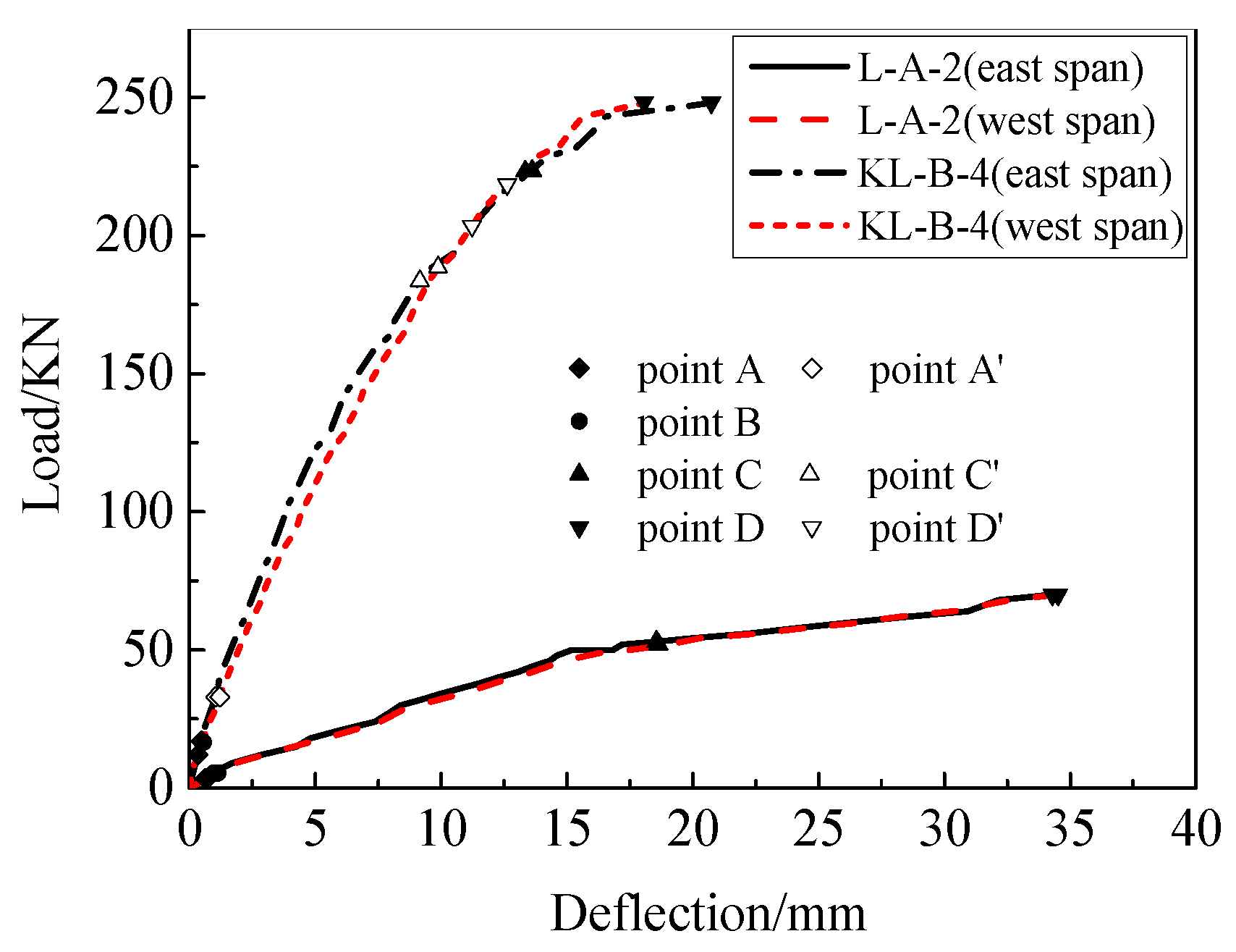
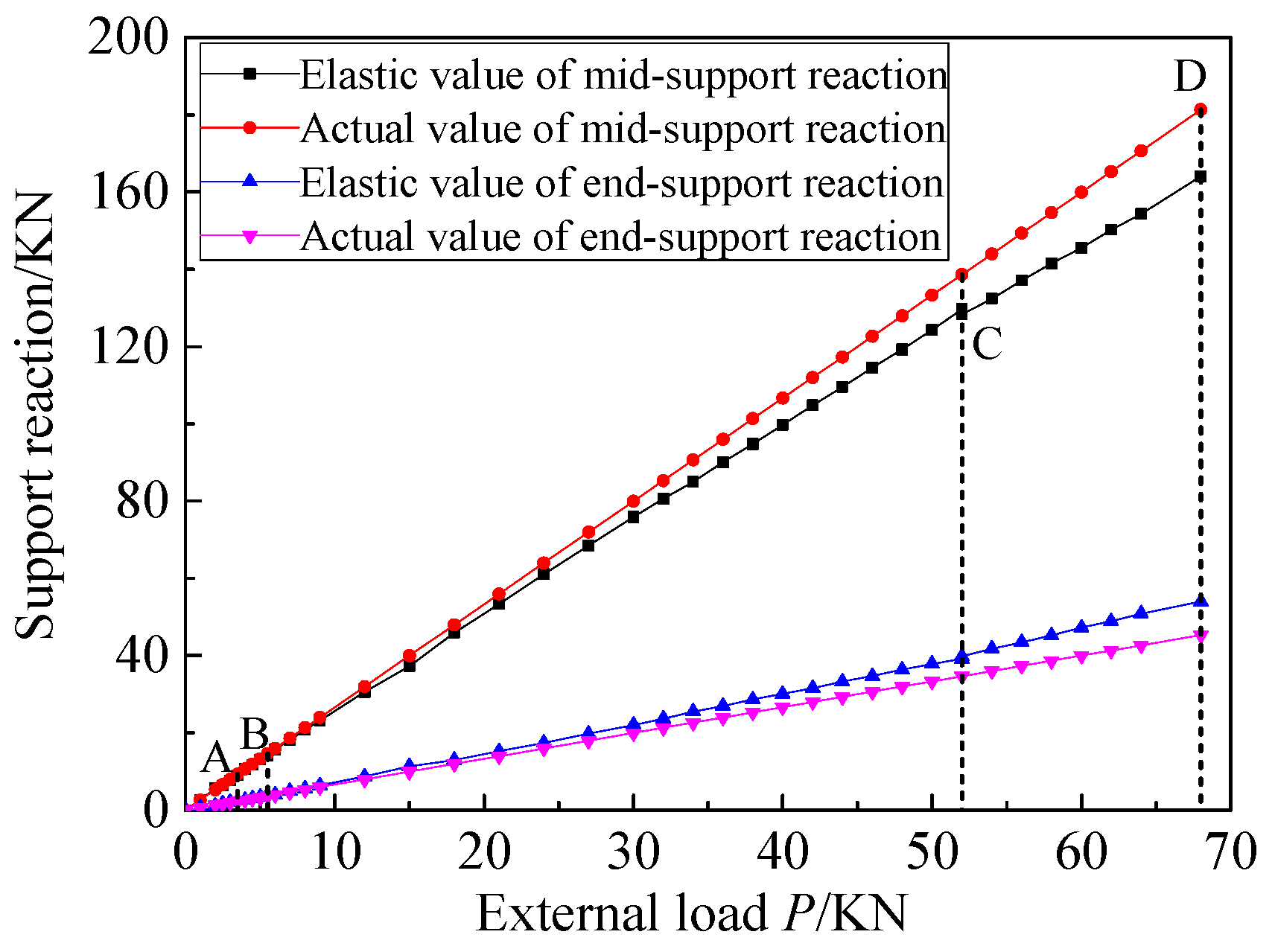
(1) In statically indeterminate RC structures, moment redistribution occurs during the whole loading process, beginning from the cracking of the concrete and increasing sharply after the yielding of the reinforcement at the critical section. Due to the complex process, the influential factors related to the material, structure and loading should be fully considered in the prediction models.

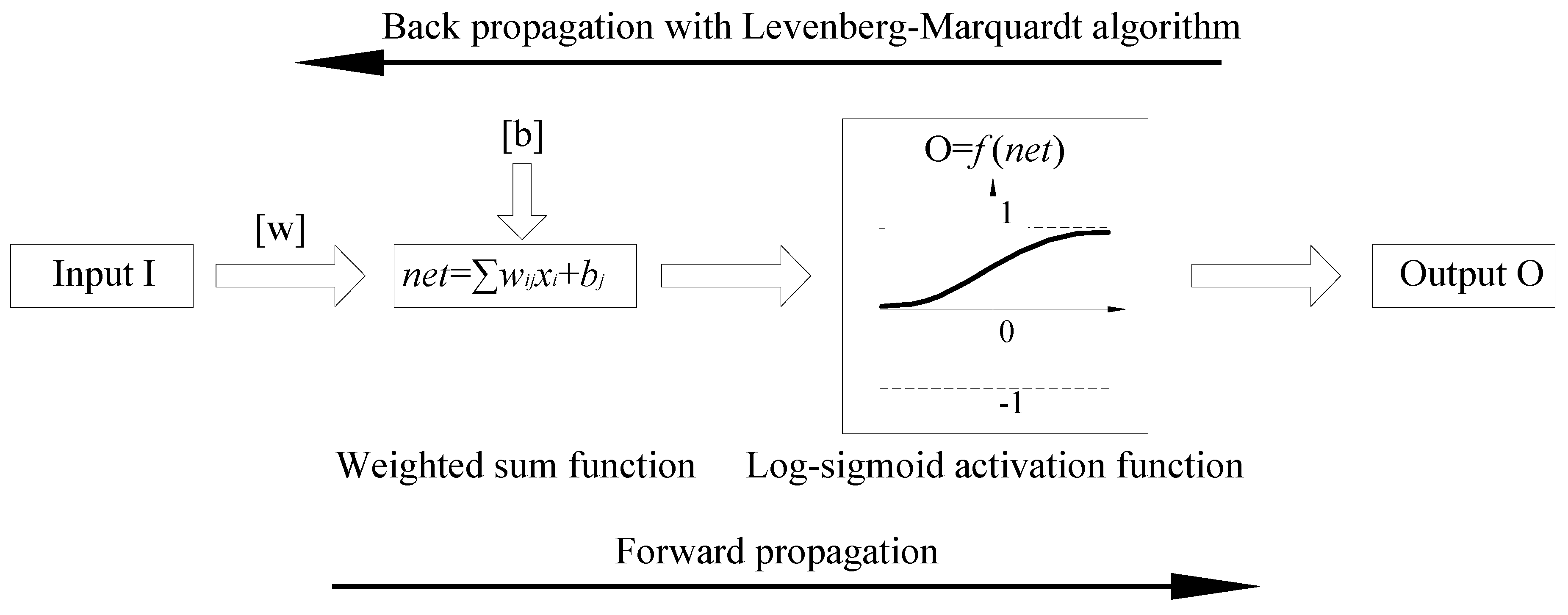
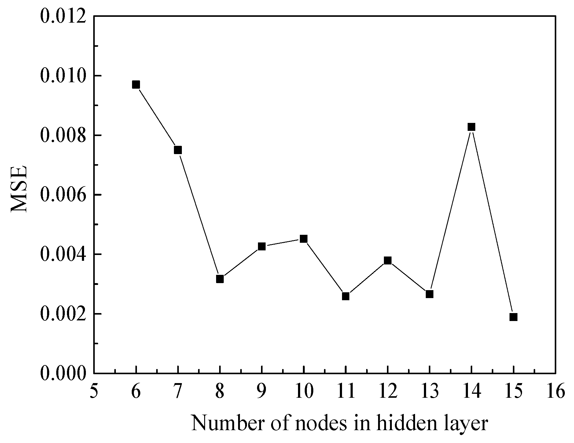
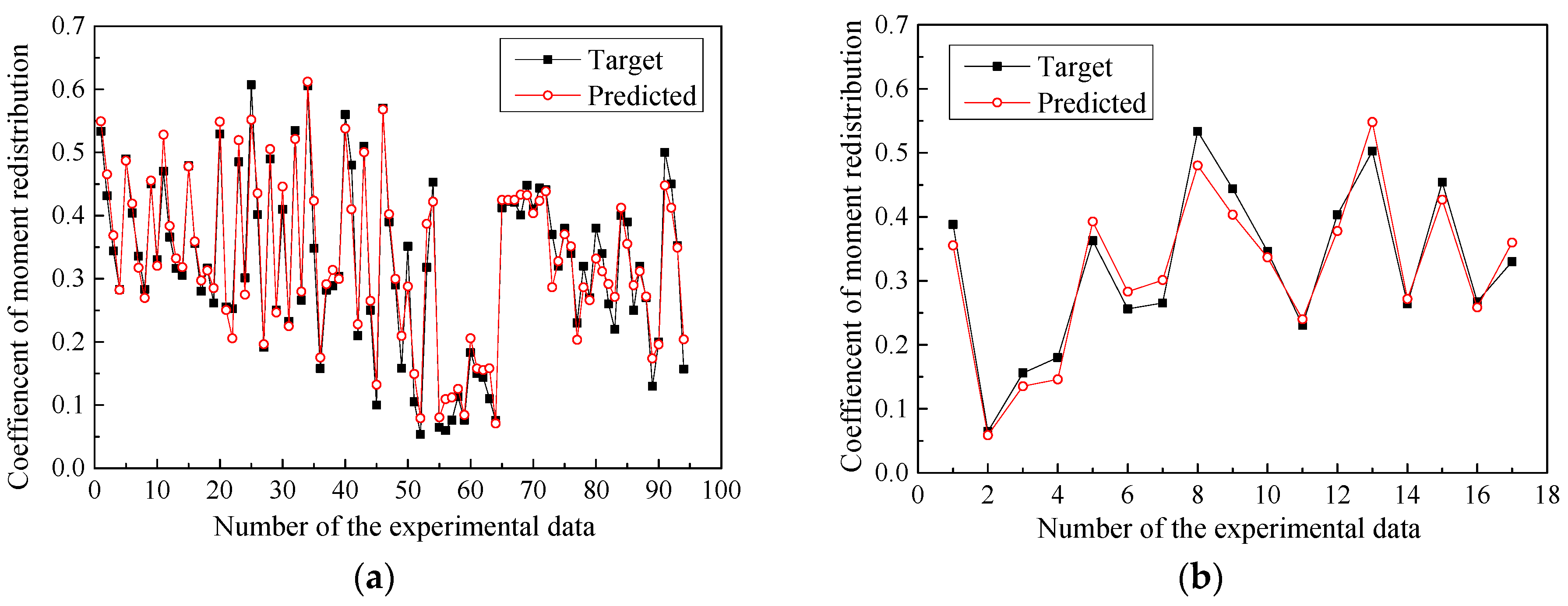
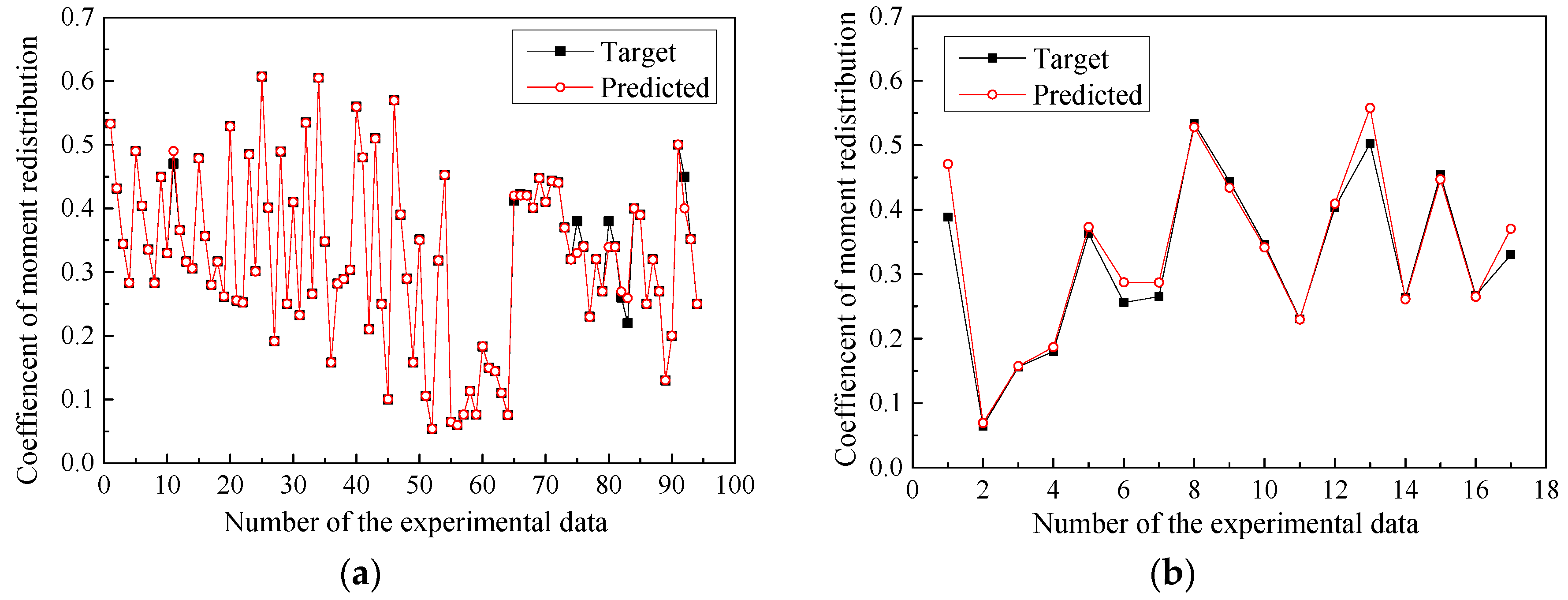
(2) Through a process of trial and error, a BP neural network model trained by the Levenberg–Marqardt (LM) algorithm, with 8 neurons in the input layer and 13 neurons in the hidden layer, was selected as being optimal for predicting the coefficient of the moment redistribution. The R² and MSE values for both the training and testing data were 0.95 and 0.0009, respectively, denoting that the proposed ANN models have high prediction accuracy.

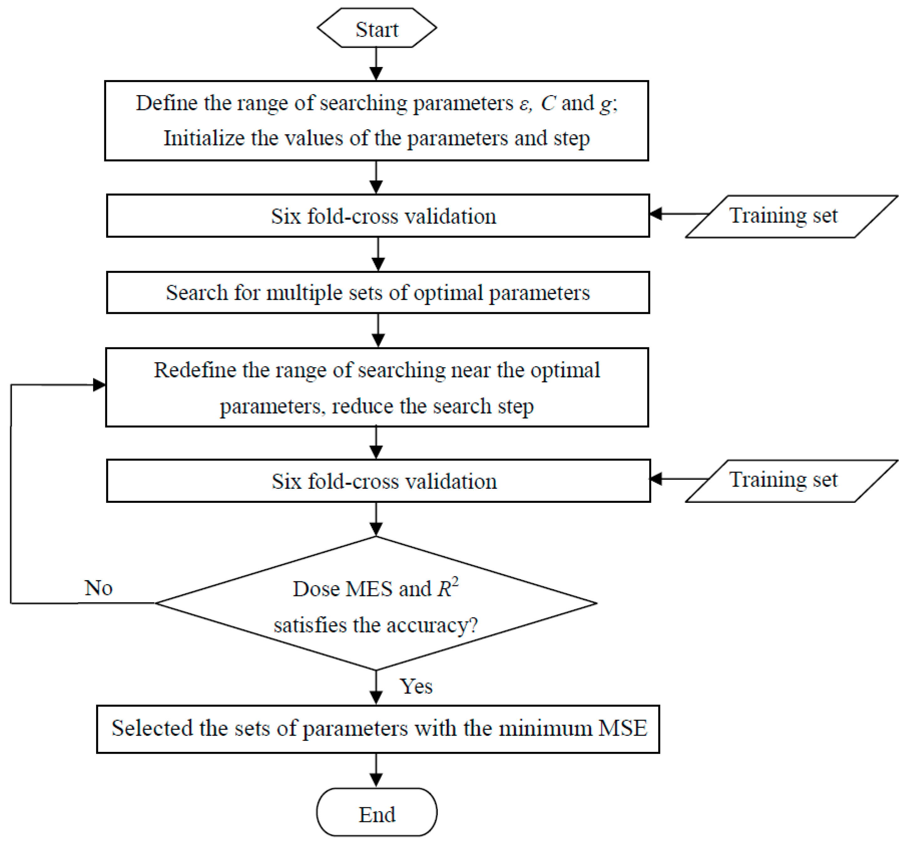
(3) Through a grid search algorithm, the values of the parameters involved in the SVR model were determined as ε = 0.01, C = 20, and g = 0.03. With RBF as the kernel function, the proposed SVR model exhibited good predictive performance. The values of R² for the training and testing data were 0.99 and 0.95, and the MSE values were 0.001 and 0.008, respectively. Moreover, the comparison of the performance indices showed that the accuracy of the SVR model is slightly higher than the ANN model for predicting the coefficient of the moment redistribution.

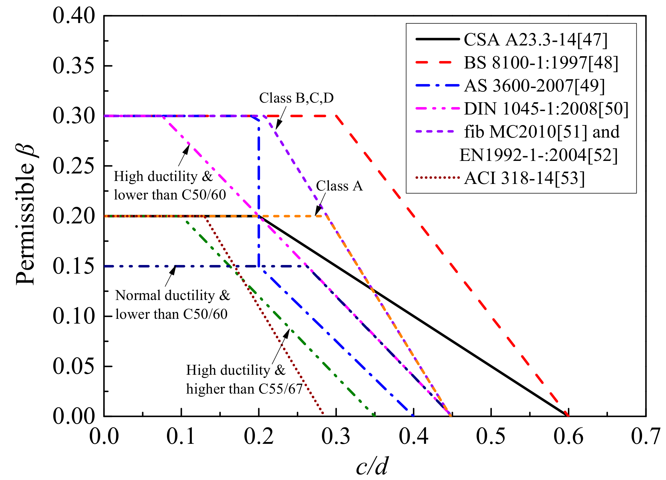
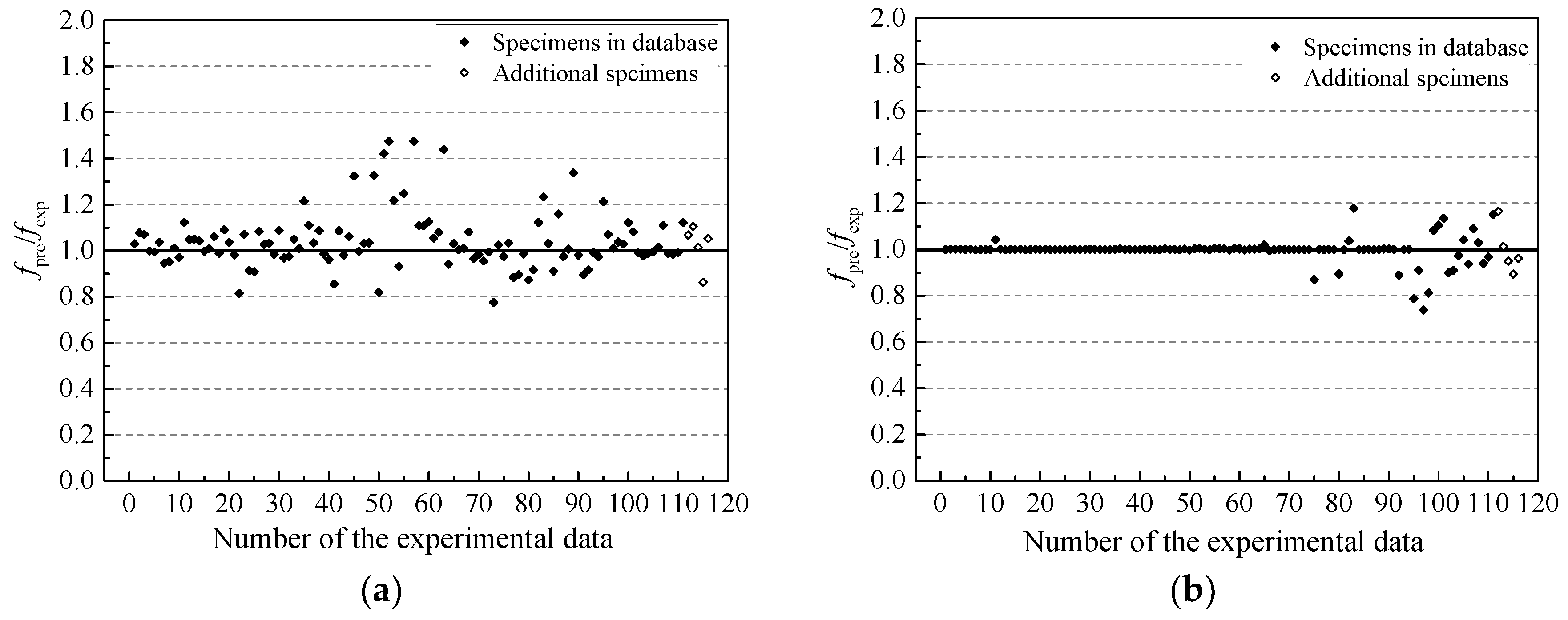
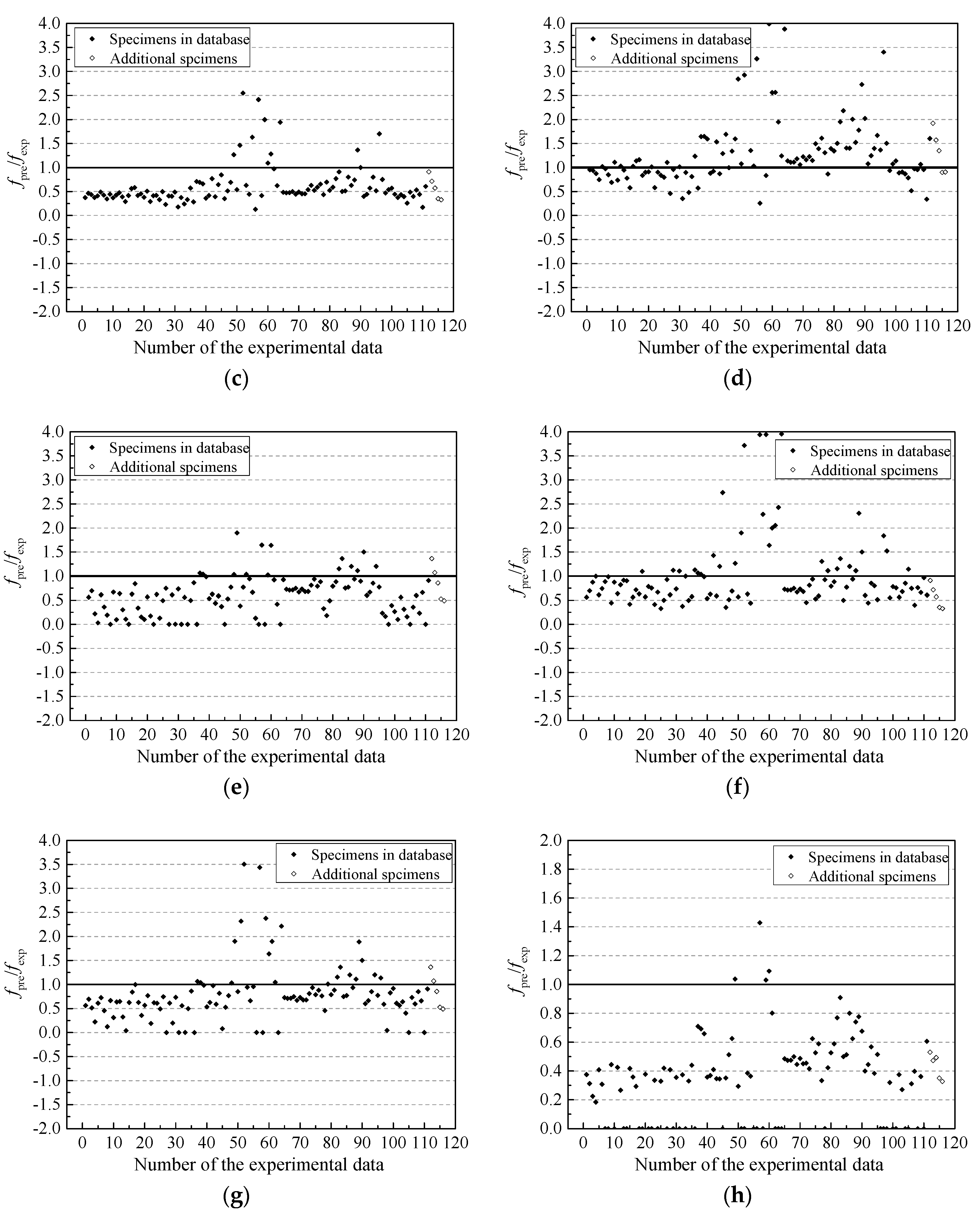
(4) Efficiencies of the ANN and SVR model were compared with six structural design codes. Despite the conservative nature of the code methods, most predicted values with the design code were significantly lower than experimental results since the range of the mean values and the COV for the ratio β_pre/β_exp were 0.35–1.35 and 0.62–0.84, respectively, whereas the mean values of β_pre/β_exp for the two proposed models were closer to 1.0 and the COV values of β_pre/β_exp were 0.11 and 0.05, respectively. The predicted values closely agreed with the experimental results.

ANN and SVR can be used as effective methods for the design of statically indeterminate RC structures because they can allow structural designers to accurately predict the degree of moment redistribution without conducting costly and time-consuming confirmatory experiments. Further parametric studies can be carried out to analyze the impacts of input parameters on moment redistribution to help the designers make more rational use of these parameters. Based on the large amount of results obtained from the models with respect to various input values, mathematical formulae with a certain safe guarantee rate can be established in future research, which may provide convenience for the application of the designers and references for the design codes.

Nevertheless, the developed models are valid within the range of variables investigated in this study and the local invariance of some input parameters may lead to slightly negative effects on the accuracy and modeling capability of the developed algorithms. Therefore, further experimental research is needed to expand the database and thereby increase the accuracy and applicability of the models.

References

1. Cohn, M.Z. Continuity in Prestressed Concrete. In Partial Prestressing, From Theory to Practice; Springer: Dordrecht, Netherlands, 1986. [Google Scholar]
2. Scholz, H. Ductility, redistribution, and hyperstatic moments in partially prestressed members. ACI Struct. J. 1990, 87, 341–349. [Google Scholar]
3. Bagge, N.; O’Connor, A.; Elfgren, L.; Pedersen, C. Moment redistribution in RC beams—A study of theinfluence of longitudinal and transverse reinforcement ratios and concrete strength. Eng. Struct. 2014, 80, 11–23. [Google Scholar] [CrossRef]
4. Scholz, H. Contribution to redistribution of moments in continuous reinforced concrete beams. ACI Struct. J. 1993, 90, 150–155. [Google Scholar]
5. Mostofinejad, D.; Farahbod, F. Parametric study on moment redistribution in continuous rc beams using ductility demand and ductility capacity concept. Iran. J. Ofence Technol. Trans. B Eng. 2007, 31, 459–471. [Google Scholar]
6. Carmo, R.N.F.D.; Lopes, S.M.R. Ductility and linear analysis with moment redistribution in reinforced. Can. J. Civil Eng. 2011, 32, 194–203. [Google Scholar] [CrossRef]
7. Scott, R.H.; Whittle, R.T. Moment redistribution effects in beams. Mag. Concr. Res. 2005, 57, 9–20. [Google Scholar] [CrossRef] [Green Version]
8. Oehlers, J.; Mohamed, D.A.; Haskett, M.; Griffith, M. Moment redistribution in reinforced concrete beams. Proc. ICE Struct. Build. 2010, 163, 165–176. [Google Scholar] [CrossRef]
9. Oehlers, D.J.; Ali, M.S.M.; Griffith, M.C. Concrete Component of the Rotational Ductility of Reinforced Concrete Flexural Members. Adv. Struct. Eng. 2008, 11, 281–291. [Google Scholar] [CrossRef]
10. Mohamed Ali, M.S.; Oehlers, D.J.; Griffith, M.C.; Seracino, R. Interfacial stress transfer of near surface-mounted FRP-to-concrete joints. Eng. Struct. 2008, 30, 1861–1868. [Google Scholar] [CrossRef]
11. Lou, T.; Lopes, S.M.R.; Lopes, A.V. FE modeling of inelastic behavior of reinforced high-strength concrete continuous beams. Struct. Eng. Mech. 2014, 49, 373–393. [Google Scholar] [CrossRef]
12. Kotsovou, G.M.; Cotsovos, D.M.; Lagaros, N.D. Assessment of RC exterior beam-column Joints based on artificial neural networks and other methods. Eng. Struct. 2017, 144, 1–18. [Google Scholar] [CrossRef]
13. Jenkins, W.M. A neural network for structural re-analysis. Comput. Struct. 1999, 72, 687–698. [Google Scholar] [CrossRef]
14. Dong, Y.; Li, Y.; Lai, M.; Xiao, M. Nonlinear structural response prediction based on support vector machines. J. Sound Vib. 2008, 311, 886–897. [Google Scholar]
15. Erdem, H. Predicting the moment capacity of RC beams exposed to fire using ANNs. Construct. Build. Mater. 2015, 101, 30–38. [Google Scholar] [CrossRef]
16. Pal, M.; Deswal, S. Support vector regression based shear strength modelling of deep beams. Comput. Struct. 2011, 89, 1430–1439. [Google Scholar] [CrossRef]
17. Naderpour, H.; Poursaeidi, O.; Ahmadi, M. Shear Resistance Prediction of Concrete Beams Reinforced by FRP Bars Using Artificial Neural Networks. Measurement 2018, 126, 299–308. [Google Scholar] [CrossRef]
18. Mansour, M.Y.; Dicleli, M.; Lee, J.Y.; Zhang, J. Predicting the shear strength of reinforced concrete beams using artificial neural networks. Eng. Struct. 2004, 26, 781–799. [Google Scholar] [CrossRef]
19. Cladera, A.; Marí, A.R. Shear design procedure for reinforced normal and high-strength concrete beams using artificial neural networks. Part I: Beams without stirrups. Eng. Struct. 2004, 26, 917–926. [Google Scholar] [CrossRef]
20. Cascardi, A.; Micelli, F.; Aiello, M.A. An Artificial Neural Networks model for the prediction of the compressive strength of FRP-confined concrete circular columns. Eng. Struct. 2017, 140, 199–208. [Google Scholar] [CrossRef]
21. Ahmadi, M.; Naderpour, H.; Kheyroddin, A. Utilization of artificial neural networks to prediction of the capacity of CCFT short columns subject to short term axial load. Arch. Civil Mech. Eng. 2014, 14, 510–517. [Google Scholar] [CrossRef]
22. Kawashima, K.; Oreta, A.W.C. Neural Network Modeling of Confined Compressive Strength and Strain of Circular Concrete Columns. J. Struct. Eng. 2003, 129, 554–561. [Google Scholar]
23. Tang, C.W.; Yen, T.; Chen, H.J. Modeling Confinement Efficiency of Reinforced Concrete Columns with Rectilinear Transverse Steel Using Artificial Neural Networks. J. Struct. Eng. 2003, 129, 775–783. [Google Scholar] [CrossRef]
24. Khademi, F.; Akbari, M.; Nikoo, M. Displacement determination of concrete reinforcement building using data-driven models. Int. J. Sustain. Built Environ. 2017, 6, 400–411. [Google Scholar] [CrossRef]
25. Khademi, F.; Jamal, S.M.; Deshpande, N.; Londhe, S. Predicting strength of recycled aggregate concrete using Artificial Neural Network, Adaptive Neuro-Fuzzy Inference System and Multiple Linear Regression. Int. J. Sustain. Built Environ. 2016, 5, 355–369. [Google Scholar] [CrossRef]
26. Sobhani, J.; Najimi, M.; Pourkhorshidi, A.R.; Parhizkar, T. Prediction of the compressive strength of no-slump concrete: A comparative study of regression, neural network and ANFIS models. Construct. Build. Mater. 2010, 24, 709–718. [Google Scholar] [CrossRef]
27. Słoński, M. A comparison of model selection methods for compressive strength prediction of high-performance concrete using neural networks. Comput. Struct. 2010, 88, 1248–1253. [Google Scholar] [CrossRef]
28. Tayfur, G.; Erdem, T.K.; Kırca, Ö. Strength Prediction of High-Strength Concrete by Fuzzy Logic and Artificial Neural Networks. J. Mater. Civil Eng. 2014, 26, 04014079. [Google Scholar] [CrossRef] [Green Version]
29. Madandoust, R.; Bungey, J.H.; Ghavidel, R. Prediction of the concrete compressive strength by means of core testing using GMDH-type neural network and ANFIS models. Comput. Mater. Sci. 2012, 51, 261–272. [Google Scholar] [CrossRef]
30. Ince, R. Prediction of fracture parameters of concrete by Artificial Neural Networks. Eng. Fract. Mech. 2004, 71, 2143–2159. [Google Scholar] [CrossRef]
31. Erdem, H. Prediction of the moment capacity of reinforced concrete slabs in fire using artificial neural networks. Adv. Eng. Softw. 2010, 41, 270–276. [Google Scholar] [CrossRef]
32. Naser, M.Z. Deriving temperature-dependent material models for structural steel through artificial intelligence. Construct. Build. Mater. 2018, 191, 56–68. [Google Scholar] [CrossRef]
33. Meiyun, L. The Study of the Mechanical Property of HRB400 Reinforced Concrete Members; Zhengzhou University: Zhengzhou, China, 2003. (In Chinese) [Google Scholar]
34. Visintin, P.; Ali, M.S.M.; Xie, M.S.; Sturm, T. Experimental investigation of moment redistribution in ultra-high performance fibre reinforced concrete beams. Construct. Build. Mater. 2018, 166, 433–444. [Google Scholar] [CrossRef]
35. Tao, J. The Static Experimental Study of the HRB500 Reinforced Concrete Frames; Hunan University: Changsha, China, 2009. (In Chinese) [Google Scholar]
36. Ting, Z. The Study of the Mechanical Property of HRB500 Reinforced Concrete Members; Zhengzhou University: Zhengzhou, China, 2004. (In Chinese) [Google Scholar]
37. Lin, C.-H.; Chien, Y.-M. Effect of section ductility on moment redistribution of continuous concrete beams. J. Chin. Inst. Eng. 2000, 23, 131–141. [Google Scholar] [CrossRef]
38. Code for Design of Concrete Structures GB 50010-2010; China Architecture and Building Press: Beijing, China, 2011. (In Chinese)
39. Naderpour, H.; Kheyroddin, A.; Amiri, G.G. Prediction of FRP-confined compressive strength of concrete using artificial neural networks. Compos. Struct. 2010, 92, 2817–2829. [Google Scholar] [CrossRef]
40. Rumerlhar, D.E. Learning representation by back-propagating errors. Nature 1986, 323, 533–536. [Google Scholar]
41. Daliakopoulos, I.N.; Coulibaly, P.; Tsanis, I.K. Groundwater level forecasting using artificial neural networks. J. Hydrol. 2005, 309, 229–240. [Google Scholar] [CrossRef]
42. Boser, B.E.; Guyon, I.M.; Vapnik, V.N. A training algorithm for optimal margin classifiers. In Proceedings of the Workshop on Computational Learning Theory, Pittsburgh, PA, USA, 27–29 July 1992; pp. 144–152. [Google Scholar]
43. Behnood, A.; Verian, K.P.; Gharehveran, M.M. Evaluation of the splitting tensile strength in plain and steel fiber-reinforced concrete based on the compressive strength. Construct. Build. Mater. 2015, 98, 519–529. [Google Scholar] [CrossRef]
44. Vapnik, V.N. The Nature of Statistical Learning Theory; Springer: New York, NY, USA, 1995. [Google Scholar]
45. Smola, A.; Burges, C.; Drucker, H.; Golowich, S.; Hemmen, L.V.; Muller, K.R.; Scholkopf, B.; Vapnik, V. Regression Estimation with Support Vector Learning Machines. Master’s Thesis, Technische Universität München, Munich, Germany, 2008. [Google Scholar]
46. Huang, Q.; Mao, J.; Liu, Y. An improved grid search algorithm of SVR parameters optimization. In Proceedings of the IEEE International Conference on Communication Technology, Chengdu, China, 9–11 November 2012; pp. 1022–1026. [Google Scholar]
47. Canadian Standards Association. CSA A23.3-14: Design of Concrete Structures; Canadian Standards Association: Toronto, ON, Canada, 2014. [Google Scholar]
48. British Standards Institution. BS8110: Structural Use OF Concrete Part 1:1997: Code of Practice for Design and Construction; British Standards Institution: London, UK, 1997. [Google Scholar]
49. Australia Standards. AS 3600-2009: Concrete Structures; Australia Standards: Strathfield, Australia, 2009.
50. German Institute of Standardisation (Deutesches Institut fur Normung). DIN 1045-3: Concrete Reinforced and Prestressed Concrete Structures; DIN: Berlin, Germany, 2008. [Google Scholar]
51. International Federation for Structural Concrete. FIB Model Code for Concrete Structures; International Federation for Structural Concrete: Lausanne, Switzerland, 2010. [Google Scholar]
52. British Standards Institution. EN 1992-1-1:2004 Eurocode 2: Design of Concrete Structures-Part 1-1: General Rules and Rules for Buildings; British Standards Institution: London, UK, 2004. [Google Scholar]
53. ACI Committee. American Concrete Institute and International Organization for Standardization, Building Code Requirements for Structural Concrete (ACI318-14) and Commentary; American Concrete Institute: Farmington Hills, MI, USA, 2014. [Google Scholar]
54. Li, L.; Zheng, W. Experimental study on plastic property of reactive power concrete continuous beams. J. Harbin Inst. Technol. 2010, 42, 193–199. (In Chinese) [Google Scholar]
Figure 1. Reinforcement arrangement of: (a) continuous beams; and (b) continuous frames.
Applsci 09 00028 g001aApplsci 09 00028 g001b
Figure 2. Schematics of the test setups: (a) continuous beams; and (b) continuous frames. 1, trestle; 2, loading sensor; 3, loading jack; 4, loading distributed beam; 5, displacement transducers; 6, concrete strain gauges; 7, reinforcement strain gauges.
Applsci 09 00028 g002aApplsci 09 00028 g002b
Figure 3. Photographs of the test setups: (a) continuous beams; and (b) continuous frames.
Applsci 09 00028 g003
Figure 4. Load versus displacement curve.
Applsci 09 00028 g004
Figure 5. Comparison of the elastic and test reactions for L-A-2.
Applsci 09 00028 g005
Figure 6. Evolution of moment redistribution for L-A-2 and KL-B-4.
Applsci 09 00028 g006
Figure 7. Architecture of the multilayer feed-forward back propagation network.
Applsci 09 00028 g007
Figure 8. MSE of network with different numbers of notes in the hidden layer.
Applsci 09 00028 g008
Figure 9. R-values of network with different numbers of notes in the hidden layer.
Applsci 09 00028 g009
Figure 10. Final network configuration used in present study.
Applsci 09 00028 g010
Figure 11. Flow chart of the grid search algorithm.
Applsci 09 00028 g011
Figure 12. Comparison of predicted values with ANN model with experimental results: (a) training sets; and (b) testing sets.
Applsci 09 00028 g012
Figure 13. Comparison of predicted values with SVR model with experimental results: (a) training sets; and (b) testing sets.
Applsci 09 00028 g013
Figure 14. Comparison of various code provisions for moment redistribution.
Applsci 09 00028 g014
Figure 15. Comparison of the ratio between the experimental and predicted results using different methods: (a) ANN; (b) SVR; (c) CSA A23.3-14; (d) BS 8100-1:1997; (e) AS 3600-2009; (f) DIN 1045-1:2008; (g) fib Model Code 2010 and EN 1992-1-1:2004; (h) ACI 318-14.
Applsci 09 00028 g015aApplsci 09 00028 g015b