Measuring the Performance of Wastewater Treatment in China


1
Department of Auditing, Business College, Institute of Resource Conflict and Utilization, Northwest University of Political Science and Law, Xi’an 710122, China
2
Department of Economics, Soochow University, Taipei 10048, Taiwan
*
Author to whom correspondence should be addressed.
Appl. Sci. 2019, 9(1), 153; https://doi.org/10.3390/app9010153
Submission received: 4 December 2018
/
Revised: 21 December 2018
/
Accepted: 23 December 2018
/
Published: 3 January 2019
Abstract
:When a developing country is undergoing a rapid growth period, agricultural wastewater, domestic wastewater, industrial wastewater, and organic matter content in chemical oxygen demand (COD) usually increase in great amounts, causing environmental pollution. Thus, this paper proposes a summary of factors to assess the performance of wastewater discharge costs. Total fixed assets, population growth, and wastewater treatment expenses in various regions of China were used as input factors, while gross regional product, discharged wastewater, and discharged COD were used as output factors. We employed the directional distance function (DDF) method to compare 31 regions of China between 2011 and 2015. The results showed that areas with leading economic development and areas with a small population and vast natural land have good wastewater treatment efficiency. In the past five years, economic development and wastewater treatment expense efficiency in Chongqing have been improving, such that by the end of 2015, this region efficiency was approaching frontier efficiency. We also found that the efficiency of wastewater treatment expense in many areas often falls below 0.6, which is still very low. There is, thus, a large gap between the regions and the leading frontier regions, meaning that the efficiency of wastewater treatment expense needs to be improved.
1. Introduction
Most countries with a highly developed economy need to use a huge amount of energy for people’s daily life needs, such as food, clothing, housing, transportation, education, entertainment, etc. However, the great consumption of energy causes severe pollution problems, especially in water pollution. Some researchers of Norway, Italy, Spain, and China have paid great attention to water pollution and study the cost analysis of water treatments. For example, Venkatesh and Brattebø [1] consider that energy consumption in the operation and maintenance phase of the urban water and wastewater network is directly related to both the quantity and the desired quality of the supplied water/treated wastewater and also contributes to lifecycle environmental impacts. Panepinto et al. [2] deem that energy consumption played an important role on the operative costs of a wastewater treatment plant. Some researchers study the technology and the water quality regarding water pollution. Cano et al. [3] found that not all pretreatment technologies have the energy self-sufficiency required to be implemented at a wastewater treatment plant (WWTP). Panepinto and Genon [4] examined the Po river’s quality in a small stretch to highlight the entity and the impact of Torino metropolitan discharge on the quality of the same river. In recent years, many researchers have come to consider the treatment of water pollution a sustainability issue. Given the global trend toward sustainable solutions, there exist sustainable solutions for various applications among water treatment. In desalination analysis, Li et al. [5] reported a floating graphene membrane for evaporating seawater into freshwater exclusively, which can float firmly at the air–water interface with self-righting ability and the process is feasible for practical water desalination on ocean surfaces. With regard to wastewater treatment analysis, Razali et al. [6] proposed a continuous wastewater treatment process and recycled water through membrane fabrication and performance tests, which demonstrated that over 99% of the organic impurities in the wastewater can be successfully removed. In the topic of water management analysis, Skouteris et al. [7] firstly integrated water pinch analysis with water footprint concepts, which provided a robust and effective tool for the manufacturing industries for sustainable water consumption. With regard to catalysis analysis, Didaskalou et al. [8] provided a sustainable membrane-based synthesis–separation platform for enantioselective organocatalysis through the E-factor and carbon footprint, which allow at least 98% product and substrate recovery and quantitative in situ solvent recycling. Regarding extraction analysis, Kumar et al. [9] introduced the environmentally benign green emulsion ionic liquid membrane (GEILM), a new development in the field of emulsion liquid membranes (ELM), which will help in reducing both environmental as well as economic problems. This indicates that water treatment has become a critical topic for every country.
Although China has undergone huge economic growth since its economic reforms, it is now facing increasing and serious environmental problems. Over the period of the 12th Five-Year Plan, gross domestic product (GDP) continued to increase from US$ 1.211 trillion in 2000 to US$ 11.063 trillion in 2015, while during the same time, the country encountered water scarcity and water pollution. The volume of wastewater discharge increased from 41,500 million tons to 73,500 million tons over this period. A World Bank report points out that China’s economy incurs losses of up to 150 billion Renminbi (RMB/Chinese Yuan) a year due to water pollution, and the health losses of its residents are even more inestimable.
The China government has always attached great importance to environmental issues. In the 1980s, it upgraded the protection of the environment to basic national policy. In 1984, the water pollution prevention and control law of the People’s Republic of China was adopted, which was further revised in 2002. The outline of the 10th Five-Year Plan of China clarified that the total amount of major urban and rural pollutants discharged would be reduced by 10% compared to 2000, and more measures would be taken to protect and save natural resources.
The government has been carrying out ecological civilization construction since 2005. The outline of its 11th Five-Year Plan presented that the total discharge of major pollutants would decrease 10% from 2006 to 2010. In April 2015, China’s State Council formally issued its strictest water plan, ‘Water Ten’. It clearly stipulated that the quality of the water environment in the whole country would be improved and that polluted water would be greatly reduced. ‘Water Ten’ demonstrates the determination and confidence in controlling water pollution but also reflects the serious situation of domestic water pollution.
Environmental treatment expense in China has been increased steadily year by year; however, the situation of environmental pollution is still serious. It is crucial to improve the efficiency of wastewater treatment expense to enhance the quality of water environment.
Data envelopment analysis (DEA) has been widely used to evaluate environmental performance. The current research on wastewater treatment efficiency mainly focuses on two aspects: (1) On the macrolevel, the literature employs wastewater discharge indicators as factors to evaluate environmental efficiency in certain areas of a country [10,11,12,13]; (2) on the microlevel, studies have taken wastewater treatment efficiency by wastewater treatment plants as the research object. Guerrini et al. [14] used a double bootstrap DEA (Data Envelope Analysis) to develop a tool for measuring the energy costs of wastewater treatment plants (WWTPs) and to identify how they can be reduced at 127 WWTPs in Tuscany, Italy in 2014. Yang and Li [15] employed the DEA-SBM (slacks-based measure) model to measure the TFE (Total Factor Efficiency) of wastewater control in 39 industrial sectors of China from 2003 to 2014. Fuentes et al. [16] analyzed the efficiency of 158 wastewater treatment plants in the region of Valencia (Spain) using an input-oriented order-m model of conditional efficiency. Castellet et al. [17] evaluated the efficiency of a sample of wastewater treatment plants by applying the weighted slacks-based measure model, which assigns weights to the inputs and outputs according to their importance.
It can be seen that there are few specific studies on wastewater treatment efficiency measurement in overall China. The assessment of the efficiency of wastewater treatment plants at the microlevel neglects undesired output in the process of water pollution control, which may bias the evaluation results. Chiu et al. [18] summarized four types of DEA to deal with undesirable outputs, including: (1) Using a reciprocal of undesirable output to evaluate efficiency [19,20,21]; (2) considering undesirable outputs as inputs [22]; (3) employing the data transformation function approach [23,24]; and (4) using the directional distance function approach [25]. Among those techniques, the directional distance function has been widely applied to solve the problem of efficiency evaluation of undesirable outputs.
Luenberger [26] and Chung et al. [25] extended the output distance function proposed by Shephard [27] to the radial directional output distance function. The radial model provides both desirable and undesirable outputs under the same production basis, which allows one to analyze both increasing output and decreasing bad output. Picazo et al. [28] used the radial directional distance function to calculate the ecological efficiency of olive plantations in Spain. Chen [29] proposed a dynamic activity analysis model based on the directional distance function to forecast the possibility of win-win development in China’s industry between 2009 and 2049. Tu [30] calculated regional efficiency of environmental technology with the data of 30 provinces in China in order to evaluate the coordination of environmental and industrial growth based on the directional distance function.
The radial output angle efficiency models used above ignore the variance of the variables and can lead to estimation errors. To overcome this defect, Färe et al. [31] set up a nonradial directional distance function which, compared with other methods, is better because it provides more reasonable and accurate estimation results. Other studies have applied nonradial directional distance functions to energy and environmental (CO2) efficiency analyses, such as Chiu et al. [32] and Zhang et al. [33]. Wang et al. [34] measured the performance of industrial green development using a nonradial distance function approach on the Jiangxi Province in China. Qin et al. [35] used a global M-L productivity index based on the directional distance function (DDF) to dynamically evaluate energy efficiency. Wang and Hou [36] measured and decomposed the total factor green efficiency and productivity of 30 provinces in China over the period from 1998 to 2013 under the basis of resource and environment constraints in the nonradial directional distance function. Our study shall thus apply the nonradial directional distance function to measure the wastewater treatment performance of 31 provinces of China from 2011 to 2015.
Simultaneously, researchers recently analyzed the methods of water treatment adopted by China. Ben et al. [37] investigated the occurrence, removal, and risk of 42 organic micro pollutants (MPs) in 14 municipal wastewater treatment plants (WWTPs) distributed across China. They provided useful information for better control of the risks associated with MPs. Wang et al. [38] investigated the occurrence and fate of pharmaceuticals and personal care products (PPCPs) in seven wastewater treatment plants (WWTPs) in Xiamen City in China. It was found that PPCPs were widely detected. This indicates that water treatment has become a critical topic for every country.
There are few specific studies on wastewater treatment efficiency measurement that cover overall China. Regarding wastewater discharge research on China, some studies focus on single-year factors or compare three large areas within the country. The assessment of wastewater treatment plants’ efficiency neglects undesired output in the process of water pollution control, which may lead to a bias in the evaluation results. This present study uses the directional distance function model to assess the development of 31 regions in China from 2011 to 2015. The model considers relatively directional distance concepts. We consider complete economic growth factors that produce good economic growth effects, but which also cause bad wastewater discharge issues. We also examine whether there is an effective comparison measure for wastewater treatment expenses in each region.
The purpose of this study is to measure the performance of wastewater treatment and efficiency in order to help to provide a path for maintaining balanced and sustainable progress in China. We also note the importance of the government’s water policy and the improvement in efficiency of some regions. Government urbanization policy and new corporate establishments must consider the costs of sewage treatment before any new investments. There should be a balance between economic development and protection of any country’s natural ecology. This paper thus particularly focuses on the DDF method to offer a complete discussion of efficiency issues in 2011–2015 (that is, the 12th Five-Year Plan). We shall point out a comparison of the variables and results covering the efficiency of both economic growth and wastewater treatment in 31 regions of China during this period.
2. Methodology and Date Sources
2.1. Environmental Production Technology
Assume that there are N cities (decision making units, DMUs), and each city uses three inputs of capital (K), labor (L), and energy (E) to produce one desirable output of gross domestic production (Y) and two undesirable outputs of CO2 emissions (C) and AQI (A). The production technology set (T) is defined below (Färe et al., [39]).
Production technology follows the standard axioms of production theory (Färe et al., [39]). Here, T is usually assumed to be a closed and bounded set with finite inputs that produce finite outputs. To model joint-production technology, T is assumed to have the properties of weak disposability and null jointness.
2.2. Nonradial Directional Distance Functions
Suppose that there is an N-dimensional DMU set denoted as n, where DMUo represents the DMU under evaluation and DMUo . The input and output are defined as x , and all inputs produce desirable output Y and undesirable output Z . Following theory by Färe et al. [31], Zhou et al. [40], and Zhang et al. [33], we express the nonradial directional distance function below.
Here, is an intensity variable, w = () denotes a weight vector, g = (− denotes an explicit directional vector, and = () denotes a scale vector.
We next calculate expense efficiency, GDP, wastewater discharge, and discharged chemical oxygen demand (COD) as follows to discuss the efficiency effect.
We follow Hu and Wang (2006)’s total-factor energy efficiency index to overcome any possible bias in the traditional environmental efficiency indicator. There are four key features of this present study: Expense efficiency, GDP efficiency, wastewater efficiency, and COD efficiency, where “i” represents area.
2.3. Expense Efficiency
By definition, expense efficiency is the ratio of projection expense input to actual expense input. The expense efficiency model is defined as:
2.4. GDP Efficiency
By definition, GDP efficiency is the ratio of actual GDP desirable output to projection GDP desirable output. The GDP efficiency model is defined as:
2.5. Wastewater Efficiency
By definition, wastewater efficiency is the ratio of projected wastewater undesirable output to actual wastewater undesirable output. The wastewater efficiency model is defined as:
2.6. COD Efficiency
By definition, COD efficiency is the ratio of projected COD undesirable output to actual COD undesirable output. The COD efficiency model is defined as:
2.7. Efficiency Comparison
From economic development efficiency and sewage treatment efficiency, we can see the 31 regions’ expense efficiency after being affected by wastewater discharge. Good output also produces bad output. We must make a comprehensive consideration and choice. From a comparison of the efficiency results, China and its regions can make further improvements in wastewater treatment expenses.
2.8. Data and Variables
This study measures the efficiency of environment deteriorated and economic development of 31 provinces in China from 2011 to 2015. The period completely covers the 12th Five-Year Plan of China. We consider good output GDP and bad outputs of wastewater discharge and COD discharge of the 31 provinces to estimate the performance of environment efficiency. Each of the 31 regions uses three inputs of capital (K), population (P), and expense (E) to produce one desirable output of gross domestic production (GDP) and two undesirable outputs of wastewater discharged (Wastewater) and chemical oxygen demand (COD).
There are 6 variables considered in Table 1, including 3 input variables and 3 output variables. These six variables fully explain the changes between economic efficiency and environmental efficiency.
3. Empirical Analysis and Results
3.1. Results and Analysis
Descriptive Statistics of Inputs and Outputs
We used DDF to run the input and output data for the 31 regions of China from 2011 to 2015 [41,42,43,44,45]. Table 2 lists the descriptive statistics of the input and output variable data for the 31 regions.
Table 2 implies the following: (A) The change in wastewater treatment expense is unstable from 2012 to 2015—sometimes going up (26%), sometimes going down (−11%). The annual budget policy of the regions on wastewater treatment expense is unstable; (B) †he change of GDP in the regions is continuously increasing but does fall a bit from 11% to 6%. This implies that GDP during the 12th Five-Year Plan is not the same as that during the 11th Five-Year Plan, in which the GDP growth rate was stable at above 10%; (C) the change in discharged wastewater shows a continued mild increase in this period between 2% and 4%. This implies that the quantity of water consumption has still slightly risen; (D) COD has continuously decreased from 2011 to 2015 by between −2% and −3%, meaning that the water pollution situation has actually improved over the period.
The statistical findings of Table 2 are as follows:
(A) Capital: Figure 1 shows that average capital rose by 82% from 2011 to 2015. Shandong remains as the top province for fixed assets invested at 2674.9 to 4831.2 billion RMB. Tibet remains as the province with the smallest amount of fixed assets invested at 51.63 to 129.57 billion RMB.
(B) Population: Figure 2 shows that Guangdong is the biggest populated province, increasing from 105.0 to 108.4 million people. Tibet is the smallest populated province, increasing from 3.03 to 3.24 million.
(C) Expense: Figure 3 shows that the average wastewater discharge expense rose by 26% from 2011 to 2015, but actually dropped −11% in 2012. The annual budget policy on wastewater treatment expense is unstable in these regions. Jiangsu had the biggest expense on wastewater discharge treatment at 5.814 billion RMB in 2011 and the second biggest in 2015 at 4.753 billion RMB. Zhejiang spent 4.958 billion RMB in 2015, putting it at the top of all provinces that year. Hainan had the lowest wastewater discharge treatment expense at 127 million RMB in 2011, while Ningxia had the lowest in 2015 at only 70 million RMB. The growth rate of 26% in total wastewater discharge treatment expenses was less than the GDP growth rate of 39%. This is proof that some provinces did not comply with the environmental policies of the 12th Five-Year Plan, as they emphasized economic growth over the environment.
(D) GDP: Figure 4 shows that average GDP rose by 39% from 2011 to 2015. Guangdong was always the most developed province, with its GDP rising from 5321 to 7281.3 billion RMB. Tibet had the lowest GDP, improving from 60.5 to 102.6 billion RMB throughout the 5 years. Overall, the GDP growth rate under the 12th Five-Year Plan was less than the 11th Five-Year Plan, which had a stable GDP growth above 10%.
(E) Wastewater discharge: Figure 5 shows the average wastewater discharge rose by 12% from 2011 to 2015. Guangdong had the most wastewater discharge at 7855 million tons in 2011 and 9115 million tons in 2015. Tibet had the least wastewater discharge at 46.35 million tons in 2011 and 58.82 million tons in 2015. Discharged wastewater presents a mild continuous increase in this period of between 2% and 4%, meaning that water consumption also mildly increased.
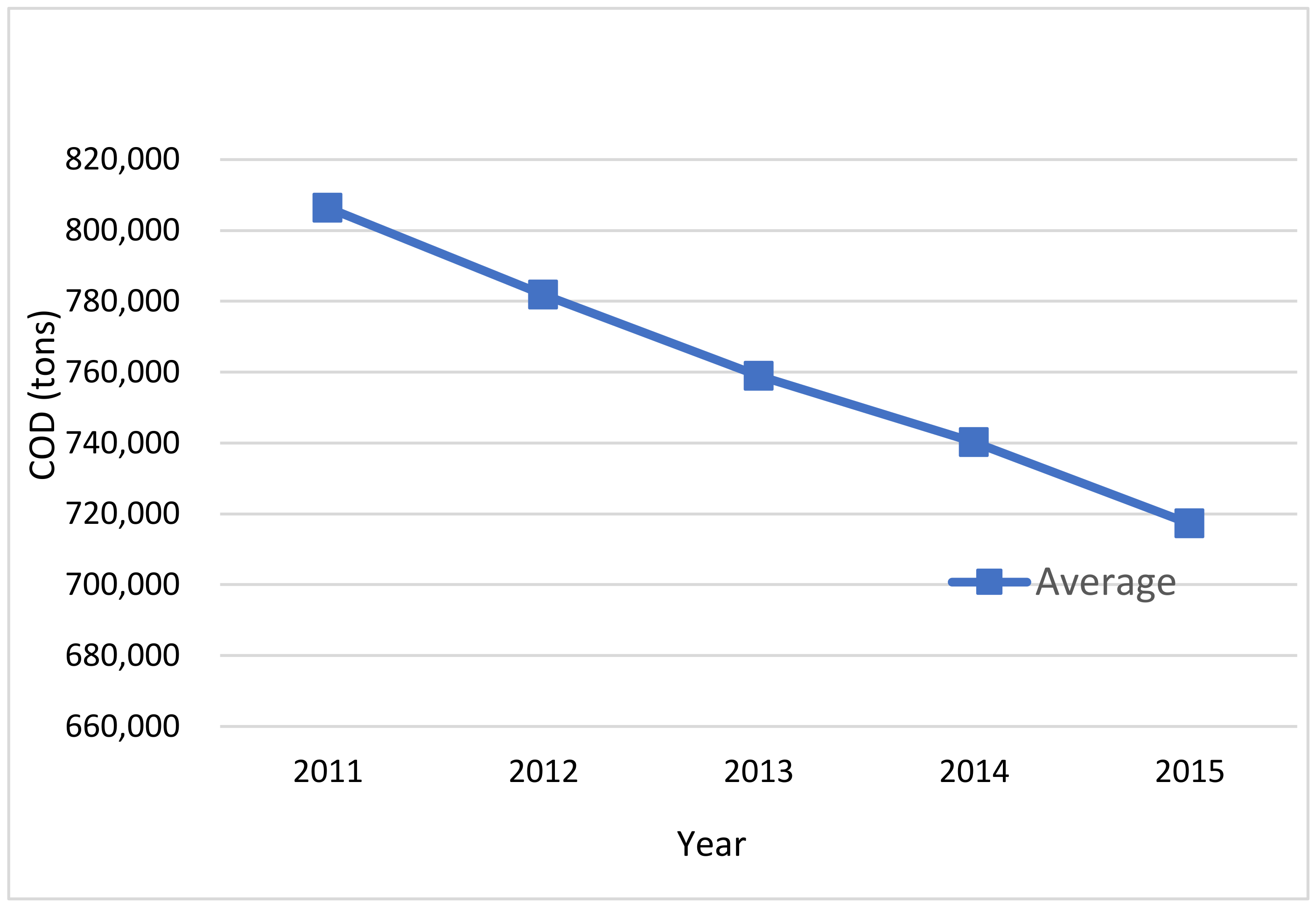
(F) COD amounts: Figure 6 shows the average COD amounts decreased by 11% from 2011 to 2015, even though total economic output rose by 38% during this period. It implies water pollution actually improved (i.e., decreased) in this period. Shandong had the most COD discharge, but it decreased from 1.982 million tons to 1.757 million tons. Tibet had the smallest discharge, but it rose from 26,800 to 28,800 tons throughout the 5 years.
3.2. Analysis of Inputs Efficiency Results from Year 2011 to 2015
Observing Table 3, we see seven regions are located on the frontier of efficiency, with a result score of 1: Beijing, Tianjin, Shanghai, Jiangsu, Zhejiang, Shandong, and Guangdong. Those regions have better economic growth, and their expense on water treatment is larger. The other four regions, Inner Mongolia, Tibet, Hainan, and Ningxia, are also efficient, characterized by small populations with less sewage, no large-scale factories, and low industrial wastewater pollution. Qinghai has a population of 57 million people, and its wastewater treatment expense is only 1/5 of the previous year at 100 million RMB. Qinghai’s discharged wastewater rose just a little by 0.1%, improving all efficiency results to 1 and allowing it to advance to the frontier in 2012.
Comparing 2012 with 2011, the overall efficiency of China regressed. Actually, the average expense on wastewater treatment was 1.11 billion RMB less than 2011. However, expense efficiencies still showed the worst results. The nine regions, which are very inefficient on wastewater pollution treatment, performed under 0.6. Gansu was the worst at 0.164, having only 1.092 billion RMB on wastewater discharge expenses. Shaanxi improved its expense efficiency to 0.680. Guangxi wastewater treatment expense was 943 (100 million), less than 1444 (100 million) in 2011.
In 2013, there were 13 regions having expense efficiencies under 0.6, making it the worst year under the 12th Five-Year Plan. These 13 regions were very inefficient on wastewater pollution treatment expenses. The drop in wastewater treatment expenses in 2012 negatively impacted on 2013’s expense efficiency. Although most regions saw better economic growth, they still neglected problems with the environment.
In 2014, Liaoning spent 242 million RMB less on wastewater treatment than in 2013. The spending in the previous year brought excellent results this year. Inner Mongolia spent 2.777 billion RMB on wastewater treatment, which is its highest yearly expense during 2011–2015, bringing it an efficiency score of 0.9906. However, its expense efficiency was only 0.0602, which is the worst over the same full period.
In 2015, there were 13 regions with expense efficiencies under 0.6. Guangxi wastewater treatment expense was 1.237 billion in 2014, more than before, resulting in an expense efficiency of 0.6251, or better than 13 regions. Six regions had expense efficiency under 0.6, which are the best results during 2011–2015. This implies the expense on wastewater discharge treatment saw lots of improvement. It was working in many regions in year 2015.
3.3. Analysis of Outputs Efficiency Results from Year 2011 to 2015
Observing Table 4, we see the wastewater efficiencies of 31 regions did not exhibit a big difference through the years 2011 to 2015. As we know, the wastewater discharged amounts increased only little. We can see overall water quality continuously improved.
3.4. Comparing Overall Efficiency Results from Year 2011 to 2015
This section compares overall efficiency during the period 2011–2015. Table 5 lists the rank and efficiency score results throughout the 5 years. Seven regions exhibited efficiency for all years. Beijing, Tianjin, Shanghai, Jiangsu, Shandong, and Guangdong are all economically developed and have stronger economic growth. These six regions have better technological facilities on discharged wastewater treatment. Another best region, Tibet, is the origin of the river in China. There are not many heavy industries and there are fewer people in this large region. Inner Mongolia, Hainan, and Ningxia are characterized by small populations, less sewage, no large-scale factories, and low industrial wastewater pollution. Hainan regressed to the worst group. Zhejiang, Fujian, Hebei, and Liaoning are developing regions with fluctuating efficiency from time to time. Chongqing began at the 27th place in the ranking and advanced to 24th, 23rd, 22nd, and 11th over the years 2011 to 2015. Shanxi, conversely, regressed from 16th to 21st, 25th, 27th, and 29th. Guangxi and Jiangxi were always the worst performing regions on wastewater discharge and economic efficiencies during the years 2011–2015.
4. Conclusions and Recommendations
Water pollution affects people’s livelihood around the world. China is a developing country with increasing urbanization and industrialization. As such, the quantity of its discharged wastewater continuously rose over the years 2011–2015, which span the 12th Five-Year Plan. As pollution accidents have taken place in recent years, it is becoming more urgent to study and improve the problem of discharged wastewater. Thus, the government should offer a sustainable development policy for the benefits of its community citizens.
4.1. Conclusions
According to the efficiency results, we see six regions are located on the efficiency frontier for all five years. Beijing, Tianjin, Shanghai, Jiangsu, Shandong, and Guangdong are economically developed regions, located close to the coast, and developed early under the economic reforms of China, thus achieving faster and more advanced economic growth. The expenses on water treatment and economic growth efficiencies in these regions are strong. Moreover, these six regions already have advanced technological facilities to handle discharged wastewater treatment.
Tibet, Inner Mongolia, Ningxia, Qinghai, and Hainan are five regions characterized by small populations with less sewage. They are not industrialized with large-scale factories. The end result is a small amount of wastewater pollution, and thus, their environment efficiency is good most of time.
Fujian, Zhejiang, Liaoning, and Jilin are the other regions close to the coast. The results showed that most of them still have good economic and wastewater discharge treatment efficiencies. Their scores placed them in the second group of efficiency. However, they still have some unstable efficiency conditions that require further understanding.
Guizhou, Gansu, Anhui, Yunnan, Guangxi, and Jiangxi mostly lagged behind. Moreover, further research is needed to help them to improve their water issues. These inland areas typically developed their economies later than the other regions. Thus, their efficiencies are not so good.
Chongqing achieved amazing score results during China’s 12th Five-Year Plan. Over the five years, it improved from 27th to then 24th, 23rd, 22nd, and 11th. Chongqing improved its efficiency score to 0.9359 in 2015. Because Chongqing continuously improved its wastewater treatment efficiency throughout the 5 years, it should be taken as a good example for other inland regions to follow. Conversely, Shanxi achieved the opposite result even after it spent more on wastewater discharge treatment from 0.354, 0.615, 0.806, 1.028, 2.382 billion RMB during the five-year period. Shanxi has the worst score results during the 12th Five-Year Plan, dropping from 16th with an efficiency score of 0.87 to 29th with an efficiency score of 0.688. Shanxi continuously fell in ranking from 16th to 21st, 25th, 27th, and 29th.
Reduced COD quantity indicates improvement in industrial wastewater discharge treatment. It was controlled for industrial pollution in 2011–2015.
The important finding of this study is that wastewater treatment expense is inefficient in many regions. For some areas, their efficiency of wastewater discharge expense is less than 60%. Instead, the efficiency of GDP and wastewater discharge is close, which do not have a big gap between them.
4.2. Recommendations
Based on the conclusions herein, we offer the following recommendations. Because economic development has moved from the coast to the inland of China, wastewater discharge issues have not been dealt with in a timely manner. According to the efficiency and rank results, the inland regions are still targeting economic development over environmental issues. It is hence necessary for the government to set up preferential or subsidy policies to encourage early water treatment projects for the inland regions. The government can formulate differentiated and workable wastewater treatment policy plans according to the development situation of a specific region. For example, Zhejiang, Fujian, Hebei, and Liaoning are regions with unstable environmental efficiency from time to time, making it necessary to further explore the causes and to adjust existing wastewater treatment methods to allow for easier improvements.
Many regions’ wastewater treatment expense efficiency is less than 60%, which implies inefficiency. It is necessary to understand the reasons for this so that the situation can be improved. Through further analysis, the government can then set an improvement policy to solve these issues under its next five-year economic plan.
A very positive note is that Chongqing continuously improved its wastewater treatment efficiency in 2011–2015. Research can be conducted to observe what Chongqing did to improve so much. This region can then be an example for others to follow. On the other hand, Shanxi regressed to the bottom rank. One-fourth of China’s coal comes from Shanxi. Therefore, a lot of coal washing water is discharged out from coal washing plants. This is a serious issue that needs to be solved urgently.
Guangxi and Jiangxi were always the worst performing regions on wastewater discharge and economic efficiency during the five-year period. Further investigation needs to be done on whether or not this is from pollution or whether it is caused by a shift to low-value industrial production.
Author Contributions
Conceptualization, Y.F. and Y.-H.C.; methodology, Y.-H.C.; software, Y.F.; validation, Y.F., Y.-H.C. and F-P.L.; formal analysis, Y.F., F-P.L.; investigation, Y.F.; resources, Y.F.; data curation, Y.F.; writing—original draft preparation, F-P.L.; writing—review and editing, F-P.L.; visualization, F-P.L.; supervision, Y.-H.C.; project administration, Y.-H.C. , F-P.L.; funding acquisition, Y.F.
Funding
This research received no external funding.
Conflicts of Interest
The authors declare no conflict of interest.
References
- Venkatesh, G.; Brattebø, H. Energy consumption, costs and environmental impacts for urban water cycle services: Case study of Oslo (Norway). Energy 2011, 36, 792–800. [Google Scholar] [CrossRef]
- Panepinto, D.; Fiore, S.; Zappone, M.; Genon, G.; Meucci, L. Evaluation of the energy efficiency of a large wastewater treatment plant in Italy. Appl. Energy 2016, 161, 404–411. [Google Scholar] [CrossRef]
- Cano, R.; Perez-Elvira, S.I.; Fdz-Polanco, F. Energy feasibility study of sludge pretreatments: A review. Appl. Energy 2015, 149, 176–185. [Google Scholar] [CrossRef]
- Panepinto, D.; Genon, G. Modeling of Po River water quality in Torino (Italy). Water Res. Manag. 2010, 24, 2937–2958. [Google Scholar] [CrossRef]
- Li, G.; Law, W.-C.; Chan, K.C. Floating, Highly Efficient, and Scalable Graphene Membranes for Seawater Desalination using Solar Energy. Green Chem. 2018, 20, 3689–3695. [Google Scholar] [CrossRef]
- Razali, M.; Kim, J.F.; Attfield, M.; Budd, P.M; Drioli, E.; Lee, Y.M.; Szekely, G. Sustainable wastewater treatment and recycling in membrane manufacturing. Green Chem. 2015, 17, 5196–5205. [Google Scholar] [CrossRef] [Green Version]
- Skouteris, G.; Ouki, S.; Foo, D.; Saroj, D.; Altini, M.; Melidis, P.; Cowley, B.; Ells, G.; Palmer, S.; O’Dell, S. Water Footprint and Water Pinch Analysis Techniques for Sustainable Water Management in the Brick-Manufacturing Industry. J. Clean. Prod. 2018, 172, 786–798. [Google Scholar] [CrossRef]
- Didaskalou, C.; Kupai, J.; Cseri, L.; Barabas, J.; Vass, E.; Holtzl, T.; Szekely, G. Membrane-Grafted Asymmetric Organocatalyst for an Integrated Synthesis-Separation Platform. ACS Catal. 2018, 8, 7430–7438. [Google Scholar] [CrossRef]
- Kumar, A.; Thakur, A.; Panesar, P.S. Acid Extraction Using Environmentally Benign Green Emulsion Ionic Liquid Membrane. J. Clean. Prod. 2018, 181, 574–583. [Google Scholar] [CrossRef]
- Liu, B.; Wang, B.; Xue, G. On assessment of public spending efficiency of environment protection in local China: Base on three-stage bootstrapped DEA. J. Zhongnan Univ. Econ. Law 2016, 1, 89–95. [Google Scholar]
- Yu, W. Government Intervention and Environmental Governance Efficiency—An Empirical Analysis Based on Provincial Panel Data. J. Yunnan Univ. Financ. Econ. 2015, 31, 132–139. [Google Scholar]
- Chen, M.; Pei, X. A Study of the Efficiency of China’s Financial Policy for Environmental Governance: Based on DEA Cross Evaluation. Contemp. Financ. Econ. 2013, 4, 27–36. [Google Scholar]
- Yang, J.; Lu, Y. Environmental Investment Efficiency in China based on three-stage DEA model. J. Syst. Eng. 2012, 27, 699–711. [Google Scholar]
- Guerrini, A.; Romano, G.; Indipendenza, A. Energy efficiency drivers in wastewater treatment plants: A double bootstrap DEA analysis. Sustainability 2017, 9, 1126. [Google Scholar] [CrossRef]
- Yang, W.; Li, L. Efficiency Evaluation and policy analysis of industrial wastewater control in China. Energies 2017, 10, 1201. [Google Scholar] [CrossRef]
- Fuentes, R.; Hernández-Sancho, F.; Torregrosa, T. Productivity of Wastewater Treatment Plants in the Valencia Autonomous Region, Spain. Int. Conf. Reg. Sci. Innov. Geogr. Spillovers New Approaches Evid. 2015, 11, 1–16. [Google Scholar]
- Castellet Viciano, L.; Molinow-Senante, M.; Hernandez-Chover, V.; Sancho, F.H. Efficiency assessment of wastewater treatment plants: A data envelopment analysis approach integrating technical, economical and environmental issues. Int. Conf. Reg. Sci. 2015, 20, 1–23. [Google Scholar] [CrossRef]
- Chiu, Y.H.; Shyu, M.K.; Lu, C.C. Undesirable output in efficiency and productivity: Example of the G20 countries. Energy Source Part B Econ. Plan. Policy 2016, 11, 237–243. [Google Scholar] [CrossRef]
- Lovell, C.A.K.; Pastor, J.T.; Turner, J.A. Measuring macroeconomic performance in the OECD: A comparison of European and non-European countries. Eur. J. Oper. Res. 1995, 87, 507–518. [Google Scholar] [CrossRef]
- Golany, B.; Roll, Y. An Application Procedure for DEA. Omega 1989, 17, 237–250. [Google Scholar] [CrossRef]
- Scheel, H. Undesirable Outputs in Efficiency Valuations. Eur. J. Oper. Res. 2001, 132, 400–410. [Google Scholar] [CrossRef]
- Hailu, A.; Veeman, T.S. Non-parametric productivity analysis with undesirable outputs: An application to the Canadian pulp and paper industry. Am. J. Agric. Econ. 2001, 83, 605–616. [Google Scholar] [CrossRef]
- Seiford, L.M.; Zhu, J. Modeling undesirable factor in efficiency evaluation. Eur. J. Oper. Res. 2002, 142, 16–20. [Google Scholar] [CrossRef]
- Seiford, L.M.; Zhu, J. A response to comments on modeling undesirable factors in efficiency evaluation. Eur. J. Oper. Res. 2005, 161, 579–581. [Google Scholar] [CrossRef]
- Chung, Y.H.; Färe, R.; Grosskopf, S. Productivity and undesirable outputs: A directional distance function approach. J. Environ. Manag. 1997, 51, 229–240. [Google Scholar] [CrossRef]
- Luenberger, D.G. Benefit functions duality. J. Math. Econ. 1992, 21, 461–481. [Google Scholar] [CrossRef]
- Shephard, R.W. Theory of Cost and Production Functions; Princeton University Press: Princeton, NJ, USA, 1970; p. 308. [Google Scholar]
- Picazo-Tadeo, A.J.; Beltrán-Esteve, M.; Gómez-Limón, J.A. Assessing eco-efficiency with directional distance functions. Eur. J. Oper. Res. 2012, 220, 798–809. [Google Scholar] [CrossRef]
- Chen, S. Energy-Save and Emission-Abate Activity with its Impact on Industrial Win-Win Development in China: 2009–2049. Econ. Rev. 2010, 3, 129–143. [Google Scholar]
- Tu, Z. The Coordination of Industrial Growth with Environment and Resource. Econ. Rev. 2008, 2, 93–105. [Google Scholar]
- Färe, R.; Grosskopf, S. Directional distance functions and slacks-based measures of efficiency. Eur. J. Oper. Res. 2010, 200, 320–322. [Google Scholar] [CrossRef]
- Chiu, C.R.; Liou, J.L.; Wu, P.I.; Fang, C.L. Decomposition of the environmental inefficiency of the meta-frontier with undesirable output. Energy Econ. 2012, 34, 19–25. [Google Scholar] [CrossRef]
- Zhang, N.; Zhou, P.; Choi, Y. Total-factor carbon emission performance of fossil fuel power plants in China: A meta-frontier non-radial Malmquist index analysis. Energy Econ. 2013, 40, 549–559. [Google Scholar] [CrossRef]
- Wang, W.; Xie, H.; Lu, F.; Zhang, X. Measuring the performance of Industrial Green Development Using a Non-Radial Directional Distance Function Approach in China. Sustainability 2017, 9, 1757. [Google Scholar] [CrossRef]
- Qin, Q.; Li, X.; Li, L.; Zhen, W.; Wei, Y. Air emissions perspective on energy efficiency: An empirical analysis of China’s coastal areas. Appl. Energy 2017, 183, 604–614. [Google Scholar] [CrossRef]
- Wang, B.; Hou, B. Empirical Study of Regional Green Development Performance in China: 1998–203—Based on Global Non-radial Directional Distance Function. J. China Univ. Geosci. 2017, 17, 24–40. [Google Scholar]
- Ben, W.; Zhu, B.; Yuan, X.; Zhang, Y.; Yang, M.; Qiang, Z. Occurrence, removal and risk of organic micro-pollutants in wastewater treatment plants across China: Comparison of wastewater treatment processes. Water Res. 2018, 130, 38–46. [Google Scholar] [CrossRef]
- Wang, Y.; Li, Y.; Hu, A.; Rashid, A.; Ashfaq, M.; Wang, Y.; Wang, H.; Luo, H.; Yu, C.P.; Sun, Q. Monitoring, mass balance and fate of pharmaceuticals and personal care products in seven wastewater treatment plants in Xiamen City, China. J. Hazard. Mater. 2018, 354, 81–90. [Google Scholar] [CrossRef]
- Färe, R.; Grosskopf, S.; Whittaker, G. Network DEA. In Modeling Data Irregularities and Structural Complexities in Data Envelopment Analysis; Zhu, J., Cook, W., Eds.; Springer: New York, NY, USA, 2007; pp. 209–240. [Google Scholar]
- Zhou, P.; Ang, B.W.; Wang, H. Energy and CO2 emission performance in electricity generation: A non-radial directional distance function approach. Eur. J. Oper. Res. 2012, 221, 625–635. [Google Scholar] [CrossRef]
- National Bureau of Statistics of China; National Bureau of Statistics Ministry of Environmental Protection. China Statistical Yearbook on Environment, 2012; China Statistics Press: Beijing, China, 2012.
- National Bureau of Statistics of China; National Bureau of Statistics Ministry of Environmental Protection. China Statistical Yearbook on Environment, 2013; China Statistics Press: Beijing, China, 2013.
- National Bureau of Statistics of China; National Bureau of Statistics Ministry of Environmental Protection. China Statistical Yearbook on Environment, 2014; China Statistics Press: Beijing, China, 2014.
- National Bureau of Statistics of China; National Bureau of Statistics Ministry of Environmental Protection. China Statistical Yearbook on Environment, 2015; China Statistics Press: Beijing, China, 2015.
- National Bureau of Statistics of China; National Bureau of Statistics Ministry of Environmental Protection. China Statistical Yearbook on Environment, 2016; China Statistics Press: Beijing, China, 2016.
Figure 1.
Average capital over 2011–2015 in China.

Figure 2.
Average population over 2011–2015 in China.
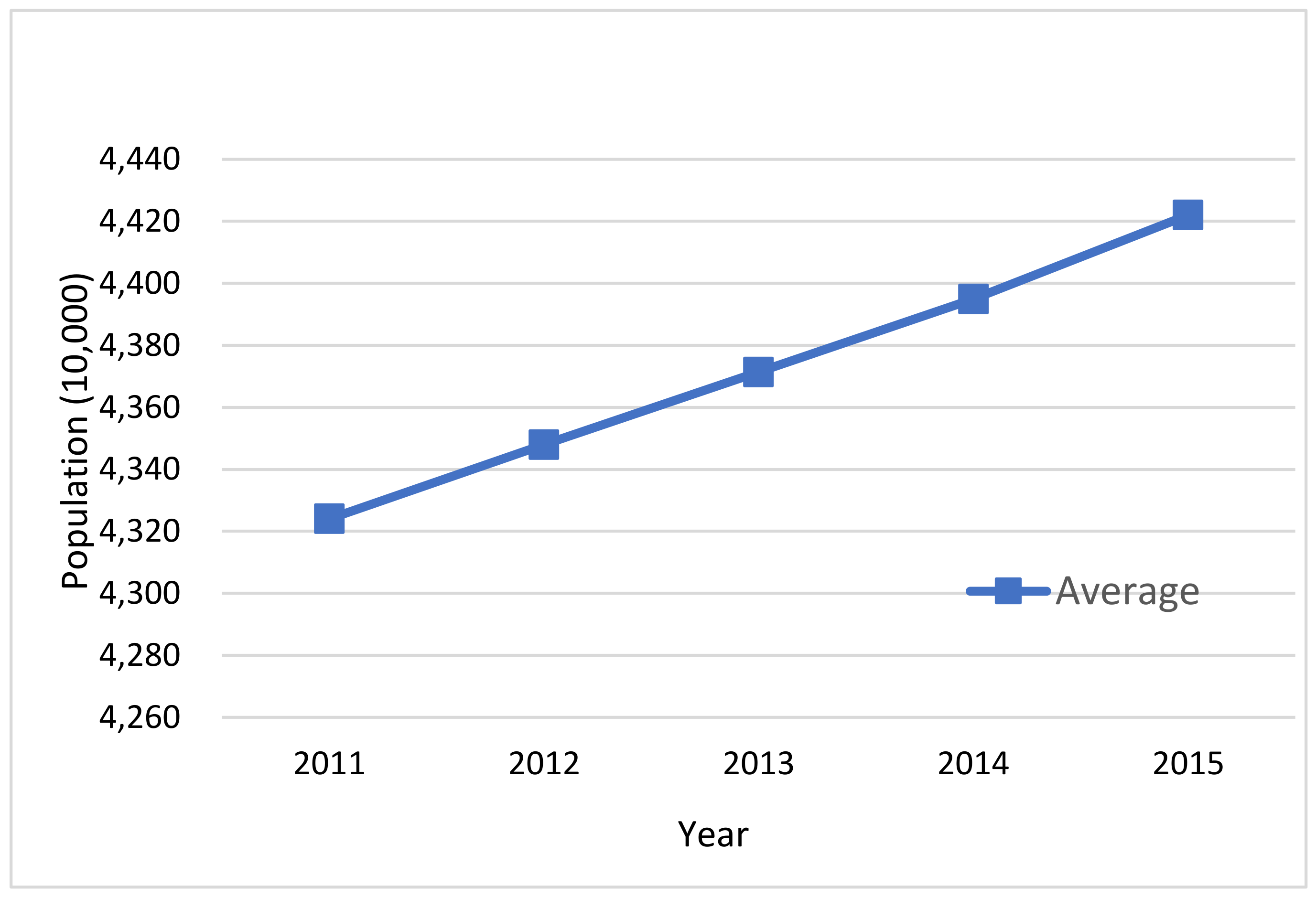
Figure 3.
Average wastewater discharge expense over 2011–2015 in China.

Figure 4.
Average GDP over 2011–2015 in China.
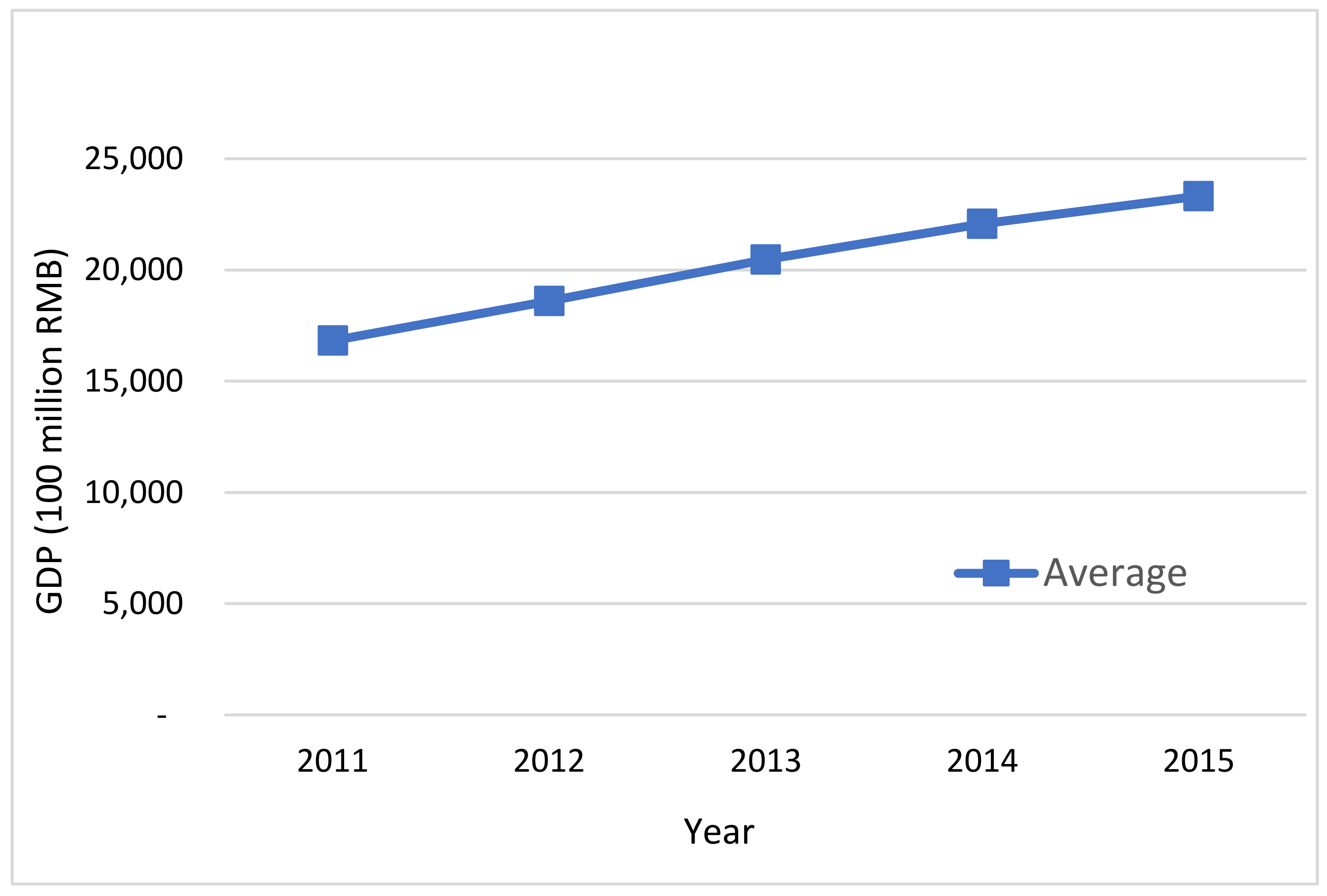
Figure 5.
Average discharged wastewater over 2011–2015 in China.
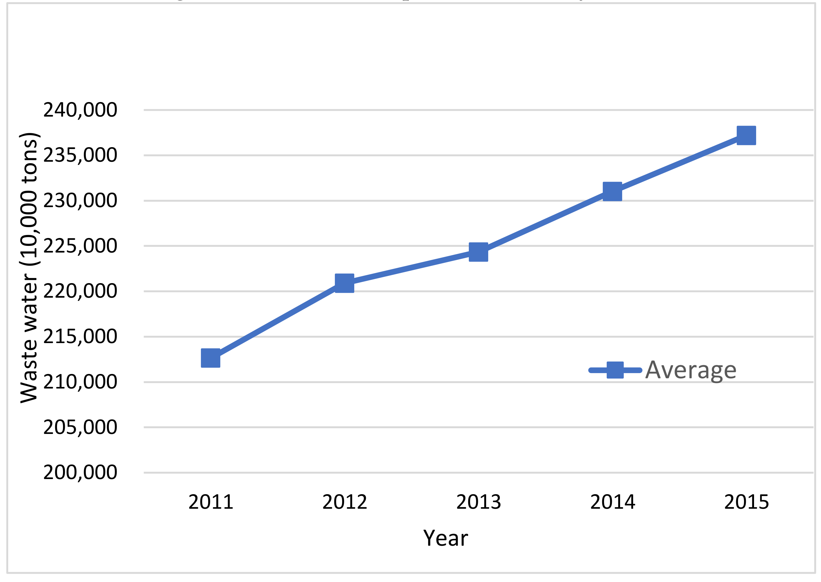
Figure 6.
Average COD over 2011–2015 in China.

Table 1.
Input and output variables. GDP: Gross domestic production, COD: Chemical oxygen demand.
| Input Variable | Output Variable |
|---|---|
| (I) Capital (I) Population (I) Expense | (O) GDP (OBad) Wastewater (OBad) COD |
Table 2.
Descriptive statistics of input–output variables.
| Year | Capital (100 Million RMB) | Population (10,000) | Expense (100 Million RMB) | GDP (100 Million RMB) | Wastewater (10,000 Tons) | COD (Tons) | |
|---|---|---|---|---|---|---|---|
| 2011 | Max | 26,749.7 | 10,505 | 58.14 | 53,210.2 | 785,587 | 1,982,497 |
| Min | 516.3 | 303 | 1.27 | 605.8 | 4635 | 26,831 | |
| Average | 9865.6 | 4324 | 12.48 | 16,820.6 | 212,643 | 806,406 | |
| SD | 6641.5 | 2769 | 11.18 | 13,216.2 | 173,996 | 534,849 | |
| 2012 | Max | 31,256.0 | 10,594 | 32.25 | 57,067.9 | 838,551 | 1,921,233 |
| Min | 670.5 | 308 | 0.06 | 701.0 | 4683 | 25,762 | |
| Average | 11,889.9 | 4348 | 11.10 | 18,598.4 | 220,891 | 781,849 | |
| SD | 7757.5 | 2778 | 8.05 | 14,325.9 | 181,034 | 514,916 | |
| 2013 | Max | 36,789.1 | 10,644 | 55.56 | 62,474.7 | 862,471 | 1,845,706 |
| Min | 876.0 | 312 | 0.59 | 815.6 | 5005 | 25,773 | |
| Average | 14,214.2 | 4371.4 | 13.97 | 20,462.6 | 224,337 | 758,942 | |
| SD | 9144.1 | 2785.7 | 12.29 | 15,709.8 | 184,430 | 496,527 | |
| 2014 | Max | 42,495.5 | 10,724 | 38.37 | 67,809.8 | 905,082 | 1,780,422 |
| Min | 1069.2 | 318 | 0.23 | 920.8 | 5450 | 27,917 | |
| Average | 16,314.6 | 4394.9 | 14.19 | 22,075.7 | 231,024 | 740,190 | |
| SD | 10,543.7 | 2797.8 | 11.17 | 16,987.7 | 190,473 | 481,404 | |
| 2015 | Max | 48,312.4 | 10,849 | 49.58 | 72,812.5 | 911,523 | 1,757,630 |
| Min | 1295.7 | 324 | 0.70 | 1026.3 | 5883 | 28,836 | |
| Average | 17,949.9 | 4422 | 15.70 | 23,315.0 | 237,200 | 717,258 | |
| SD | 11,805.4 | 2817 | 12.47 | 18,218.9 | 195,601 | 469,392 | |
| 2011 to 2015 | Change | 8084 | 98 | 3.22 | 6495 | 24,557 | −89,148 |
| Rate (%) | 82 | 2.2 | 39 | 39 | 12 | −11 | |
Table 3.
Efficiency results of inputs from 2011 to 2015.
| 2011 | 2012 | 2013 | 2014 | 2015 | ||||||
|---|---|---|---|---|---|---|---|---|---|---|
| DMU | Exp Eff * | GDP Eff * | Exp Eff * | GDP Eff * | Exp Eff * | GDP Eff * | Exp Eff * | GDP Eff * | Exp Eff * | GDP Eff * |
| Beijing | 1 | 1 | 1 | 1 | 1 | 1 | 1 | 1 | 1 | 1 |
| Tianjin | 1 | 1 | 1 | 1 | 1 | 1 | 1 | 1 | 1 | 1 |
| Inn-M * | 1 | 1 | 1 | 1 | 1 | 1 | 1 | 1 | 1 | 1 |
| Shan * | 1 | 1 | 1 | 1 | 1 | 1 | 1 | 1 | 1 | 1 |
| Jiangsu | 1 | 1 | 1 | 1 | 1 | 1 | 1 | 1 | 1 | 1 |
| Zhejia * | 1 | 1 | 1 | 1 | 1 | 1 | 1 | 1 | 1 | 1 |
| Shandong | 1 | 1 | 1 | 1 | 1 | 1 | 1 | 1 | 1 | 1 |
| Guang * | 1 | 1 | 1 | 1 | 1 | 1 | 1 | 1 | 1 | 1 |
| Tibet | 1 | 1 | 1 | 1 | 0.991 | 0.991 | 1 | 1 | 1 | 1 |
| Hainan | 1 | 1 | 1 | 1 | 0.882 | 0.960 | 0.060 | 0.990 | 0.440 | 0.978 |
| Ningxia | 1 | 1 | 0.955 | 0.957 | 0.901 | 0.910 | 0.497 | 0.940 | 0.935 | 0.939 |
| Henan | 0.996 | 0.996 | 0.624 | 0.948 | 0.723 | 0.905 | 0.136 | 0.894 | 0.930 | 0.934 |
| Xinjiang | 0.963 | 0.964 | 0.899 | 0.908 | 0.859 | 0.876 | 0.871 | 0.886 | 0.545 | 0.930 |
| Liaoning | 0.704 | 0.936 | 0.680 | 0.897 | 0.858 | 0.876 | 0.417 | 0.857 | 0.916 | 0.922 |
| Hebei | 0.525 | 0.905 | 0.752 | 0.883 | 0.837 | 0.860 | 0.832 | 0.856 | 0.896 | 0.906 |
| Shanxi | 0.870 | 0.885 | 0.849 | 0.869 | 0.825 | 0.851 | 0.784 | 0.855 | 0.831 | 0.872 |
| Shaanxi | 0.312 | 0.874 | 0.816 | 0.845 | 0.399 | 0.842 | 0.236 | 0.844 | 0.787 | 0.862 |
| Sichuan | 0.840 | 0.862 | 0.813 | 0.842 | 0.555 | 0.837 | 0.455 | 0.843 | 0.835 | 0.858 |
| Hunan | 0.652 | 0.847 | 0.811 | 0.841 | 0.280 | 0.831 | 0.385 | 0.843 | 0.585 | 0.853 |
| Heilon * | 0.557 | 0.845 | 0.493 | 0.841 | 0.478 | 0.824 | 0.187 | 0.834 | 0.821 | 0.848 |
| Jilin | 0.634 | 0.841 | 0.536 | 0.823 | 0.335 | 0.818 | 0.733 | 0.833 | 0.817 | 0.845 |
| Hubei | 0.804 | 0.836 | 0.777 | 0.817 | 0.460 | 0.802 | 0.780 | 0.819 | 0.395 | 0.828 |
| Guizhou | 0.803 | 0.835 | 0.577 | 0.813 | 0.747 | 0.798 | 0.766 | 0.810 | 0.784 | 0.822 |
| Qinghai | 0.764 | 0.827 | 0.385 | 0.808 | 0.311 | 0.795 | 0.103 | 0.797 | 0.732 | 0.788 |
| Gansu | 0.278 | 0.817 | 0.164 | 0.806 | 0.431 | 0.795 | 0.355 | 0.784 | 0.696 | 0.786 |
| Fujian | 0.517 | 0.809 | 0.520 | 0.788 | 0.263 | 0.782 | 0.465 | 0.777 | 0.710 | 0.782 |
| Chong * | 0.445 | 0.799 | 0.722 | 0.782 | 0.445 | 0.778 | 0.331 | 0.774 | 0.502 | 0.778 |
| Anhui | 0.535 | 0.780 | 0.585 | 0.777 | 0.290 | 0.775 | 0.116 | 0.765 | 0.700 | 0.769 |
| Yunnan | 0.366 | 0.763 | 0.433 | 0.755 | 0.477 | 0.758 | 0.640 | 0.763 | 0.303 | 0.762 |
| Jiangxi | 0.313 | 0.755 | 0.573 | 0.744 | 0.395 | 0.747 | 0.313 | 0.755 | 0.670 | 0.752 |
| Guangxi | 0.384 | 0.743 | 0.615 | 0.722 | 0.657 | 0.744 | 0.625 | 0.747 | 0.661 | 0.747 |
Exp Eff *: Expense efficiency, GDP Eff *: GDP efficiency; Inn-M *: Inner Mongolia, Shan *: Shanghai, Zhejia *: Zhejiang, Guang *: Guangdong, Heilon *: Heilongjiang, Chong *: Chongqing.
Table 4.
Efficiency results of outputs from 2011 to 2015.
| 2011 | 2012 | 2013 | 2014 | 2015 | ||||||
|---|---|---|---|---|---|---|---|---|---|---|
| DMU | Was Eff * | COD Eff * | Was Eff * | COD Eff * | Was Eff * | COD Eff * | Was Eff * | COD Eff * | Was Eff * | COD Eff * |
| Beijing | 1 | 1 | 1 | 1 | 1 | 1 | 1 | 1 | 1 | 1 |
| Tianjin | 1 | 1 | 1 | 1 | 1 | 1 | 1 | 1 | 1 | 1 |
| Inn-M * | 1 | 1 | 1 | 1 | 1 | 1 | 1 | 1 | 1 | 1 |
| Shan * | 1 | 1 | 1 | 1 | 1 | 1 | 1 | 1 | 1 | 1 |
| Jiangsu | 1 | 1 | 1 | 1 | 1 | 1 | 1 | 1 | 1 | 1 |
| Zhejia * | 1 | 1 | 1 | 1 | 1 | 1 | 1 | 1 | 1 | 1 |
| Shandong | 1 | 1 | 1 | 1 | 1 | 1 | 1 | 1 | 1 | 1 |
| Guang * | 1 | 1 | 1 | 1 | 1 | 1 | 1 | 1 | 1 | 1 |
| Tibet | 1 | 1 | 1 | 1 | 0.991 | 0.991 | 1 | 1 | 1 | 1 |
| Hainan | 1 | 1 | 1 | 1 | 0.959 | 0.957 | 0.990 | 0.986 | 0.977 | 0.972 |
| Ningxia | 1 | 1 | 0.955 | 0.955 | 0.901 | 0.900 | 0.936 | 0.936 | 0.935 | 0.933 |
| Henan | 0.993 | 0.993 | 0.945 | 0.943 | 0.896 | 0.882 | 0.882 | 0.881 | 0.930 | 0.929 |
| Xinjiang | 0.951 | 0.960 | 0.899 | 0.897 | 0.859 | 0.859 | 0.871 | 0.869 | 0.924 | 0.924 |
| Liaoning | 0.931 | 0.930 | 0.885 | 0.885 | 0.858 | 0.857 | 0.834 | 0.833 | 0.916 | 0.916 |
| Hebei | 0.895 | 0.895 | 0.868 | 0.867 | 0.837 | 0.834 | 0.832 | 0.831 | 0.896 | 0.896 |
| Shanxi | 0.870 | 0.868 | 0.849 | 0.848 | 0.825 | 0.823 | 0.831 | 0.830 | 0.853 | 0.851 |
| Shaanxi | 0.856 | 0.854 | 0.816 | 0.815 | 0.812 | 0.811 | 0.816 | 0.812 | 0.840 | 0.837 |
| Sichuan | 0.840 | 0.839 | 0.813 | 0.811 | 0.805 | 0.802 | 0.814 | 0.813 | 0.835 | 0.834 |
| Hunan | 0.820 | 0.818 | 0.811 | 0.809 | 0.793 | 0.796 | 0.814 | 0.812 | 0.827 | 0.824 |
| Heilon* | 0.817 | 0.813 | 0.811 | 0.808 | 0.774 | 0.783 | 0.795 | 0.799 | 0.821 | 0.819 |
| Jilin | 0.811 | 0.808 | 0.785 | 0.783 | 0.778 | 0.774 | 0.799 | 0.795 | 0.817 | 0.814 |
| Hubei | 0.804 | 0.803 | 0.777 | 0.774 | 0.753 | 0.750 | 0.780 | 0.778 | 0.793 | 0.789 |
| Guizhou | 0.803 | 0.802 | 0.770 | 0.767 | 0.747 | 0.746 | 0.766 | 0.763 | 0.784 | 0.780 |
| Qinghai | 0.790 | 0.790 | 0.763 | 0.762 | 0.743 | 0.741 | 0.745 | 0.742 | 0.732 | 0.729 |
| Gansu | 0.776 | 0.774 | 0.760 | 0.758 | 0.742 | 0.740 | 0.724 | 0.723 | 0.728 | 0.725 |
| Fujian | 0.764 | 0.763 | 0.732 | 0.729 | 0.722 | 0.720 | 0.714 | 0.711 | 0.722 | 0.719 |
| Chong * | 0.749 | 0.748 | 0.722 | 0.720 | 0.715 | 0.714 | 0.709 | 0.707 | 0.716 | 0.714 |
| Anhui | 0.718 | 0.717 | 0.713 | 0.713 | 0.709 | 0.706 | 0.693 | 0.691 | 0.700 | 0.698 |
| Yunnan | 0.690 | 0.688 | 0.676 | 0.673 | 0.682 | 0.680 | 0.690 | 0.688 | 0.688 | 0.686 |
| Jiangxi | 0.676 | 0.674 | 0.657 | 0.655 | 0.662 | 0.660 | 0.690 | 0.688 | 0.670 | 0.668 |
| Guangxi | 0.655 | 0.653 | 0.615 | 0.613 | 0.657 | 0.655 | 0.661 | 0.659 | 0.661 | 0.659 |
Was Eff *: Wastewater efficiency, COD Eff *: GDP efficiency; Inn-M *: Inner Mongolia, Shan *: Shanghai, Zhejia *: Zhejiang, Guang *: Guangdong, Heilon *: Heilongjiang, Chong *: Chongqing.
Table 5.
Rank of 31 regions in China from 2011 to 2015.
| 2011 | 2012 | 2013 | 2014 | 2015 | ||||||
|---|---|---|---|---|---|---|---|---|---|---|
| Rank | Score | Rank | Score | Rank | Score | Rank | Score | Rank | Score | |
| Beijing | 1 | 1 | 1 | 1 | 1 | 1 | 1 | 1 | 1 | 1 |
| Tianjin | 1 | 1 | 1 | 1 | 1 | 1 | 1 | 1 | 1 | 1 |
| Shanghai | 1 | 1 | 1 | 1 | 1 | 1 | 1 | 1 | 1 | 1 |
| Jiangsu | 1 | 1 | 1 | 1 | 1 | 1 | 1 | 1 | 1 | 1 |
| Shandong | 1 | 1 | 1 | 1 | 1 | 1 | 1 | 1 | 1 | 1 |
| Guangdong | 1 | 1 | 1 | 1 | 1 | 1 | 1 | 1 | 1 | 1 |
| Tibet | 1 | 1 | 1 | 1 | 1 | 1 | 1 | 1 | 1 | 1 |
| Inner Mongolia | 1 | 1 | 1 | 1 | 1 | 1 | 10 | 0.990 | 10 | 0.977 |
| Ningxia | 1 | 1 | 1 | 1 | 20 | 0.797 | 1 | 1 | 1 | 1 |
| Zhejiang | 1 | 1 | 11 | 0.955 | 9 | 0.991 | 11 | 0.936 | 13 | 0.924 |
| Hainan | 1 | 1 | 22 | 0.777 | 22 | 0.753 | 23 | 0.766 | 12 | 0.93 |
| Henan | 12 | 0.996 | 16 | 0.849 | 13 | 0.859 | 15 | 0.832 | 18 | 0.835 |
| Xinjiang | 13 | 0.963 | 26 | 0.732 | 28 | 0.709 | 26 | 0.714 | 24 | 0.732 |
| Liaoning | 14 | 0.932 | 12 | 0.945 | 10 | 0.959 | 1 | 1 | 1 | 1 |
| Hebei | 15 | 0.896 | 15 | 0.868 | 11 | 0.901 | 13 | 0.871 | 15 | 0.896 |
| Shanxi | 16 | 0.87 | 21 | 0.785 | 25 | 0.742 | 27 | 0.709 | 29 | 0.688 |
| Shaanxi | 17 | 0.856 | 14 | 0.885 | 12 | 0.896 | 12 | 0.882 | 21 | 0.817 |
| Sichuan | 18 | 0.841 | 13 | 0.899 | 14 | 0.858 | 19 | 0.814 | 20 | 0.821 |
| Hunan | 19 | 0.821 | 19 | 0.811 | 18 | 0.805 | 18 | 0.815 | 19 | 0.827 |
| Heilongjiang | 20 | 0.817 | 23 | 0.770 | 21 | 0.778 | 21 | 0.799 | 23 | 0.784 |
| Jilin | 21 | 0.811 | 20 | 0.811 | 15 | 0.837 | 17 | 0.816 | 22 | 0.793 |
| Hubei | 22 | 0.804 | 18 | 0.813 | 17 | 0.812 | 16 | 0.831 | 17 | 0.840 |
| Guizhou | 23 | 0.803 | 27 | 0.722 | 26 | 0.722 | 28 | 0.693 | 27 | 0.716 |
| Qinghai | 24 | 0.791 | 28 | 0.713 | 19 | 0.797 | 20 | 0.801 | 14 | 0.916 |
| Gansu | 25 | 0.777 | 25 | 0.760 | 24 | 0.743 | 24 | 0.745 | 25 | 0.728 |
| Fujian | 26 | 0.764 | 17 | 0.816 | 16 | 0.825 | 14 | 0.834 | 16 | 0.853 |
| Chongqing | 27 | 0.749 | 24 | 0.763 | 23 | 0.747 | 22 | 0.780 | 11 | 0.935 |
| Anhui | 28 | 0.718 | 28 | 0.713 | 27 | 0.715 | 25 | 0.724 | 26 | 0.722 |
| Yunnan | 29 | 0.691 | 29 | 0.676 | 29 | 0.682 | 29 | 0.690 | 28 | 0.700 |
| Guangxi | 30 | 0.677 | 31 | 0.615 | 31 | 0.657 | 31 | 0.661 | 30 | 0.670 |
| Jiangxi | 31 | 0.656 | 30 | 0.657 | 30 | 0.662 | 30 | 0.68 | 31 | 0.661 |
© 2019 by the authors. Licensee MDPI, Basel, Switzerland. This article is an open access article distributed under the terms and conditions of the Creative Commons Attribution (CC BY) license (http://creativecommons.org/licenses/by/4.0/).
Share and Cite
MDPI and ACS Style
Feng, Y.; Chiu, Y.-h.; Liu, F.-p. Measuring the Performance of Wastewater Treatment in China. Appl. Sci. 2019, 9, 153. https://doi.org/10.3390/app9010153
AMA Style
Feng Y, Chiu Y-h, Liu F-p. Measuring the Performance of Wastewater Treatment in China. Applied Sciences. 2019; 9(1):153. https://doi.org/10.3390/app9010153
Chicago/Turabian StyleFeng, Ying, Yung-ho Chiu, and Fan-peng Liu. 2019. "Measuring the Performance of Wastewater Treatment in China" Applied Sciences 9, no. 1: 153. https://doi.org/10.3390/app9010153
Note that from the first issue of 2016, this journal uses article numbers instead of page numbers. See further details here.