Use of Fiber-Optic Sensors for the Detection of the Rail Vehicles and Monitoring of the Rock Mass Dynamic Response Due to Railway Rolling Stock for the Civil Engineering Needs

Abstract

The paper describes the original results of a comparative study of the standard seismic station vs. a novel interferometric sensor for civil engineering needs. The presented results showed that to implement seismic measurements using standard seismic stations, a method using a fiber optic interferometer may serve as an alternative. We presented time records and the frequency spectra obtained from experimental measurements of the dynamic response of the upper rock mass beneath passing tram vehicles (a total of 769 passes) over a period of five months of practical measurements under various climatic conditions. The fiber-optic sensor detected all phenomena at a 100% rate, and the recorded results were compared to the results from a standard seismic station. Both sets of results were recorded simultaneously and agreed significantly, especially in terms of frequency. With regard to time, all tram vehicle axles were detected in individual time records. With regard to frequency, the results detected in the bandwidth generally correlated to rail transport for individual types of tram vehicles.

1. Introduction

As a tram travels, sets of vibrations occur, which are transmitted to the bedrock. The intensity of these vibrations depends on the type and age of trams in operation, the structure and condition of the roadbed, the local geological composition, and distance from the railway yard. Vibrations formed in this way can have an adverse effect on the surrounding structures, people living near these structures, and on the technologies situated in them. Experimental measurements are therefore necessary in order to obtain data that represent such vibrations. To implement seismic measurements using standard seismic stations, a method using a fiber optic interferometer may serve as an alternative.

Fiber-optic interferometers (such as Mach–Zehnder, Sagnac, Michelson, or Fabry–Perot) are well known for their ability to make high-precision measurements of optical path differences or changes induced by a refractive index change in the interferometer or physical displacement [1]. The inherent advantages of fiber-optic interferometers are their small size, electrical passivity, immunity to electromagnetic interference (EMI), and low attenuation (which allows the measuring point to be separated from the point of evaluation).

Electrical and electromagnetic sensors currently used to monitor rail transport have problems with reliability in their function. A primary reason for this reduced reliability is the new traction drives of rail vehicles, which generate electromagnetic interference and signal contamination caused by the traction return current in rails. Another problem with electrical detection systems is low resistance to the effect of or damage from atmospheric discharge. In devices with metallic connections, undesirable conductive loops are closed over these electrically-conductive circuits, which are very hard to treat [2,3].

By using the proposed fiber-optic interferometric sensor, which is designed with regard to materials characterized by EMI, these problems can be eliminated. This article focuses, except the innovative detection of passing tram rail vehicles, on the partial comparison of the original data obtained during experimental measurements of the dynamic response of the rock mass beneath the railway rolling stock using both mentioned methods. Monitoring the effect of vibrations, i.e., maximum amplitudes and frequencies, is highly important due to their effect both on building structures and humans. Vibrations from the source are spread via the rock mass and attenuated depending on increasing distance. Vibrations in near-surface sediments can be strengthened; resonant vibrations are caused in the near-surface layer, and the duration of vibrations is prolonged because of freely-vibrating near-surface sediments. Frequencies themselves then play a highly important role in potential structural damage to buildings, especially if the resonance of an object’s frequency and the frequency of the load source is achieved. The long-term effect of vibrations on buildings may include the formation of cracks in plaster and masonry or other defects.

The scope of the maximum amplitudes and frequencies of measured values are defined for railway transport in ISO 4866:2010 [4]:

• maximum range of shifts: 1–200 $\mathsf{\mu }$m,
• maximum range of vibration speed amplitude: 0.2–50 mm·s${}^{-1}$,
• maximum range of acceleration amplitude: 0.02–1 m·s${}^{-2}$,
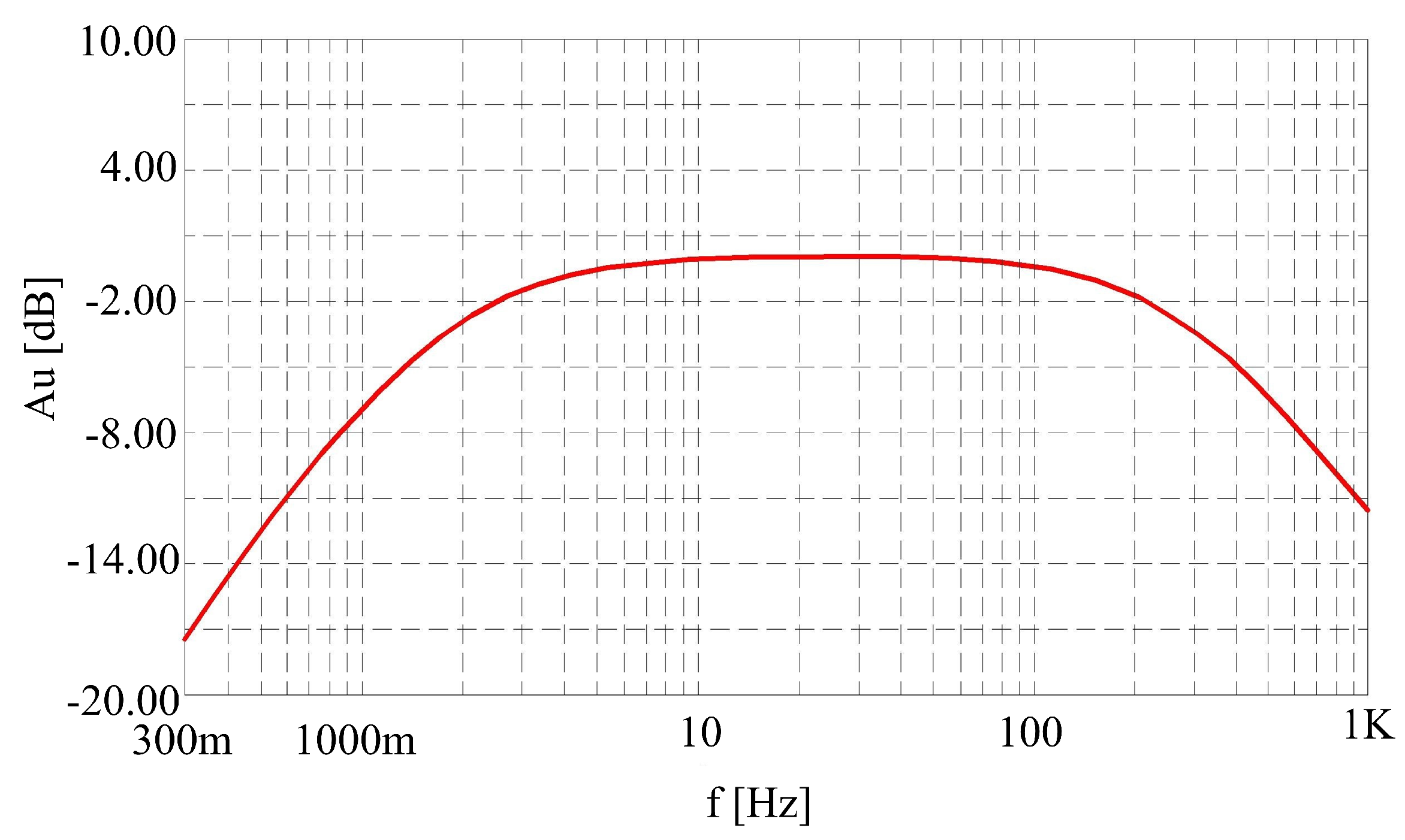
• frequency range: 1–80 Hz.

Seismic stations [5,6,7] made by recognized companies come equipped with speed and acceleration sensors and are commonly used to measure the effect of vibrations or to detect rail vehicles. Time records are generated showing the passing of a vehicle. Frequency spectra are subsequently calculated in the relevant software. The cost of these devices is often in the thousands of U.S. dollars [8,9,10]. This study used a Gaia 2T apparatus with ViGeo2 seismic sensor station as a reference seismic station to an interferometric sensor. The present paper shows that an optical interferometric sensor is a suitable alternative to a seismic station and has a price lower by an order of magnitude (for the details, please see the Discussion).

One of the basic tasks of seismic engineering in measuring the dynamic effects of ground vibrations is determining the dynamic response and attenuation parameters of the rock mass environment. For this purpose, seismic measurements are performed directly in the terrain. In order to verify the possibility of using an optical interferometer for similar purposes, this measurement was carried out in the field on a known rock mass. For the experiment, we chose such a place where there were no other disturbing sources like traffic (the nearest road was closed) or other human activities.

The monitored parameters described in this paper are sets of generated frequencies caused by passing light rail vehicles. Time records characterizing the detection of individual vehicles are dealt with in detail. Construction of the interferometric sensor is also described in detail, and the software application for data evaluation is explained (detection of vehicles and evaluation of frequency spectra).

Table 1. A comparison of the basic parameters of the proposed interferometric sensor and used seismic station.

Type of Sensor	Frequency Range (Hz)	Sampling Frequency (Hz)	Recording	Size (mm)	Weight (kg)	Price in Dollars
Gaia 2T + ViGeo2	2–200	20–500	Switch on and continual	280 × 240 × 130 + 130 × 110	4 + 2.75	2500 and more
Interferometric sensor	2–100	1000–10,000	Switch on and continual	500 × 500 × 130	3	500

shows a comparison of the basic parameters of the proposed interferometric sensor and used seismic station.

2. State-of-the-Art

The authors of [11] provided interesting results describing bridge statics and a dynamic vibration monitoring system. In that study, two different types of cameras were used to monitor the response of a bridge to a passing train. The acquired images were analyzed using three different image processing techniques (pattern matching, edge detection, and digital image correlation), and the results were compared to reference measurements obtained by a laser interferometer providing single point measurements. The authors of [12] made use of an in-fiber Fabry–Perot interferometer with fiber Bragg grating mirrors (FBG-FPI). The authors suggested that this type of sensor could be used to monitor a wide range of vibration frequencies. One of the possible applications is in monitoring seismic responses. The work in [13] compared and assessed the suitability of two methods of geodetic measurements (interferometric measurement and tachymetry measurement). The tachymetry measurements were conducted using a Leica TC2002. An IBIS microwave coherent radar was used for the interferometry method. The authors monitored dynamic changes caused by passing trains. The experimental results could be used to determine the changes in the geometric condition of buildings and engineering structures. The authors of [14,15,16] focused on the use of a fiber-optic interferometer in motor vehicle traffic or for perimetric applications. A sensor on the Mach–Zehnder interferometer was constructed to detect vibration and acoustic responses caused by humans and vehicles moving around the sensor. The authors described the possible use of this sensor to monitor traffic density, vibrations from roadways, and noise in cities dynamically. Another publication described a strain meter based on a laser interferometer. This sensor provided a new method for observing low-frequency ground motion on seismic, geodetic, and intermediate timescales, as described by the authors of [17]. A study of the geophysical response of fiber-optic acoustic sensors in laboratory-scale experiments was described in [18]. The authors analyzed acoustic data recorded simultaneously by a fiber-optic interferometer (Michelson type) and conventional three-component accelerometers.

Another use of interferometric sensors was described in [19,20]. The authors of [19] reflected on the use of an acoustic fiber-optic sensor to monitor railway infrastructure from a long distance on the basis of an interferometric connection. The work in [20] described the implementation of optical sensors with a Fabry–Perot interferometer during the production of pre-stressed, pre-fabricated concrete, and steel sleepers. These sensors can be used to calculate the number of axles, as well as the direction and speed of a train with additional sensors. In the patent described in [21], an interferometric sensor was used to detect railway vehicles and calculate their number of axles, i.e., an axle counter. The principle of detection used in this patent is based on scanning vibration responses as trains pass. To apply this sensor, its sensing element must be placed in direct physical contact with the rails. The reference element, including its evaluation component, is then placed away from the rails. In patent [22], the basic principle of a railway vehicle axle counter based on a fiber-optic interferometer is described. The sensing element of the optical fiber of the interferometer is physically attached to the rail, and a multimode optical fiber is included in the railhead. A change in the geometry of the optical fiber because of the pressure exerted on the fiber by a passing railway vehicle changes the speckle images of the measuring fiber. The work in [23] described the use of a Mach–Zehnder fiber-optic interferometer to monitor car traffic, for detecting vehicles, and measuring their speed. A Mach–Zehnder interferometer for rail transport was described in [24], which analyzed the use of a three-armed Mach–Zehnder interferometer in rail traffic as a traffic density detector.

Seismic devices are commonly used for a wide range of applications. In geotechnical engineering, they are most commonly used for in situ measurements of vibrations, monitoring during blasting operations at mines, or during underground construction employing blasting or heavy vibration demolition techniques (e.g., hydraulic hammers) to monitor the dynamic response of buildings or rock mass [25,26,27,28]. In urban areas, the dynamic effect of traffic on buildings and their surroundings has been monitored [29,30,31,32,33,34]. Another branch of seismic engineering where these stations are often used is in the determination of natural seismicity for micro-seismic rationing and operational use in service measurements of induced seismicity (e.g., [34]). Our aim was that the presented solution and information could be used for future research in civil engineering, especially in monitoring the condition of buildings and their possible susceptibility to damage caused by rolling stock.

However, no publication is available for civil engineering needs. Our publication brings original results of a comparative study of the interferometric sensor and the standard seismic station equipped with a three-component high-speed seismometer.

3. Methods

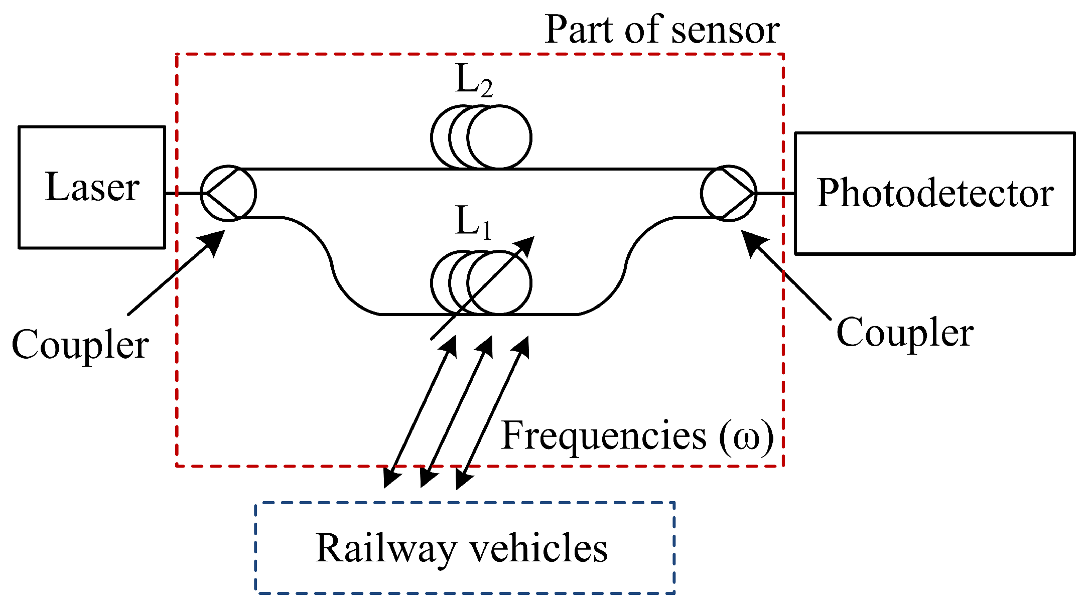
3.1. Fiber-Optic Interferometry and Signal Processing

Light interference in optical fibers was selected as an underlying phenomenon because it is highly sensitive and allows frequency changes from several Hz to several kHz to be monitored. Figure 1 shows a simplified scheme of the interferometric sensor used based on the two-armed Mach–Zehnder interferometer. A passing railway vehicle near a sensor (Figure 1) causes a response ($\omega$) with low frequencies in the range of several Hz up to hundreds of Hz [35,36,37]. This vibration and acoustic response excite the measurement fiber of the interferometric sensor and cause a change in its optical length, or more precisely, the product of its refractive index nand geometric length L. The resulting phase change $\Delta \varphi$ is given by the phase changes of the light source ($\Delta {\varphi }_1$) and the changes in the length of the arm and its refractive index ($\Delta {\varphi }_2$). The phase changes of the source ($\Delta {\varphi }_1$) occur in both arms of the interferometric sensor (reference $L_2$ and measurement $L_1$ arms), and one is subtracted from the other, while the phase changes due to a vibration source ($\Delta {\varphi }_2$) that contain information about measured frequencies ($\omega$) caused by a passing railway vehicle only occur in the measurement arm of the interferometric sensor.

In the presented solution, the evaluation unit consists of several parts: a laser (MCLS1 Thorlabs, wavelength 1550 nm) with a reference power of 1 mW; a photodetector (Thorlabs PDA10CS-EC, InGaAs 700–1800 nm); an analogue-digital (A/D) converter, used as a measuring card (NI USB 6210 National Instruments, Austin, TX, USA); an analogue first-order high-pass (HP) filter with a corner frequency of 2 Hz; and a computer (PC). The presented solution (sensor and evaluation unit) was based on conventional single-mode G.652 optical fibers. A simplified block diagram of the sensor system’s detection component is shown in Figure 2.

Optical signals from the reference ($L_2$) and the sensing ($L_1$) arms of the interferometric sensor merge with a coupling ratio of 2:1 in the optical coupler (SMF-28E, 9/125 $\mathsf{\mu }$m fiber, 3.0-mm jacket protection, length of individual arms 1.5 m), whose output is connected to a photodetector (PD). The resulting intensity of optical radiation falling on the photodetector is sufficient for the phase change between the light beams scattered through the interferometer arms. The output of the photodetector is a voltage signal (with sufficient overall power for collected light, i.e., the phase), which can be described as the sum of two signals:

$$u\left(t\right)=p\left(t\right)+e\left(t\right),$$

(1)

where $p\left(t\right)$ is the desired signal (vibration and acoustic response) detected by the interferometric sensor and $e\left(t\right)$ is the error signal caused by the instability of light polarization and external influences (temperature). The error signal can be described as a slow change in phase with a frequency that is one order of magnitude less than the lowest frequency of the desired signal $p\left(t\right)$. Because of this difference, the first-order high-pass (HP) filter mentioned above with a corner frequency of 2 Hz can be used to separate $e\left(t\right)$ from $p\left(t\right)$. The use of an analogue filter before the A/D converter with the stated parameters seems to be optimal, as it improves the dynamic range of measurement and practically leads to removal of the DC component and low frequency components (signal $e\left(t\right)$ from the measured signal $p\left(t\right)$.)

The output intensity of the interferometer is expressed by the following equation:

$$I=2I_0\left\{1+cos\left[\frac{2\pi }{\lambda }n\left(L_1-L_2\right)\right]\right\},$$

(2)

where $L_1$ and $L_2$ indicate the length of the measurement and reference arms of the interferometer, $I_0$ is the medium signal value, and $\lambda$ is the wavelength of the radiation source. The intensity of the interferometer output is converted to an electric current by means of an optical receiver (a photodetector):

$$i=\epsilon I_0\alpha cos\left({\varphi }_d+{\varphi }_{s}sin\omega t\right),$$

(3)

where $\epsilon$ is the sensitivity of the photodetector, $\alpha$ represents the losses on the interferometer, $I_0$ is the medium signal value, ${\varphi }_d$ is the changing phase shift, ${\varphi }_s$ is the duration of the amplitude, and $\omega$ symbolizes the frequencies applied to the sensing arm of the interferometer [38,39,40,41,42].

The monitoring application (PC) for vehicle detection and frequency analysis measurement was developed in LabVIEW (2015, National Instruments, Austin, TX, USA). The sampling frequency was set to 1 kHz (this value is sufficient with regards to the measured range of 1–80 Hz stated in ISO 4866:1990 for rail transport). Measurement of the vibration spectrum (generated by a tram) is triggered by the tram detection algorithm. The algorithm (for the interferometric sensor) evaluates the overall RMS value of vibrations generated by a passing tram. The algorithm searches for the first amplitude spike (caused by the first axle of the passing tram) over the set level (minimum 3 dB), which is determined with respect to the measured background noise of the interferometric sensor.

To improve the sensor’s tolerance (immunity) of external influences (noise) occurring in the vicinity of the sensor, each segment of the measured data was converted from an absolute value to a relative level $L_{noise}$, which relates to background noise as follows:

$$L_{noise}=10log\left(\frac{P_{noise}}{P_0}\right),$$

(4)

where $P_{noise}$ is the current RMS value calculated from the signal segment on the filter’s output and $P_0$ is the average RMS noise value. The value of $P_0$ was calculated as a moving average (MA) over period T according to:

$$P_0=\frac{{\sum }_{t=0}^T\sqrt{\frac{1}{N}{\sum }_{i=0}^{N-1}x{\left[n\right]}^2}}{T},$$

(5)

where $x\left[n\right]$ are individual samples in the data window with a size of N. The duration of the data segment in which the calculations were performed depended on the number of samples acquired for the calculation of the $P_{noise}$ RMS value. The default duration was 100 ms, with the algorithm showing more immunity to noise for larger data segments, however with a less accurate detection of the passage of time and an overall reduction in sensitivity.

Once a passing tram is detected, the application begins recording the signal samples $x_n$ from the interferometer. The length of recording $N_{REC}$ is a fixed pre-set value, usually several seconds. The recorded signal is then used to calculate the frequency spectrum $X_k$, where:

$$X_k=\sum _{n=0}^{N_{REC}-1}{x}_n\left(cos\left(-2\pi k\frac{n}{N_{REC}}\right)+jsin\left(-2\pi k\frac{n}{N_{REC}}\right)\right),k\in Z.$$

(6)

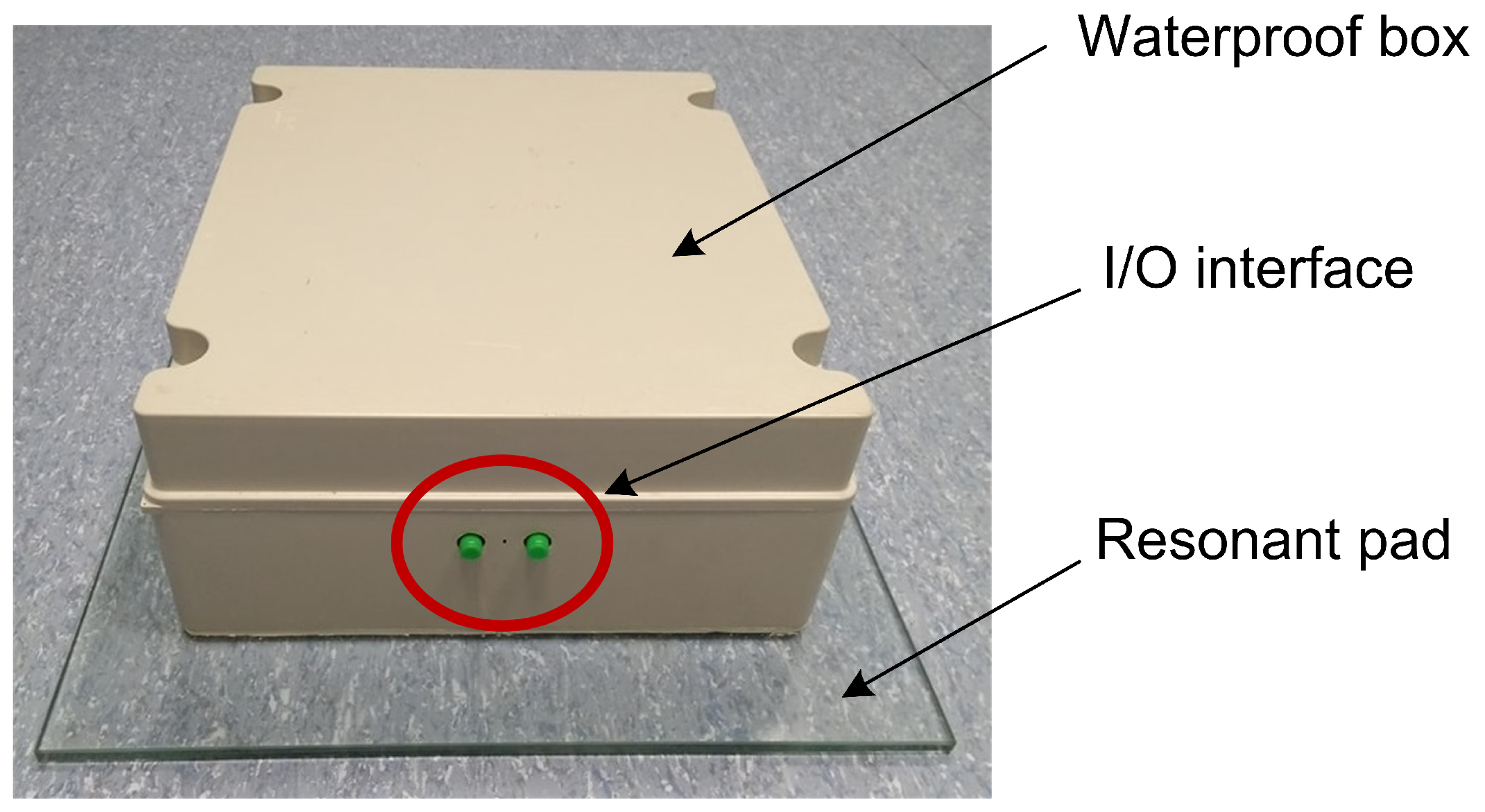
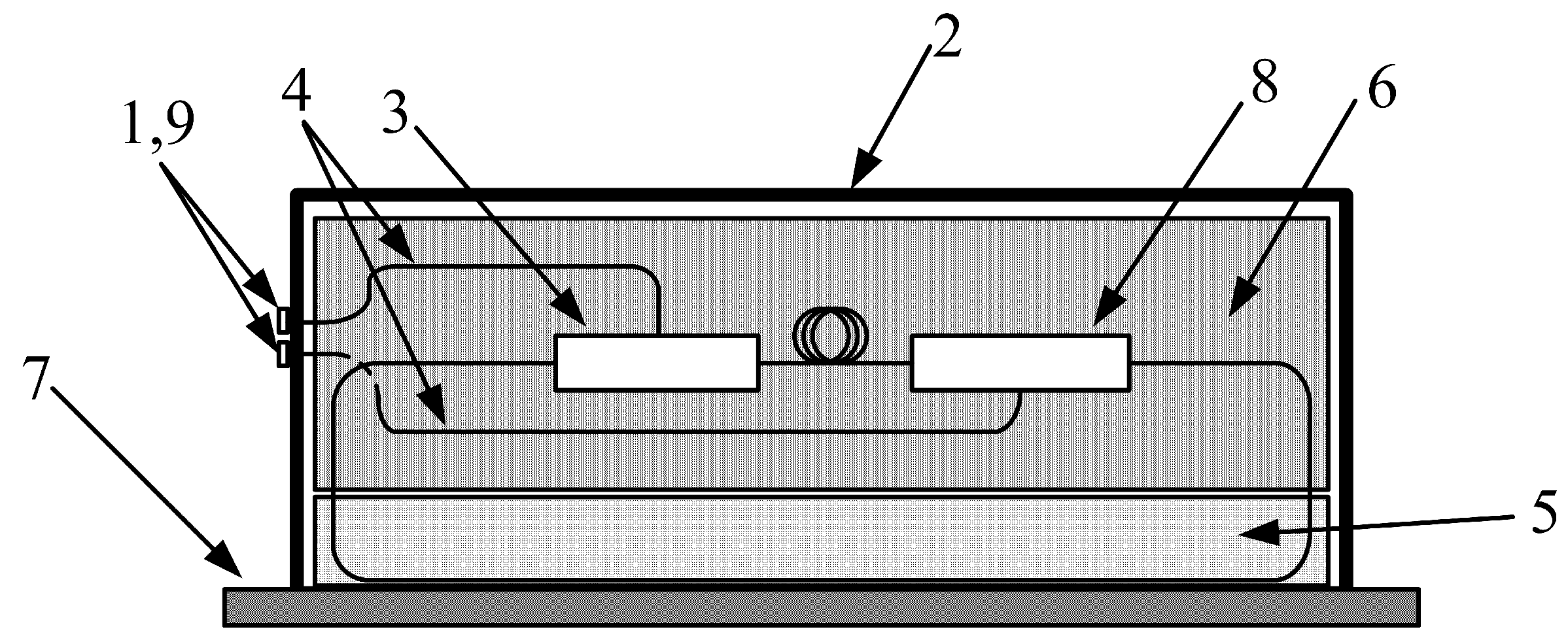
3.2. Interferometric Sensor Unit

The process of constructing the measurement sensor can be divided into several steps. The main step in designing the interferometer sensor is correct positioning of its reference ($L_2$) arm and selecting the so-called “resonant pad” on which to place the measurement ($L_1$) arm. The reference arm material should be able to dampen any external influences applied to the reference optical fiber sufficiently. The measurement arm material should be of adequate quality to support attachment of this part of the sensor. In brief, the resonant pad needs to be placed on an elevated part of the trackside, and it should be able to transmit a vibration response from the surface to the measurement optical fiber ($L_1$). It should also allow the interferometer to be placed in a box that is resistant to external conditions. The dimensions of the waterproof plastic protective box were 40 × 30 × 12 cm (height, width, depth). It should also facilitate an I/O interface suitable for direct connection to feed single-mode telecommunications optical fibers (G.652).

For the final construction of the damped part of the sensor, polystyrene foam was chosen because of its low thermal conductivity and ability to dampen higher frequencies. The tested minimum value for sufficient dampening of vibration transmission to the optical fiber was determined as 5 cm, mainly because of the sensitivity and frequency range of the interferometric sensor. Further, we tested the methodologies of installing measurement and reference fibers, waterproof boxes, splitters, fastening and housing materials, and optical fiber protections; please see our publications [43,44,45,46,47].

For the final construction of the resonant pad of the sensor, we chose glass (soda-lime glass) as an ideal material to contain the interferometer’s measuring fiber. A series of laboratory measurements were carried out to verify the effect of the thickness and size of the glass (resonant pad) on the transmission of vibrations to the measuring ($L_1$) optical fiber. A thickness of 1 cm and a size of 50 × 50 cm was selected (please see the publication [45]); these values showed a compromise with regard to sensitivity, frequency range, price, and practical installation. A photo of the fiber-optic interferometric sensor prototype is shown in Figure 3. The I/O interface of the sensor consists of the FC/APCconnectors (labeled red in Figure 3).

Figure 4 below shows a longitudinal section of the sensory unit prototype.

The symbols in Figure 4 indicate:

• Input/output interfaces (FC/APC connectors).
• Protective plastic waterproof box.
• Optical Coupler No. 1.
• Conventional G.652 optical fiber.
• Location of the measuring ($L_1$) arm of the interferometer.
• Location of the reference ($L_2$) arm of the interferometer.
• Resonant pad.
• Optical Coupler No. 2.
• Input/output interfaces (FC/APC connectors).

The measuring arm is fixed directly (along with its entire length on the resonant pad). The dark grey part shows a part of the sensor, where a reference arm and both couplers are stored in the used polystyrene foam. The light grey part of the sensor shows a part of the storing of a measuring arm. The distance between the resonant pad with the fixed measuring arm and the dark grey part is 5 cm.

Figure 5 shows the analyzed frequency characteristic of the interferometric sensor. The highest sensitivity was achieved in the range 2–100 Hz. Sensitivity levels in the range 2–100 Hz (in accordance with ISO 4866:1990, which states the range for rail transport as 1–80 Hz) were achieved by the design arrangement of the sensor described above.

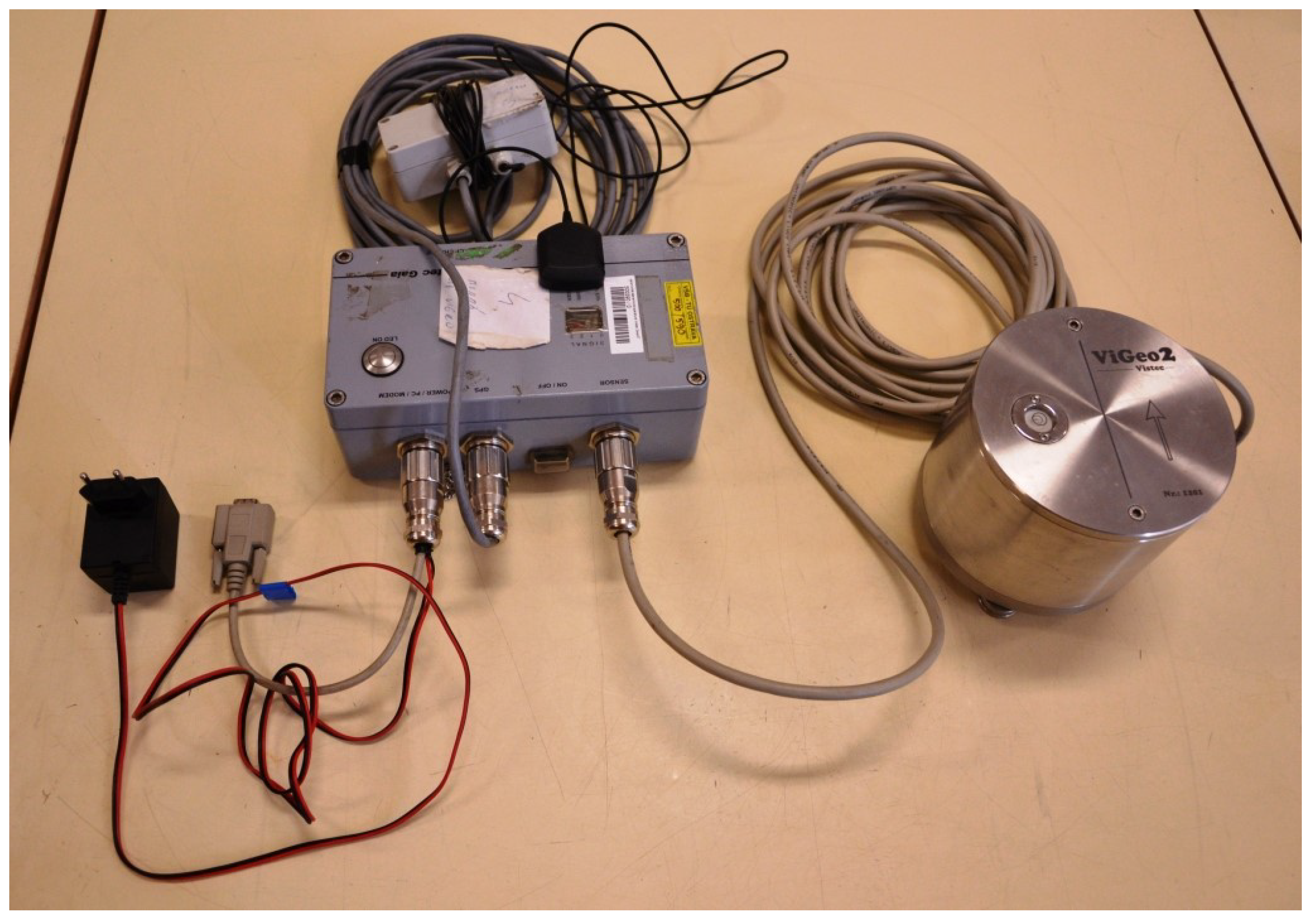
3.3. Seismic Equipment Gaia 2T

As reference equipment, a Gaia 2T apparatus with ViGeo2 seismic sensors was used (made by Vistec, Praha). The Gaia 2T equipment is a three-channel seismic station with a dynamic range of 138 dBp-ps and the option for triggered or continuous digital data recording. Synchronization of time was provided with a GPS module, and data were recorded on compact flash drives. ViGeo2 is a compact, active, short-period, three-component, high-speed seismometer for field and stationary applications. The seismometer includes three mechanical vibrating systems (sensors) with a frequency of 2 Hz and a frequency range of 2–200 Hz. The frequency range of the sensor is shown in Figure 6; the horizontal axis shows frequency, and the vertical shows amplitude.

Figure 7 shows the complete assembly of a standard Gaia 2T seismic station with the ViGeo2 speed sensor made by Vistec. It includes a GPS antenna for synchronizing time and a data and power supply cable.

The SWIP program (Seismic Waves Interpretation Program) delivered as the standard by Vistec Praha to Gaia Instruments was used to process seismic data. This program enables a seismic signal to be processed according to both time and frequency. In regard to amplitude, the processing software does not allow the values of vibration amplitudes to be recalculated into physical units (mm·s${}^{-1}$); therefore, the vertical axes in all figures showing wave images are plotted in quantization levels (cnt). The conversion formula for the ViGeo2 sensor is as follows: $1cnt=2.975\times {10}^{-6}$ mm·s${}^{-1}$ (more in [48,49])

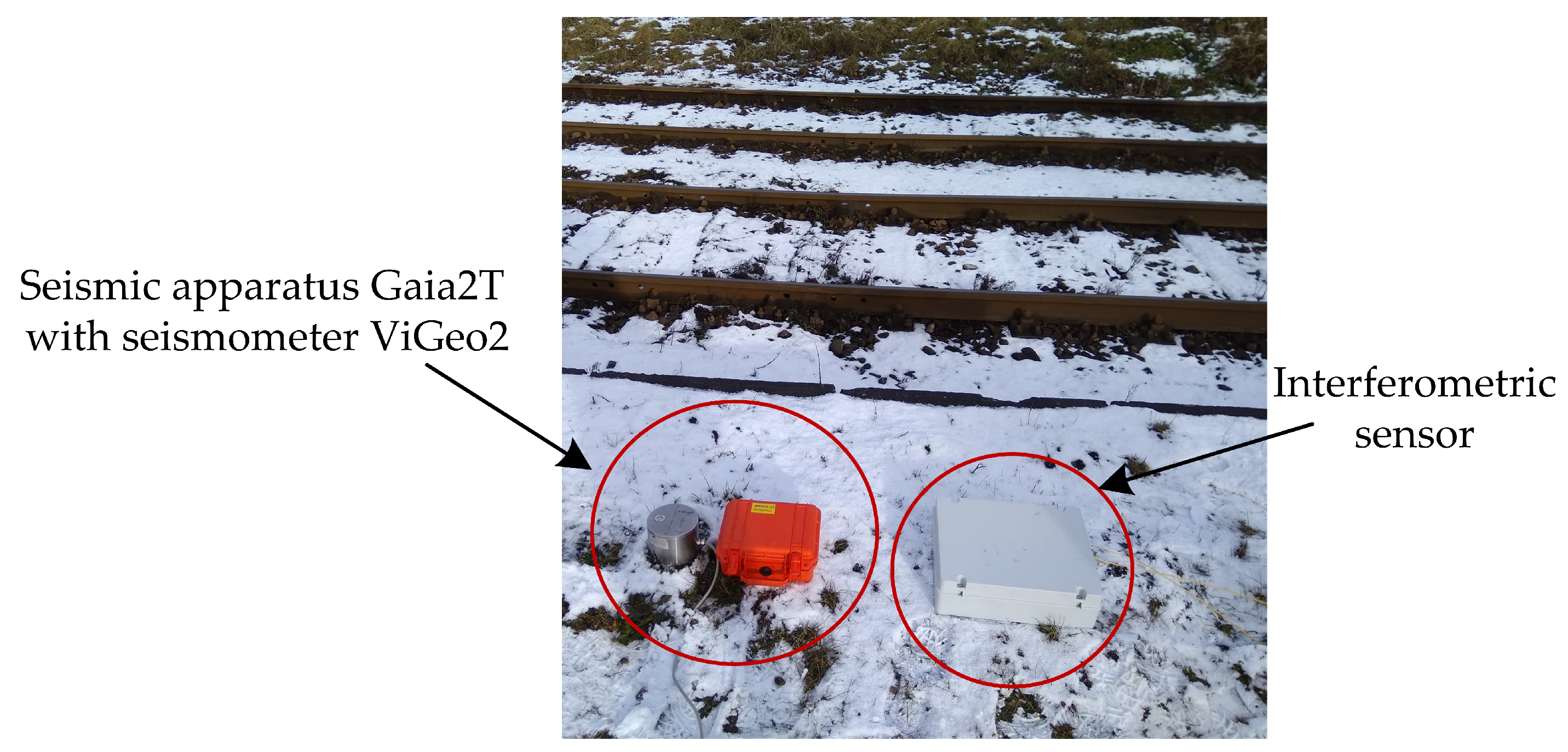
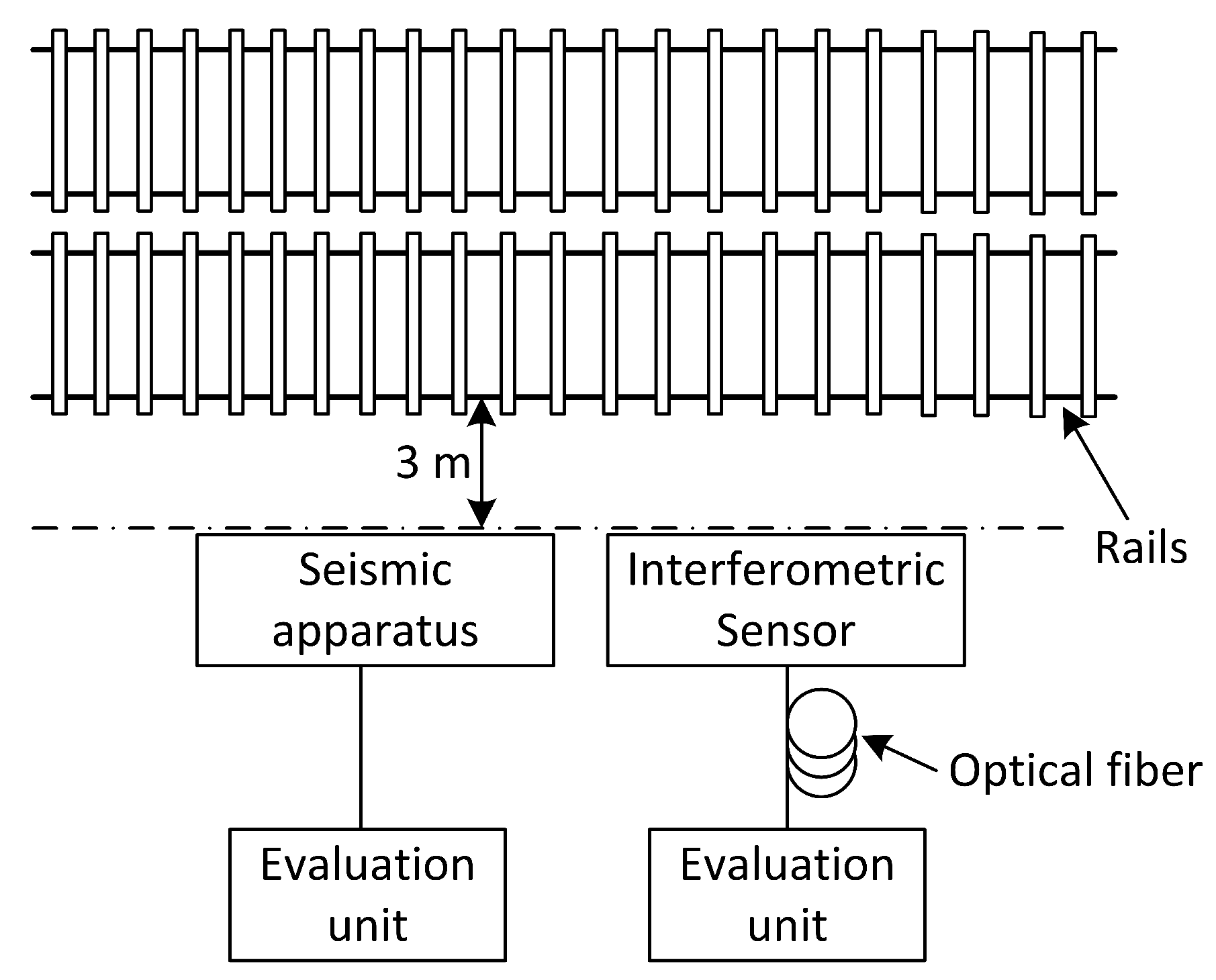
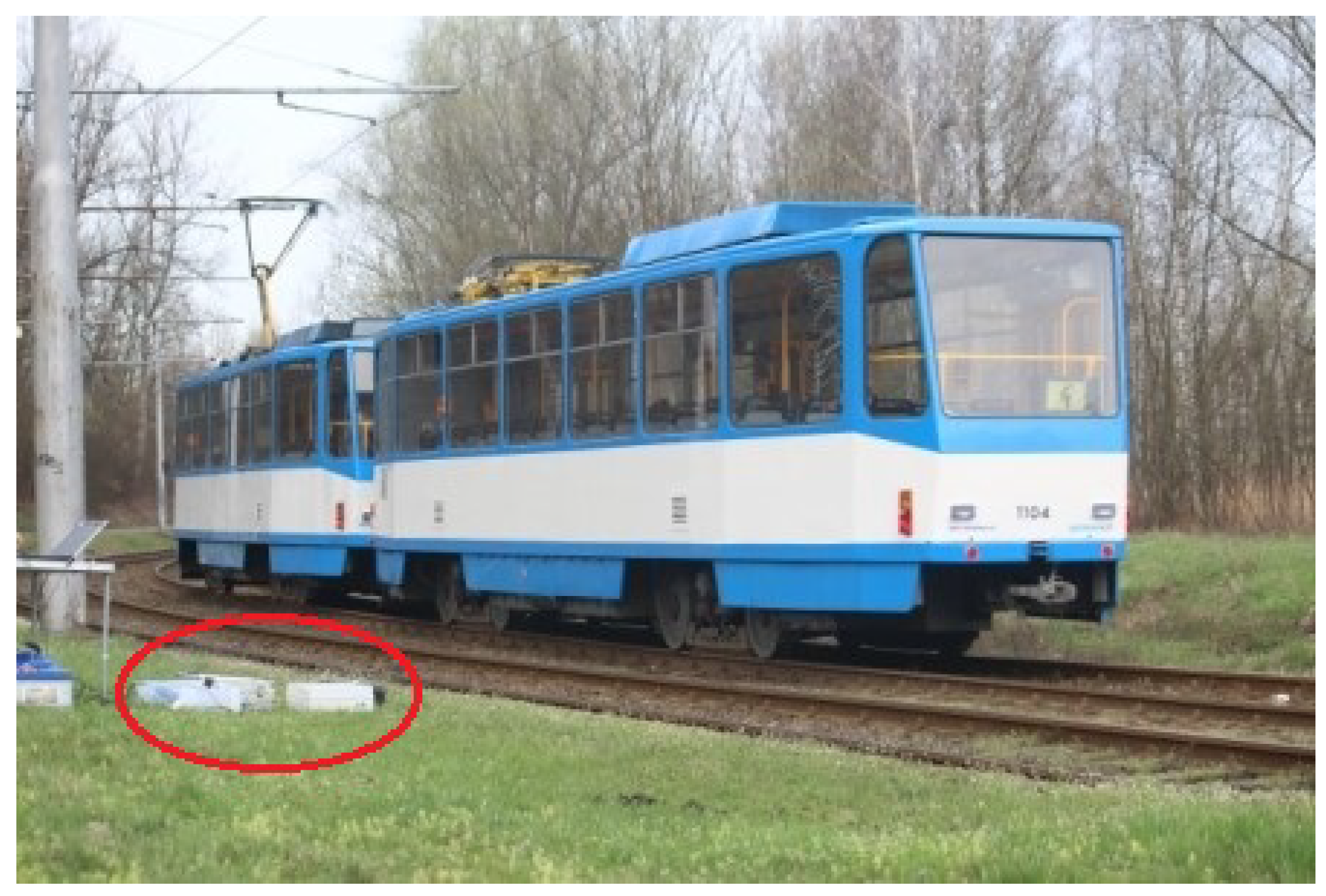
4. Experimental Setup

Various types of trams were analyzed during the experimental measurements on both the nearer track (travel in one direction) and the more distant track (travel in the opposite direction). No adverse effect created by the sensor’s distance (more distant track) (seismic equipment Gaia 2T and interferometric sensor) from the track on its detection capacity was observed, nor was the measured frequency spectrum adversely affected, as the results presented below demonstrate. Both sensors were placed 3 m (Figure 8 and Figure 9) from the (nearer) rails, as the distance of the sensor from the rails is defined (in the Czech Republic) by the so-called hazardous area of traction lines according to standard CSN-34-1500 ed.2 from 2011 [50]. Practical measurements were taken in the city of Ostrava on Podzamci Street, GPS coordinates 49.8293328N, 18.2975139E.

The range of vehicle speeds measured was 15–65 kph, in accordance with the limits given by rail signs. The total measurement time was performed over ten separate days. Measurements were carried out in two different climatic conditions: winter (temperatures below 0 ${}^{\circ }$C) and summer (temperatures above 25 ${}^{\circ }$C). Figure 9 shows the measurement methodology. Statistical analysis of the detection success rate was based on a total of 769 measurements, i.e., the number of trams that passed.

5. Results

This section statistically summarizes the measured results. For a better visual comparison, the time and frequency records obtained simultaneously from the interferometric sensor and Gaia 2T seismic station were compared graphically for a single passing light rail vehicle identified as CKD T6A5, Czech produced, with two cars (Figure 10).

Figure 11a shows an example of a time record of the passing tram measured by the interferometric sensor, while Figure 11b shows a time record of the passing tram measured by the Gaia 2T seismic station. Analysis and evaluation of the measured data identified the individual axles of the passing tram as individual maximums (Figure 11, marked in red). These maximums can be seen in all the recorded measurements and correspond to the recordings obtained by the Gaia 2T seismic equipment. This standard seismic station can be used as a reference for calculating rolling stock axles, as demonstrated in [51]. The voltage amplitude (V) corresponds to the resulting intensity of optical radiation on the photo detector and is proportionate to the size of the phase change between the light beams and the measuring and reference arms of the interferometric sensor.

Figure 12a shows the frequency spectrum of the passing tram measured by the interferometric sensor, while Figure 12b shows an example of the frequency spectrum measured by the seismic station.

Table 2. Summary of tram vehicle detection measurements.

Measuring Day	Year Period	Number of Passes (Direction/Opposite)	Detection Success, Interferometric Sensor (%)	Detection Success, Seismic Station (%)
1	winter	40/39	100	100
2	winter	36/38	100	100
3	winter	37/36	100	100
4	winter	38/37	100	100
5	winter	36/38	100	100
6	summer	41/39	100	100
7	summer	38/40	100	100
8	summer	39/38	100	100
9	summer	37/39	100	100
10	summer	42/41	100	100

summarizes all measurements and the success of detection in both sensor types. The measurements show that trams were detected at 100% efficiency in all measurements. This fact is an essential premise for the possibility of using an interferometric sensor as a tool to monitor the vibration-acoustic responses of the environment beneath passing trams in terms of time and frequency.

A significant agreement was seen in the measured data for the time records and frequency spectra between both items of equipment (the seismic station and the interferometric sensor) (

Table 3. Summary of the results of measured frequencies from both devices with regard to the type of tram.

Tram Type	Number of Passes	Bandwidth (Hz)		Dominant Component (Hz)
		Seismic Station	Interferometric Sensor	Seismic Station	Interferometric Sensor
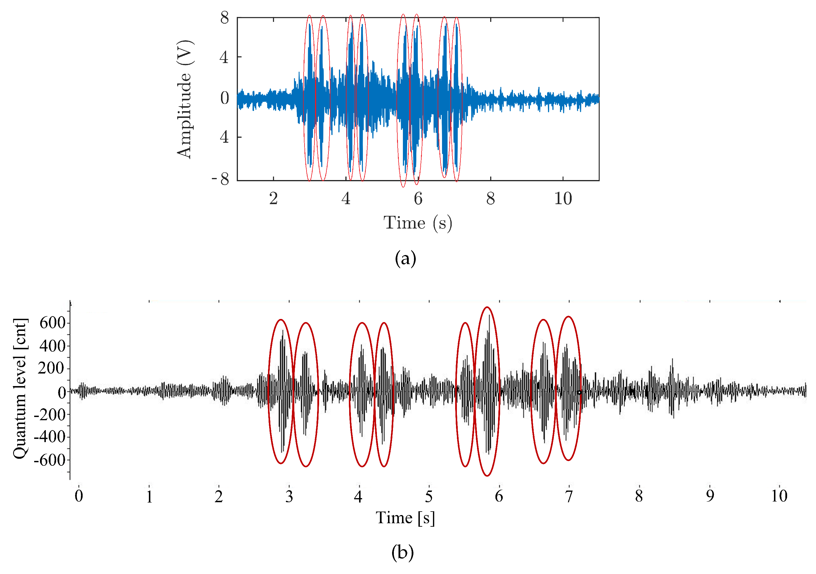
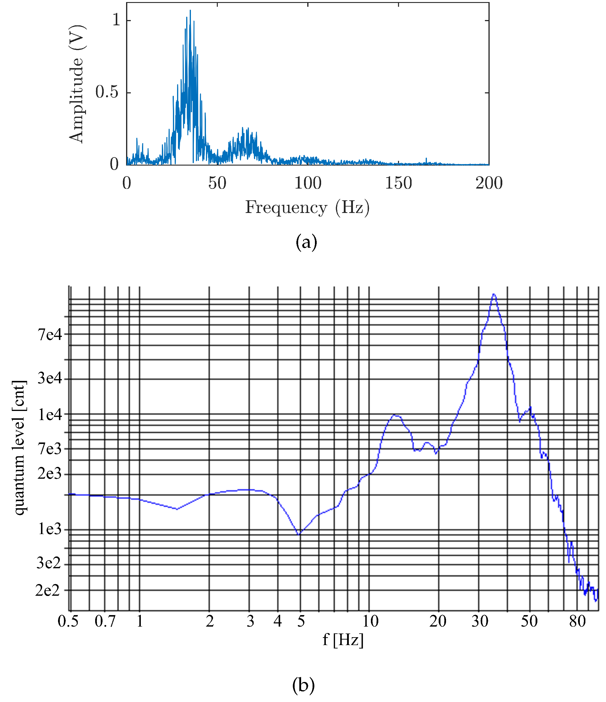
Vario LFR	176	20–45	24–46	35–38	32–36
CKD T3	162	22–48	20–48	35–36	36–38
Inekon LTM 10.08	158	25–45	24–48	34–36	32–38
Inekon 2001 TRIO	145	25–55	20–50	32–36	33–38
CKD T6A5	128	20–45	22–50	34–35	34–36

). The positions of maximums in the time records representing individual tram axles were identical and corresponded to the number of cars and axles of the passing trams. The character of frequency spectra differed significantly only with regard to the type of tram. In general, a prevailing frequency range between 15 and 50 Hz was observed. A marked maximum in the area around 35 Hz was repeatedly present in the spectra. The same frequencies were proven independently by the fiber-optic sensor and seismic station. With regard to direction of travel, more significant changes in the spectra were recorded, which were caused by the speed of trams being constant in both directions and the proximity of both tracks. Table 3 compares the results of frequencies obtained from both devices with regard to the type of tram.

6. Discussion

A basic limitation in fiber-optic interferometry is associated with the design of the reference channel in the fiber-optic interferometer. The basis of interferometry is measuring the differences between signals in the measurement (sensor) and reference channels. The reference channel of an interferometer must be designed in a way that allows all unwanted signals to be eliminated. Background noise (unwanted signals) originate from thermal phenomena, mechanical changes, and other factors. Precise positioning of the reference channel is also highly critical to a sensor’s sensitivity, which must be carefully taken into account in fiber-optic interferometer design [52,53,54,55].

The error signal caused by the instability of light polarization and external influences (temperature) can be described as a slow change in phase with a frequency that is one order of magnitude less than the lowest frequency of the desired signal. Because of this difference, the first-order high-pass (HP) filter with a corner frequency of 2 Hz can be used. For the compensation of unwanted signals like snow, rain, wind, and other environmental influences, we can use a software filtration method.

As our sensor system uses G.652 optical fibers, which are widely used in current telecommunications systems, they can be readily connected to existing telecommunications networks (dark cables around tracks) without the need for any additional transducers. The low attenuation of single-mode fibers (0.2 dB/km) allows the evaluation unit to be placed several km from the sensor (the evaluation unit is much more expensive than the sensor; therefore, remote evaluation or placing the evaluation unit at a safe location is a clear advantage).

Optical fibers are currently being increasingly dedicated to communications applications. However, there is also a global trend in which many research and industrial corporations are applying optical fiber sensors in the monitoring or recording of various physical phenomena in transportation. For an example of the application of optical sensors in monitoring underground traffic, please see [56].

An essential difference between a standard seismic station and the alternative in the form of a fiber-optic interferometric sensor is primarily the price of the equipment, which is an order higher for seismic stations by thousands of U.S. dollars [8,9,10]. The price of an interferometric sensor based on classic telecommunications fibers and affordable materials is only hundreds of U.S. dollars for a prototype. The paper highlights the possibility of using a fiber-optic interferometric sensor as a suitable alternative to a seismic station. In the case of a seismic station, we work with compact, calibrated, autonomous equipment mainly intended for continuous field seismic measurements. There is no need for an external source, access to computers, permanent operation, etc. By contrast, the sensor we tested is a developed experimental device. We now expect a series of experiments to improve partial parameters, such as sensitivity, dimensions, optimization of materials, etc.

Another difference is in measurement results. A seismic station provides data on mass point vibration (a velocity or acceleration amplitude) in three mutually perpendicular directions (vertical, horizontal, radial, and horizontal-transversal), while the fiber-optic interferometer provides a single wave image showing the prevailing direction of vibrations. Both differences are due to the structure of the equipment and the philosophy of the approach, where a seismic station can be considered conventional equipment and the optical interferometer as a non-conventional alternative. Despite these limitations, interesting results were obtained, which agreed significantly, both in amplitude and frequency. Amplitude showed that individual tram vehicle axles were clearly detected. Similar results can be expected, for example in monitoring the dynamic response beneath passing trains, in which it should be possible to read the number of passing cars of long freight trains, which burden their surroundings most with dynamic load, except for high-speed trains, according to the records. Frequency showed an agreement in the bandwidth, which generally corresponded to rail transport, and in the maximum peaks for individual types of tram cars. We can see the highest potential of the optical interferometer in measuring frequencies, another logical step being the implementation of experimental measurements similar to the scheme presented, but in a building. This is also another task of seismic engineering, i.e., assessing the dynamic response of building structures.

The results published in this paper show the possible use of this type of sensor in monitoring selected rail transport parameters (detecting vehicles, measuring vehicle speed with two sensors, etc.). In order to detect trams passing by simultaneously (nearer vs. more distant track), individual vehicles can be distinguished in a frequency data analysis. Problems in operational reliability occur because of a significant increase in electromagnetic disturbance from the new technologies used in modern traction units and the signal contamination caused by the return traction current in rails. Another problem with electrical detection systems is due to their low resistance to influences or damage caused by an atmospheric discharge, such as lightning at a nearby railway facility. In installations with metallic interconnections, undesirable conductive loops are formed (completed) via electrically-conductive circuits and create very difficult conditions to alleviate their undesirable influences or damage. With our proposed system design based on optical fibers, these problems can be eliminated due to the fact that optical fibers are dielectric in nature. However, follow-up and long-term practical tests are required, according to which the sensor can be optimized for potential practical use. A part of the solutions presented here is currently protected by copyright certificate (Utility Model Number 30137 and Patent License Number 306992).

7. Conclusions

This publication describes the use of an interferometric sensor based on the Mach–Zehnder interferometer as an alternative to current standard seismic stations. The presented sensor operates with single-mode telecommunications optical fibers according to standard G.652.D., with a wave length of 1550 nm and a radiation source with a power output in the order of milliwatts. The paper compared original results based on an evaluation of long-term time records. A total of 769 passes was recorded for various types of tram over five months of practical measurements under various climatic conditions. The fiber-optic sensor detected all vehicles at a 100% rate, and the recorded results were compared to the results from a standard seismic station. Amplitude and especially frequency significantly agreed in the results from both items of equipment. Amplitude showed that all tram vehicle axles were detected in individual time records. Frequency showed an agreement in the bandwidth, generally corresponding to rail transport of individual types of tram. The results published in this paper show a potential use for this type of sensor in monitoring selected rail transport parameters as an alternative to existing conventional sensors. The primary reason for reducing the use of conventional sensors is the electromagnetic interferences generated by the new traction drives in rail vehicles and signal contamination caused by the return traction current in rails.

References

- Lopez-Higuera, J.M. Handbook of Optical Fiber Sensing Technology; Wiley: New York, NY, USA, 2002; p. 828. ISBN 978-0-471-82053-6. [Google Scholar]
- Halgamuge, M.N.; Abeyrathne, C.D.; Mendis, P. Measurement and analysis of electromagnetic fields from trams, trains and hybrid cars. Radiat. Prot. Dosim. 2010, 14. [Google Scholar] [CrossRef] [PubMed]
- Thompson, D. Railway Noise and Vibration; Elsevier Science: Amsterdam, The Netherlands, 2009; p. 536. ISBN 978-008045147-3. [Google Scholar]
- BSI Group. BS ISO 4866:2010 Mechanical Vibration and Shock, Vibration of Fixed Structures, Guidelines for the Measurement of Vibrations and Evaluation of Their Effects on Structures; BSI Group: London, UK, 2010. [Google Scholar]
- Zou, C.; Wang, Y.; Moore, J.A.; Sanayei, M. Train-induced field vibration measurements of ground and over-track buildings. Sci. Total Environ. 2017, 575, 1339–1351. [Google Scholar] [CrossRef] [PubMed]
- Degrande, G.; Schillemans, L. Free field vibrations during the passage of a thalys high-speed train at variable speed. J. Sound Vib. 2001, 247, 131–144. [Google Scholar] [CrossRef]
- Galvín, P.; Domínguez, J. Experimental and numerical analyses of vibrations induced by high-speed trains on the Cordoba-Malaga line. Soil Dyn. Earthq. Eng. 2009, 29, 641–657. [Google Scholar] [CrossRef]
- GeoSIG. Available online: https://www.geosig.com (accessed on 10 October 2018).
- Nitro Consult. Available online: https://www.nitroconsult.com (accessed on 5 October 2018).
- Guideline GEO, Abem, Mala. Available online: https://www.guidelinegeo.com (accessed on 13 October 2018).
- Busca, G.; Cigada, A.; Mazzoleni, P.; Zappa, E. Vibration Monitoring of Multiple Bridge Points by Means of a Unique Vision-Based Measuring Systém. Exp. Mech. 2014, 54, 255–271. [Google Scholar] [CrossRef]
- Wada, A.; Ikum, K.; Tanaka, S.; Takahashi, N. Experimental investigation of dynamic characterisitics of wavelength of DFB-LD for FBG-FPI vibration sensor based on wavelength-to-time mapping. In SPIE—International Society for Optical Engineering; SPIE: Beijing, China, 2012. [Google Scholar]
- Beben, D.; Anigacz, W. Dynamic testing of railway metal culvert using geodetic methods. In Proceedings of the MATEC Web of Conferences, Oravsky Haj-Trstena, Slovakia, 21–25 May 2017. [Google Scholar] [CrossRef]
- Nedoma, J.; Zboril, O.; Fajkus, M.; Zavodny, P.; Kepak, S.; Bednarek, L.; Martinek, R.; Vasinek, V. Fiber optic system design for vehicle detection and analysis. In SPIE—The International Society for Optical Engineering; SPIE: Brussels, Belgium, 2017. [Google Scholar]
- Nedoma, J.; Fajkus, M.; Martinek, R.; Mec, P.; Novak, M.; Jargus, J.; Vasinek, V. Fiber-optic sensor for monitoring a density of road traffic. In SPIE—The International Society for Optical Engineering; SPIE: Warsaw, Poland, 2017. [Google Scholar]
- Nedoma, J.; Fajkus, M.; Martinek, R.; Mec, P.; Novak, M.; Bednarek, L.; Vasinek, V. Fiber-optic sensor based on Mach-Zehnder interferometer for securing entrance areas of buildings. In SPIE—The International Society for Optical Engineering; SPIE: Warsaw, Poland, 2017. [Google Scholar]
- Araya, A.; Takamori, A.; Morii, W.; Miyo, K.; Ohashi, M.; Hayama, K.; Uchiyama, T.; Miyoki, S.; Saito, Y. Design and operation of a 1500-m laser strainmeter installed at an underground site in Kamioka, Japan. Earth Planets Sp. 2017, 69. [Google Scholar] [CrossRef] [Green Version]
- Papp, B.; Donno, D.; Martin, J.E.; Hartog, A.H. A study of the geophysical response of distributed fiber optic acoustic sensors through laboratory-scale experiments. Geophys. Prospect. 2017, 65, 1186–1204. [Google Scholar] [CrossRef]
- Udd, E. Fiber Optic Sensors for Infrastructure Applications. Oregon State Library. Available online: http://www.oregon.gov/ODOT/TD/TP_RES/ResearchReports/FiberOpticSensors.pdf (accessed on 21 October 2017).
- Crail, S.; Reichel, D.; Schreiner, U.; Lindner, E.; Habel, W.R.; Hofmann, D.; Basedau, F.; Brandes, K.; Barner, A.; Ecke, W.; et al. Strain monitoring of a newly developed precast concrete track for high speed railway traffic using embedded fiber-optic sensors. Proc. SPIE 2002, 4694. [Google Scholar] [CrossRef]
- Siemens, A.G. Rail Contacting Device in Railway Systems, Particularly for Axle Counting Devices. DE Patent 3537588 A1, 22 October 1985. [Google Scholar]
- Bledin, A.G. Contact Fiber Optic Impact Sensor. U.S. Patent 6,144,790 A, 7 November 2000. [Google Scholar]
- Kepak, S.; Cubik, J.; Zavodny, P.; Siska, P.; Davidson, A.; Glesk, I.; Vasinek, V. Fiber optic track vibration monitoring system. Opt. Quantum Electron. 2016, 48, 354. [Google Scholar] [CrossRef]
- Kepak, S.; Cubik, J.; Zavodny, P.; Hejduk, S.; Nedoma, J.; Davidson, A.; Vasinek, V. Fiber optic portable rail vehicle detector. In SPIE—The International Society for Optical Engineering; SPIE: Jasna, Slovakia, 2016; Volume 10142. [Google Scholar]
- Soltys, A.; Pyra, J.; Winzer, J. Analysis of the blast-induced vibration structure in open-cast mines. J. Vibroeng. 2017, 19, 409–418. [Google Scholar] [CrossRef]
- Kondela, J.; Pandula, B. Timing of quarry blasts and its impact on seismic effects. Acta Geodyn. Geomater. 2012, 9, 155–163. [Google Scholar]
- Lednicka, M.; Kalab, Z. Vibration response of the waste rock dump in open pit mine caused by blasting operation. Acta Montan. Slov. 2015, 20, 71–79. [Google Scholar] [CrossRef]
- Stolarik, M.; Pinka, M. Analysis of transfer coefficients based on seismic measurements in three tunnels. In Proceedings of the International Multidisciplinary Scientific GeoConference Surveying Geology and Mining Ecology Management, Albena, Bulgaria, 17–26 June 2013. [Google Scholar]
- Sanayei, M.; Maurya, P.; Moore, J.A. Measurement of building foundation and ground-borne vibrations due to surface trains and subways. Eng. Struct. 2013, 53, 102–111. [Google Scholar] [CrossRef]
- Connoly, D.P.; Kouroussis, G.; Woodward, P.K.; Alves Costa, P.; Verlinden, O.; Forde, M.C. Field testing and analysis of high speed rail vibrations. Soil Dyn. Earthq. Eng. 2014, 67, 102–118. [Google Scholar] [CrossRef] [Green Version]
- Stolarik, M.; Pinka, M.; Marsalek, J. Analysis of load of the tunnel definitive lining due to vibrations of various sources. Adv. Mater. Res. 2014, 1020, 429–434. [Google Scholar] [CrossRef]
- Stolarik, M.; Pinka, M. Seismic impact of the railway on the geotechnical constructions. In IOP Conference Series: Materials Science and Engineering; IOP: Prague, Czech Republic, 2017. [Google Scholar]
- Stolarik, M.; Pinka, M.; Mohyla, M. Dynamic load due to the tram in urban area. In Proceedings of the International Multidisciplinary Scientific GeoConference Surveying Geology and Mining Ecology Management, Albena, Bulgaria, 29 June–5 July 2017; pp. 271–278. [Google Scholar] [CrossRef]
- Lednicka, M. Elaboration of ground motion directivity in undermined area based on seismic noise measurement. In Proceedings of the International Multidisciplinary Scientific GeoConference Surveying Geology and Mining Ecology Management, Albena, Bulgaria, 18–24 June 2015; pp. 815–822. [Google Scholar]
- Jwa, Y.; Sonh, G. Kalman Filter Based Railway Tracking from Mobile Lidar Data. In Proceedings of the ISPRS Annals of Photogrammetry, Remote Sensing and Spatial Information Sciences, La Grande Motte, France, 28 September–3 October 2015; pp. 159–164. [Google Scholar] [CrossRef]
- Leslar, M.; Gordon, P.; McNease, K. Using mobile lidar to survey a railway line for asset inventory. In Proceedings of the ASPRS 2010 Annual Conference, San Diego, CA, USA, 26–30 April 2010. [Google Scholar]
- Klug, F.; Lackner, S.; Lienthart, W. Monitoring of Railway Deformations using Distributed Fiber Optic Sensors. In Proceedings of the Joint International Symposium on Deformation Monitoring, Vienna, Austria, 30 March–1 April 2016. [Google Scholar]
- Lopez-Pacheco, M.G.; Saanchez-Fernaandez, L.P.; Molina-Lozano, H.M. A method for environmental acoustic analysis improvement based on individual evaluation of common sources in urban areas. Sci. Total Environ. 2014, 468–469, 724–737. [Google Scholar] [CrossRef]
- Goodwin, E.P.; Wyant, J.C. Field guide to interferometric optical testing. In SPIE Field Guides, Bellingham, Wash, 2006; SPIE Press: Washington, DC, USA, 2006; ISBN 9780819465108. [Google Scholar]
- Todd, M.D.; Seaver, M.; Bucholtz, F. Improved, operationally-passive interferometric demodulation method using 3 × 3 coupler. Electron. Lett. 2002, 38. [Google Scholar] [CrossRef]
- Ferreira, M.F.S. Optical Fibers: Technology, Communications and Recent Advances (2017) Optical Fibers: Technology, Communications and Recent Advances; Nova Science Pub Inc.: Hauppauge, NY, USA, 2017; pp. 1–263. [Google Scholar]
- Donlagic, D.; Hanč, M. Vehicle axle detector for roadways based on fiber optic interferometer (2003). In SPIE—The International Society for Optical Engineering; SPIE: San Diego, CA, USA, 2003; pp. 317–321. [Google Scholar]
- Cubik, J.; Kepak, S.; Doricak, J.; Vasinek, V.; Jaros, J.; Liner, A.; Papes, M.; Fajkus, M. The usability analysis of different standard single-mode optical fibers and its installation methods for the interferometric measurements. Adv. Electr. Electron. Eng. 2013, 11, 535–542. [Google Scholar] [CrossRef]
- Kepak, S.; Cubik, J.; Doricak, J.; Vasinek, V.; Liner, A.; Siska, P.; Papes, M. The arms arrangement influence on the sensitivity of Mach–Zehnder fiber optic interferometer. Opt. Sens. 2013. [Google Scholar] [CrossRef]
- Nedoma, J.; Fajkus, M.; Martinek, R.; Zboril, O.; Bednarek, L.; Novak, M.; Witas, K.; Vasinek, V. Analysis of the detection materials as resonant pads for attaching the measuring arm of the interferometer when sensing mechanical vibrations. Opt. Sens. 2017. [Google Scholar] [CrossRef]
- Nedoma, J.; Fajkus, M.; Martinek, R.; Bednarek, L.; Zabka, S.; Hruby, D.; Jaros, J.; Vasinek, V. Impact of fixing materials on the frequency range and sensitivity of the fiber-optic interferometer. Fiber Opt. Sens. Appl. XIV 2017. [Google Scholar] [CrossRef]
- Cubik, J.; Kepak, S.; Fajkus, M.; Zboril, O. Fixing methods for the use of optical fibers in interferometric arrangements. In Proceedings of the 20th Slovak-Czech-Polish Optical Conference on Wave and Quantum Aspects of Contemporary Optics, Jasna, Slovakia, 5–9 September 2016. [Google Scholar] [CrossRef]
- French, A.P. In Vino Veritas: A study of wineglass acoustics. Am. J. Phys. 1982, 51, 688–694. [Google Scholar] [CrossRef]
- Wiszniowski, J.; Wiejacz, P. Program SWIP; Institute of Geophysics, Polish Academy of Sciences: Warszaw, Poland, 2003; p. 36. [Google Scholar]
- CSN 34 1500 ED.2 (341500)-Drazni Zarizeni-Pevna Trakcni Zarizeni-Predpisy pro Elektricka Trakcni Zarizeni. Available online: http://www.technicke-normy-csn.cz/341500-csn-34-1500-ed-2_4_84547.html (accessed on 3 October 2018).
- Kouroussis, G.; Pauwels, N.; Brux, P.; Conti, C.; Verlinden, O. A numerical analysis of the influence of tram characteristics and rail profile on railway traffic ground-borne noise and vibration in the Brussels Region. Sci. Total Environ. 2014, 482–483, 452–460. [Google Scholar] [CrossRef] [PubMed]
- Born, M.; Wolf, E. Principles of Optics: Electromagnetic Theory of Propagation, Interference and Diffraction of Light, 6th ed.; Cambridge University Press: Pergamon, Turkey, 1980; p. 836. ISBN 978-0-08-026482-0. [Google Scholar]
- Born, M.; Wolf, E. Principles of Optics: Electromagnetic Theory of Propagation, Interference and Diffraction of Light, 7th ed.; Cambridge University Press: New York, NY, USA, 1999; ISBN 05-216-4222-1. [Google Scholar]
- Kipnis, N. History of the Principle of Interference of Light; Birkhäuser: Basel, Switzerland, 1991; ISBN 978-303-4886-529. [Google Scholar]
- Gundersen, P.E. The Handy Physics Answer Book; Visible Ink Press: Detroit, MI, USA, 1999; ISBN 15-785-9058-2. [Google Scholar]
- Optical-Fiber Sensing Technology Offers Double Railway Monitoring. South China Morning Post. Available online: http://www.scmp.com/presented/news/topics/polyu-innovating-better-world/article/2065348/optical-fiber-sensing-technology (accessed on 21 October 2017).