Improvement in Classification Performance Based on Target Vector Modification for All-Transfer Deep Learning

Abstract

This paper proposes a target vector modification method for the all-transfer deep learning (ATDL) method. Deep neural networks (DNNs) have been used widely in many applications; however, the DNN has been known to be problematic when large amounts of training data are not available. Transfer learning can provide a solution to this problem. Previous methods regularize all layers, including the output layer, by estimating the relation vectors, which are then used instead of one-hot target vectors of the target domain. These vectors are estimated by averaging the target domain data of each target domain label in the output space. This method improves the classification performance, but it does not consider the relation between the relation vectors. From this point of view, we propose a relation vector modification based on constrained pairwise repulsive forces. High pairwise repulsive forces provide large distances between the relation vectors. In addition, the risk of divergence is mitigated by the constraint based on distributions of the output vectors of the target domain data. We apply our method to two simulation experiments and a disease classification using two-dimensional electrophoresis images. The experimental results show that reusing all layers through our estimation method is effective, especially for a significantly small number of the target domain data.

1. Introduction

Deep learning has been widely used due to its advanced performance and automatic feature extraction. Training deep neural networks (DNNs) requires a large amount of training data. In medical image analysis fields where privacy and security concerns exist, the proper collection of training data can be challenging. Conventional training methods address this problem by applying transfer learning [1,2].

Transfer learning reuses source domain knowledge to solve a new task in the target domain [3]. Transfer learning can be divided into three approaches: supervised, semi-supervised, and unsupervised learning. Unsupervised and semi-supervised learning approaches assume that the target domain labels are the same as the source domain labels [4,5]. However, in the application to the medical field, and in others as others as well, it is difficult to collect data where the source domain and target domain use the same labels. In addition, many semi-supervised and unsupervised learning methods have to train DNNs by using the source and target domains at the same time. It is difficult to upload the target domain data outside of a hospital and prepare a sufficient computer environment, especially for small- and medium-sized hospitals. This paper addresses tasks to classify diseases using proteome data for these small- and medium-sized hospitals. Therefore, we argue that the supervised transfer learning approach fits the clinical demand in this target environment.

Supervised transfer learning has been widely used in the field of computer vision [6,7,8]. Given the labeled source/target domain data, first, many methods train a DNN using the source domain data. Then, a second DNN is constructed based on the target domain data by reusing the hidden layers of the first DNN to set the initial values for the network structure and weights. This approach has the advantages that the DNN for the source domain can be constructed prior to obtaining and preparing the target domain data and it is not necessary to retain the source domain data. However, there is a risk of poor classification performance owing to the random initial values of weights (and biases) that are not reused. This can occur when these parameters are trained on a small amount of target domain data. To avoid this problem, it is important to reuse all layers, including the output (last) layer [2].

To reuse all layers, Sawada et al. [2] proposed the all-transfer deep learning (ATDL) method. ATDL trains the first DNN to solve the source domain task. It then averages the target domain data of each target domain label in the output space, which has the same dimension as the number of source domain labels. This computation is conducted in the output layer, which is thrown away by conventional methods [6,7,8]. In [2], this vector is called the relation vectors (Section 2.2.1). Following that, the second DNN is initialized by the first DNN and optimized using the estimated relation vectors instead of the one-hot target vectors. By using this method, it is not necessary to throw away the output layer. The main difference between the ATDL and other supervised transfer learning methods is that the ATDL can use the first DNN to regularize all parameters of a second DNN. This means that the ATDL can reduce the risk of the local optimal solution caused by the random initial values of the non-transferred parameters. However, their estimation cannot consider the relation between the target domain labels. To improve the classification performance, the appropriate configuration of relation vectors must be considered in regard to this relation.

This paper proposes a relation vector modification based on constrained pairwise repulsive forces. A strong pairwise repulsive force between the relation vectors is introduced to produce a large distance (Section 3.1). In addition, to mitigate the risk of divergence, we constrain these vectors to be close to the distributions computed on the target domain data in the output space (Section 3.2). By using this modification, the distance between the relation vectors can be maximized without the risk of divergence.

Our method was applied to an actual disease classification problem using two-dimensional electrophoresis (2-DE) images [2,9]. These 2-DE images were used as principles of proteomics, which is a field of study that has attracted much attention as a step beyond genomics. However, collecting 2-DE images of patients is still difficult due to privacy and security concerns. This clearly indicates the need for a method that can succeed using only a small amount of training data.

The contributions of this paper are as follows:

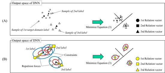
• We propose a relation vector modification for ATDL with constrained pairwise repulsive forces between relation vectors.
• Experimental results showed that our method is effective, especially when the target domain data are significantly small.
• We also showed that the distance between the relation vectors relates to the classification performance.

2. Related Work

In supervised transfer learning, a two-phase approach has been widely used [6,8,10,11].

In [6], the first DNN was constructed based on the source domain. The second DNN, for the target domain task, was constructed by reusing all the hidden layers from the first DNN as the initial values, and all layers were then optimized. The performance of this method was better than the performance of other methods, in which the reuse of a part of the hidden layers breaks their co-adaptation [10]. To improve this method, a two-phase know-how [12], where the first trains only the output layer and all layers are then optimized, is proposed, although it has not been published yet.

In [11], the output layer of the second DNN was constructed by a linear SVM and all hidden layers were frozen. In [13], the output layer of the second DNN was constructed by the pseudo-inverse, which is a linear classification approach instead of a linear SVM. In [8], the output layer of the first DNN was removed and two layers, an additional adaptation layer and a new output layer, were added. The additional adaptation layer compensated for the different statistics of the source and target domains. This method also froze the hidden layers.

These methods had to train the last parameters (the weights and biases connecting the output layer and the highest hidden layer) of the second DNN from scratch [6,8,11]. On the other hand, in [14], the authors proposed an all-layer transfer method that can execute when the source and target domain data have the same label. However, their methods do not apply when the target domain labels have meanings different from those of the source domain labels. ATDL [2] can solve this problem.

2.1. All-Transfer Deep Learning

In this section, we explain how to estimate the relation vectors according to the framework of all-transfer deep learning (ATDL) [2].

2.2. Outline

The ATDL is one of the supervised transfer DNN learning methods that can reuse all layers, including the output layer. An outline of the ATDL training process is shown in Figure 1. Given the labeled source and target domain data, the ATDL trains a DNN to solve the task within the source domain (Figure 1A). The ATDL then estimates the output vectors of each target vector by feeding them into the DNN, which was trained on the source domain data (Figure 1B). Next, it estimates the relation vectors of each target domain label by averaging. Finally, all parameters are optimized in such a way that the variance between the output and relation vectors is sufficiently small (Figure 1C). By using the steps in Figure 1B,C, a second DNN can be optimized with the regularization of all parameters. This means that ATDL enables the second DNN to avoid the local optimal solution caused by the random initial values of the non-transferred weights. Details are described in the following section.

2.2.1. The First DNN Construction (Figure 1A)

The ATDL constructs the first DNN by minimizing the following function:

$$L^s\alpha =\sum _i^{N^s}\left|\right|{\mathit{y}}_i^s-\varphi \left({\mathit{x}}_i^s\right){\left|\right|}^2$$

(1)

where $N^s=N^s\left(1\right)+N^s\left(2\right)+\cdots +N^s\left(D_y^s\right)$ is the amount of source domain data, $D_y^s$ is the number of source domain labels, ${\mathit{y}}_i^s$ is a $D_y^s$ dimensional one-hot target vector of the i-th source domain data ${\mathit{x}}_i^s$, and $\varphi \left({\mathit{x}}_i^s\right)$ is an output vector of ${\mathit{x}}_i^s$.

2.2.2. Relation Vector Estimation (Figure 1B)

Normally, the target vector of the target domain data, ${\mathit{y}}^t$, is represented by the one-hot vector, whose dimension is the number of target domain labels, $D_y^t$. However, this one-hot representation does not apply to the ATDL where the target domain labels have meanings different from those of the source domain labels. This frequently occurs in industrial applications. To address this problem while achieving the reuse of all layers, the ATDL estimates a relation vector ${\mathit{m}}_l\in {\mathbb{R}}^{D_y^s}$ ($l=1,2,\cdots ,D_y^t$) instead of using the one-hot representation.

$${\mathit{m}}_l=\sum _i^{{}_{{}^{N^t\left(l\right)}}}\varphi \left({\mathit{x}}_{i,l}^t\right)$$

(2)

where ${\mathit{x}}_{i,l}^t$ denotes the i-th target domain vector corresponding to the l-th target domain label and $N^t\left(l\right)$ denotes the number of the target domain data of the l-th target domain label ($N^t\left(1\right)+N^t\left(2\right)+\cdots +N^t\left(D_y^t\right)=N^t$).

As described in [2], relation vectors represent the relation between the source and target domains. Namely, the k-th variable $m_l\left(k\right)$ indicates the strength of the relation between the k-th source domain label and l-th target domain label. Examination of the values of relation vectors can indicate which labels of the source domain data are similar to those of the target domain data.

2.2.3. Second DNN Construction (Figure 1C)

After estimating the relation vector $m_l$ (Section 2.2.1), the ATDL sets ${\mathit{m}}_l$ instead of the one-hot target vector ${\mathit{y}}^t$. Then, the ATDL minimizes the following main cost function, which was initialized by the first DNN parameters.

$$L^t=\sum _l^{D_y^t}\sum _i^{N^t\left(l\right)}{\parallel {\mathit{m}}_l-\varphi \left({\mathit{x}}_{i,l}^t\right)\parallel }^2.$$

(3)

By following these steps, we can construct the second DNN, which is to be used for the target domain. In the classification step, it assigns the label of the nearest estimated target vector as the label of the test data.

3. Target Vector Estimation with a Constrained Pairwise Repulsive Force

As described in Section 1, the previously described ATDL could not consider the relation between the relation vectors. Figure 2 shows an example of the configurations of these vectors. As shown in Figure 2A, relation vectors computed by the previous ATDL are close to each other (especially the data of the 1st and 2nd target domain labels). In this case, the classification performance might not be satisfactory. To address this problem, repulsion forces are introduced to provide large distances between the relation vectors under constraints, as shown in Figure 2B. By solving the following equation, we can obtain the l-th modified relation vector ${\mathit{r}}_l^{*}\in {\mathbb{R}}^{D_y^s}$.

$${\left\{{\mathit{r}}_l^{*}\right\}}_{{}_{l=1}}^{{}_{{}_{D_y^t}}}=\underset{\left\{{\mathit{r}}_l\right\}}{\arg \max } p\left({\left\{{\mathit{r}}_l\right\}}_{{}_{l=1}}^{{}_{{}_{D_y^t}}}\right)=\underset{\left\{{\mathit{r}}_l\right\}}{\arg \max }\prod _l^{D_y^t}p\left({\mathit{r}}_l\right)\prod _{l\ne l^{\prime }}p({\mathit{r}}_l,{\mathit{r}}_{l^{\prime }}).$$

(4)

An explanation of each distribution is provided below.

3.1. Repulsion Force

The joint distribution is represented by $p({\mathit{r}}_l,{\mathit{r}}_{l^{\prime }})$, which accounts for the distance between ${\mathit{r}}_l$ and ${\mathit{r}}_{l^{\prime }}$.

$$p({\mathit{r}}_l,{\mathit{r}}_{l^{\prime }})=\frac{1}{Z}exp\left(-\frac{d_{l,l^{\prime }}}{\parallel {\mathit{r}}_l-{\mathit{r}}_{l^{\prime }}{\parallel }^2}\right)$$

(5)

where $d_{l,l^{\prime }}$ is a hyperparameter used to normalize the difference between the distances. In this study, the average distance between $\varphi \left({\mathit{x}}_{i,l}^t\right)$ and $\varphi \left({\mathit{x}}_{j,l^{\prime }}^t\right)$ was set.

3.2. Constraint

To mitigate the risk of divergence of ${\mathit{r}}_l$, $p\left({\mathit{r}}_l\right)$ is used. In this paper, $p\left({\mathit{r}}_l\right)$ is set as follows:

$$p\left({\mathit{r}}_l\right)=\mathcal{N}({\mathit{r}}_l\mid {\mathit{m}}_l,{\mathbf{\Lambda }}_l)$$

(6)

where $\mathcal{N}(.)$ is the Gaussian, and ${\mathbf{\Lambda }}_l$ is the precision matrix obtained by the graphical lasso, which is known to be able to estimate the precision matrix better than the empirical matrix when $N^t\left(l\right)$ is small [15].

3.3. Estimation

In this study, we used the following equation to maximize Equation (4), which is similar to Gibbs sampling [16].

$${\mathit{r}}_l^{\alpha }=\underset{{\mathit{z}}_l}{\arg \max }lnp\left({\mathit{z}}_l\right)\sum _{l\ne l^{\prime }}lnp({\mathit{z}}_l\mid {\mathit{r}}_{l^{\prime }}^{\alpha })$$

(7)

where ${\mathit{r}}_l^{\alpha }$ is the $\alpha$-th sample of the l-th target domain labels $(\alpha =1,2,\cdots )$, ${\mathit{r}}_l^1={\mathit{m}}_l$, and ${\mathit{r}}_1^{\alpha },{\mathit{r}}_2^{\alpha },\cdots$ are given in advance except for ${\mathit{r}}_l^{\alpha }$. We iterate this procedure by cycling through all relation vectors and set ${\left\{{\mathit{r}}_l^{*}\right\}}_{{}_{l=1}}^{{}_{{}_{D_y^t}}}={\left\{{\mathit{r}}_l^{\alpha }\right\}}_{{}_{l=1}}^{{}_{{}_{D_y^t}}}$ after the termination. By using this estimation, we can modify the relation vector from ${\mathit{m}}_l$ to ${\mathit{r}}_l^{*}$ which maximizes the distances under the constraint.

4. Experimental Results

We also compared the performances of conventional transfer learning methods [6,8,11], the two-phase know-how [12], and previous ATDL [2]. These methods have been widely used in the fields of computer vision and medical image recognition. In addition, the performances of the following two methods were compared: full-scratch (termed “Full”) and without the minimization of Equation (3) from our method (termed\“Tuning”).

4.1. Environment and Parameter Settings

We used one CPU (i7 core, 5930K) and one GPU (GeForce GTX TITAN X). Compared to the conventional methods, the computation time of our method only increased by a factor of 1.12 (our method took about 2 h).

We used the grid search method to select hyperparameters. When we conducted the full-scratch methods, combinations from the following hyperparameters provided better results while maintaining the training speed. Therefore, the best parameters were selected as follows: The learning rate was selected from $\{1.0\times {10}^{-3}$, $5.0\times {10}^{-3}$, $1.0\times {10}^{-2}$, and $5.0\times {10}^{-2}\}$. The momentum was selected from $\{0.7,0.99\}$, and the size of the mini-batches was selected from $\{10,100\}$.

The DNN was constructed using a stacked denoising autoencoder (SdA), as performed by Sawada et al. [2]. That DNN was used for all comparisons in the results section, unless stated otherwise. Stochastic gradient descent with momentum, inspired by [17], and Pylearn2 [18] were used for all experiments, with the total iteration set to be the same as the total iteration of full-scratch for all experiments. The numbers of epochs were set to 1000 (Section 4.2) and 200 (Section 4.3). The first DNNs were confirmed to not overfit when using the test data (simulations) or ten-fold cross-validation (sepsis classification) of the source domain in advance. It should be noted that these settings described in this section are applied to all methods. In the two-phase know-how, the number of epochs of the first phase were set to 50 (Section 4.2) and 10 (Section 4.3), and the learning rate was set to be smaller than that of the second phase (e.g., $1.0\times {10}^{-3}$ in the first phase and $1.0\times {10}^{-2}$ in the second phase).

4.2. Simulation Experiments

To accurately grasp our novel method’s ability, it is important to start with a small scale environment [19]. In this article, our method was applied to two simulation experiments with respect to changing the size of the target domain data: (1) using CIFAR (Canadian Institute For Advanced Research)-10 database [20] as the source domain and images of an automobile and pedestrian crossings from ImageNet database [21] as the target domain and (2) using SVHN (Street View House Numbers) database [22] as the source domain and MNIST (Modified National Institute of Standards and Technology database) database [23] as the target domain. Task (1) is an example where the source and target domain data comprise color images, while Task (2) is an example of multiclass classification. For Task (2), since the labels of MNIST and SVHN have the same meaning, Mou et al.’s method [14] was also used for comparison. This method, which is also a supervised transfer learning method, can only function when the source and target domain data have the same label.

For Task (1), the number of hidden layers was set to $H=3$; the numbers of dimensions of the h-th hidden layer were set to $D_h=1000$$(h=1,2,3)$, $D_y^s=10$, $D_y^t=2$; the size of the source domain data was set to $N^s$ = 50,000. For target test data, 750 images of automobiles and 750 of pedestrian crossings were used. For Task (2), parameters were set to $H=3$, $D_y^s=10$, $D_y^t=10$, $D_h=100$, and $N^s$ = 73,257, and the SVHN images were converted to gray-scale. For the target test data, 10,000 images from MNIST were used. The target domain data dimensions of Tasks (1) and (2) were both set to match the dimensions of the source domain data. In addition, these architectures were experimentally determined beforehand.

Table 1. Classification performances of (A) automobile and pedestrian crossings and (B) MNIST. The red bold is the best performance of each evaluation. The black bold is the second best performance.

(A)
${\mathit{N}}^{\mathit{t}}$	400	800	1200	1500
[6]	0.753	0.778	0.790	0.781
[8]	0.763	0.775	0.784	0.789
[11]	0.740	0.763	0.787	0.806
[12]	0.755	0.779	0.793	0.791
${\mathit{m}}_l$ [2]	0.763	0.775	0.786	0.797
Full	0.724	0.752	0.750	0.753
\Tuning	0.750	0.738	0.735	0.734
Ours	0.779	0.791	0.793	0.799
(B)
${\mathit{N}}^{\mathit{t}}$	1000	5000	10,000
[6]	0.844	0.923	0.951
[8]	0.773	0.875	0.887
[11]	0.776	0.835	0.850
[12]	0.861	0.926	0.946
[14]	0.843	0.928	0.952
${\mathit{m}}_l$ [2]	0.887	0.928	0.932
Full	0.854	0.926	0.945
\Tuning	0.859	0.863	0.862
Ours	0.893	0.936	0.938

show the classification accuracies for different sizes of $N^t$. As shown in these tables, our method outperformed other methods when $N^t\alpha =$ 400, 800, and 1200 for Task (1) and $N^t\alpha =$ 1000 and 5000 for Task (2). A comparison of \Tuning and [2] shows that the minimization of Equation (3) and ${\mathit{r}}_l^{*}$ are necessary for improving the classification performance. The effectiveness of ${\mathit{r}}_l^{*}$ was also indicated by a comparison with [14]. These tables also show that strong regularization by reusing all layers does not necessarily improve the performance when the size of the target domain data is large ($N^t$ = 1500 for Task (1) and $N^t$ = 10,000 for Task (2)). These results indicate that reusing all layers with appropriate relation vectors is effective when $N^t$ is small.

To investigate the influence of our method, the distance was evaluated as follows:

$$d=\frac{1}{N_{l,l^{\prime }}}\sum _{l,l^{\prime }}{\parallel {\mathit{r}}_l^{*}-{\mathit{r}}_{l^{\prime }}^{*}\parallel }^2$$

(8)

where $N_{l,l^{\prime }}$ is the number of pairwise combinations. We also evaluated the variables of ${\mathit{r}}_l^{*}$. Similar to $m_l$, the k-th variable ${\mathit{r}}_l^{*}\left(k\right)$ is expected to indicate the strength of the relation between the k-th source domain label and the l-th target domain label. If ${\mathit{r}}_l^{*}$ exhibits this characteristic, it will be possible to identify the instances where labels of the source domain are similar to those of the target domain.

Figure 3A shows the relation vectors of Task (1), and Figure 3B shows the comparison of d with a conventional ATDL. As shown in these figures, the highest relation of “Automobile” of ImageNet is “Automobile” and “Truck” of CIFAR-10, while “Pedestrian Crossings” is not substantially related to CIFAR-10 (Figure 3A). In addition, by using our method, d became larger than the conventional ATDL (Figure 3B). These results suggest that the ${\mathit{r}}_l^{*}$ computed by our method can account for the relation between the target vectors while enabling the representation of target domain label characteristics in the output space to be computed by the first DNN.

4.3. 2-DE Images Classification

Experiments were conducted on actual sepsis classification using 2-DE images (All 2-DE images were generated from actual hospitalized patients and were assessed by doctors using infectious disease tests. This study was approved by the institutional review board, and informed consent was obtained in writing from the patients). Sepsis is a disease caused by a dysregulated host response to infection, which leads to a deadly septic shock and results in many minute protein changes [24]. Using 2-DE images can address this issue because 2-DE images can account for the comprehensive changes in proteins occurring simultaneously.

Focusing on sepsis data classification as the main task of this paper, we collected the following numbers: sepsis data $N^t\left(1\right)=30$ and nonsepsis data $N^t\left(2\right)=68$. The performance was evaluated by ten-fold cross-validation. For the source domain, 2-DE images were used with different labels from the target domain sepsis and nonsepsis data. These images were generated from patients who were diagnosed as normal. The source domain task comprised the classification of the differences between the protein extraction and refining protocols [2] ($N^s=180$, $D_y^s=9$), as shown in

Table 2. List of source 2-DE images ($N^s=180$, $D_y^s=9$) [2].

# of Images	Type of Protocol
$N^s\left(1\right)=25$	Change amount of protein
$N^s\left(2\right)=4$	Change concentration protocol
$N^s\left(3\right)=30$	Unprocessed
$N^s\left(4\right)=49$	Removal of only the top two abundant proteins
$N^s\left(5\right)=11$	Focus on the top two abundant proteins
$N^s\left(6\right)=15$	Focus on 14 abundant proteins
$N^s\left(7\right)=12$	Plasma sample instead of serum
$N^s\left(8\right)=19$	Removal of sugar chain
$N^s\left(9\right)=15$	Other protocols

. Meanwhile, the target 2-DE images were generated differently from the description in Table 2. They were taken using serum, removing 14 abundant proteins. Figure 4 shows examples of sepsis, nonsepsis, and source domain images. Since the source domain data included many spots, such as minute spot changes, they were expected to also include the information for classifying sepsis.

In this study, 2-DE images were used as input to the DNN because valid spots for detecting sepsis have not been fully clarified to date. The 2-DE images were downsized to 53 × 44 gray-scale pixels due to the limited source and target domain data. This input size was determined in a manner to preserve the information of large spots that were analyzed under the supervision of biologists.

4.3.1. Comparison with Conventional Methods

Table 3. Performance of actual sepsis data classification. The red bold is the best performance of each evaluation. The black bold is the second best performance.

	PPV	NPV	MCC	F1	ACC
[6]	0.962	0.944	0.879	0.912	0.949
[8]	0.931	0.957	0.879	0.915	0.949
[11]	1	0.932	0.880	0.909	0.949
[12]	0.931	0.957	0.879	0.915	0.949
${\mathit{m}}_l$ [2]	0.931	0.957	0.879	0.915	0.949
L-SVM	0.871	0.956	0.833	0.885	0.929
K-SVM	0.931	0.957	0.879	0.915	0.949
Full	0.929	0.943	0.854	0.897	0.939
\Tuning	0.857	0.914	0.756	0.828	0.898
Ours	1	0.971	0.952	0.966	0.980

lists the best classification accuracies (ACCs) with respect to changing H (=1, 2, 3, 4), including two baselines, PCA (using 188 features) + linear SVM (L-SVM) and kernel SVM (K-SVM) using a Gaussian kernel. In this study, due to the limited source domain data [2], a compact model with $D_1=188$ by PCA using $x^s$ and $x^t$ (a cumulative contribution of 188 features is over 99.5%), with $D_1\alpha =D_2\alpha =D_3\alpha =D_4$, was used. The best Gaussian kernel parameter was selected from $\{1.0\times {10}^{-4},$$1.0\times {10}^{-3},$ and $1.0\times {10}^{-2},$$0.1\}$. The table also lists the positive predictive value (PPV), the negative predictive value (NPV), the Matthews correlation coefficient (MCC), and the F1-score (F1) as references. The MCC is used for evaluating the performance considering the imbalance of $N^t\left(1\right)$ and $N^t\left(2\right)$, while F1 is the harmonic value computed by PPV and sensitivity.

As shown in this table, our method outperformed other methods. The results also confirmed that d, in our method, became about five times larger than d in the conventional ATDL ($0.19\to 0.97$). These results suggest that our method is effective for performing sepsis classification.

4.3.2. Classification Performance of CNN (Convolutional Neural Network)

To investigate the effectiveness of our method in comparison to other DNNs, we applied it to a CNN and evaluated its performance by using 2-DE images as the source domain data. Figure 5A shows the CNN structure, which was determined on the basis of the ten-fold cross validation while changing the hyperparameters (the number of channels, strides, and layers) shown in this figure.

Table 4. Classification performance when using CNN. The red bold is the best performance of each evaluation. The bold is the second best performance.

	PPV	NPV	MCC	F1	ACC
${\mathit{m}}_l$ [2]	0.878	0.985	0.885	0.921	0.949
Full	0.963	0.944	0.879	0.912	0.949
Ours	0.966	0.971	0.923	0.949	0.969

lists the classification performance, which indicates that our method performed better than the conventional ATDL [2] and the full-scratch method. These results suggest that our method is applicable to CNNs as well as SdAs. The CNN is widely used in image recognition and achieves high classification accuracy in terms of several standard sets of data [21,25,26]. Therefore, our method appears to be comparable and can be applied to various image recognition problems.

4.3.3. Comparison of Various Source Tasks

Investigating the difference in performance, we changed the source domain data, which were obtained from Caltech-101 [27], CIFAR-10, and MNIST. The $N^s$ of MNIST and CIFAR-10 was 50,000 $(D_y^s=10)$, while that of Caltech-101 was 9146 ($D_y^s\alpha =102$). All images were resized to $D_x\alpha =53\times 44$ = 2332 to ensure that they were aligned with the 2-DE images. The number of epochs for Caltech-101/CIFAR-10/MNIST was set to 1000. H was selected from $\{1,2,3\}$, and $D_h$ was selected from {188, 500, 1000} to provide the best performance.

Table 5. Performance of our method in different source tasks. The red bold is the best performance of each evaluation. The black bold is the second best performance.

	PPV	NPV	MCC	F1	ACC
Caltech-101	0.923	0.917	0.804	0.857	0.918
CIFAR-10	0.936	0.985	0.929	0.951	0.969
MNIST	0.936	0.985	0.929	0.951	0.969
2-DE images	1	0.971	0.952	0.966	0.980

lists the classification performance, which shows that the classification performance was higher than that of Caltech-101/CIFAR-10/MNIST, although the number of 2-DE images was smaller. An exception to this is the set of results for NPV, which was based on the use of 2-DE images. However, these results indicate that information regarding the differences between protein extraction and refining protocols can be useful for classifying sepsis.

Figure 5B shows the comparison of d between different source domains. As shown in this figure, d became larger than the other domains when 2-DE images were used in the source domain. Notably, the d of Caltech-101 became smaller than the other domains. These results are consistent with their classification performance. Thus, the distance between the relation vectors is related to the classification performance. Moreover, these results imply the possibility of selecting an effective first DNN before the minimization of Equation (3). We will examine this in the future.

5. Conclusions

We proposed a relation vector modification method to apply to the ATDL. Our approach was based on a constrained pairwise repulsive force. Experimental results indicated that, by reusing all layers, our method was effective for a small $N^t$. We also showed that the distance between the relation vectors was related to the classification performance. These results indicate that the task-specific layer can be reused by appropriately estimating the relation vectors.

In the future, we plan to investigate the generation of effective first DNNs, e.g., using ImageNet. It is known that the classification performance decreases when there is no relationship between the source and target domain [3]. Therefore, ImageNet, while providing better performance [28], is not always valid for all target domain tasks. For successful transfer learning, these open problems need to be solved. In addition, we will improve the classification performance by combining other methods, such as [29,30]. Furthermore, collecting 2-DE images, performing weight analysis from a biological perspective, and applying the method to other diseases are important for clinical environments and will be included in future studies.

References

1. Shin, H.C.; Roth, H.R.; Gao, M.; Lu, L.; Xu, Z.; Nogues, I.; Yao, J.; Mollura, D.; Summers, R.M. Deep convolutional neural networks for computer-aided detection: CNN architectures, dataset characteristics and transfer learning. Med. Imaging 2016, 35, 1285–1298. [Google Scholar] [CrossRef]
2. Sawada, Y.; Sato, Y.; Nakada, T.; Ujimoto, K.; Hayashi, N. All-Transfer Learning for Deep Neural Networks and Its Application to Sepsis Classification. In Proceedings of the European Conference on Artificial Intelligence, The Hague, The Netherlands, 29 August–2 September 2016; pp. 1586–1587. [Google Scholar]
3. Pan, S.J.; Yang, Q. A survey on transfer learning. Knowl. Data Eng. 2010, 22, 1345–1359. [Google Scholar] [CrossRef]
4. Long, M.; Cao, Y.; Wang, J.; Jordan, M. Learning Transferable Features with Deep Adaptation Networks. In Proceedings of the International Conference on Machine Learning, Lille, France, 6–11 July 2015; pp. 97–105. [Google Scholar]
5. Tzeng, E.; Hoffman, J.; Darrell, T.; Saenko, K. Simultaneous deep transfer across domains and tasks. In Proceedings of the International Conference on Computer Vision, Santiago, Chile, 7–13 December 2015; pp. 4068–4076. [Google Scholar]
6. Agrawal, P.; Girshick, R.; Malik, J. Analyzing the performance of multilayer neural networks for object recognition. In Proceedings of the European Conference on Computer Vision, Zurich, Switzerland, 6–12 September 2014; pp. 329–344. [Google Scholar]
7. Donahue, J.; Jia, Y.; Vinyals, O.; Hoffman, J.; Zhang, N.; Tzeng, E.; Darrell, T. DeCAF: A Deep Convolutional Activation Feature for Generic Visual Recognition. In Proceedings of the International Conference on Machine Learning, Beijing, China, 21–26 June 2014; pp. 647–655. [Google Scholar]
8. Oquab, M.; Bottou, L.; Laptev, I.; Sivic, J. Learning and transferring mid-level image representations using convolutional neural networks. In Proceedings of the IEEE Conference on Computer Vision and Pattern Recognition, Columbus, OH, USA, 23–28 June 2014; pp. 1717–1724. [Google Scholar]
9. Luk, J.M.; Lam, B.Y.; Lee, N.P.; Ho, D.W.; Sham, P.C.; Chen, L.; Peng, J.; Leng, X.; Day, P.J.; Fan, S.T. Artificial neural networks and decision tree model analysis of liver cancer proteomes. Biochem. Biophys. Res. Commun. 2007, 361, 68–73. [Google Scholar] [CrossRef] [PubMed]
10. Yosinski, J.; Clune, J.; Bengio, Y.; Lipson, H. How transferable are features in deep neural networks? In Proceedings of the Advances Neural Information Processing Systems, Montreal, QC, Canada, 8–13 December 2014; pp. 3320–3328. [Google Scholar]
11. Sharif Razavian, A.; Azizpour, H.; Sullivan, J.; Carlsson, S. CNN features off-the-shelf: an astounding baseline for recognition. In Proceedings of the IEEE Conference on Computer Vision and Pattern Recognition Workshops, Columbus, OH, USA, 23–28 June 2014; pp. 806–813. [Google Scholar]
12. Silberman, N.; Guadarrama, S. TensorFlow-Slim Image Classification Model Library. Available online: https://github.com/tensorflow/models/tree/master/research/slim (accessed on 28 November 2018).
13. Koitka, S.; Friedrich, C.M. Traditional Feature Engineering and Deep Learning Approaches at Medical Classification Task of ImageCLEF 2016. In Proceedings of the Conference and Labs of the Evaluation Forum, Évora, Portugal, 5–8 September 2016; pp. 304–317. [Google Scholar]
14. Mou, L.; Meng, Z.; Yan, R.; Li, G.; Xu, Y.; Zhang, L.; Jin, Z. How Transferable are Neural Networks in NLP Applications? In Proceedings of the Empirical Methods in Natural Language Processing, Austin, TX, USA, 1–5 November 2016; pp. 479–489. [Google Scholar]
15. Friedman, J.; Hastie, T.; Tibshirani, R. Sparse inverse covariance estimation with the graphical lasso. Biostatistics 2008, 9, 432–441. [Google Scholar] [CrossRef] [PubMed]
16. Gilks, W.R. Markov Chain Monte Carlo; Wiley Online Library: New York, NY, USA, 2005. [Google Scholar]
17. Wilson, A.C.; Roelofs, R.; Stern, M.; Srebro, N.; Recht, B. The marginal value of adaptive gradient methods in machine learning. In Proceedings of the Advances in Neural Information Processing Systems, Long Beach, CA, USA, 4–9 December 2017; pp. 4148–4158. [Google Scholar]
18. Goodfellow, I.J.; Warde-Farley, D.; Lamblin, P.; Dumoulin, V.; Mirza, M.; Pascanu, R.; Bergstra, J.; Bastien, F.; Bengio, Y. Pylearn2: A machine learning research library. arXiv, 2013; arXiv:1308.4214. [Google Scholar]
19. Bengio, Y. The consciousness prior. arXiv, 2017; arXiv:1709.08568. [Google Scholar]
20. Krizhevsky, A.; Hinton, G. Learning Multiple Layers of Features from Tiny Images. Master’s Thesis, Toronto University, Toronto, ON, Canada, 2009. [Google Scholar]
21. Krizhevsky, A.; Sutskever, I.; Hinton, G.E. Imagenet classification with deep convolutional neural networks. In Proceedings of the Advances Neural Information Processing Systems, Lake Tahoe, CA and NV, USA, 3–8 December 2012; pp. 1097–1105. [Google Scholar]
22. Netzer, Y.; Wang, T.; Coates, A.; Bissacco, A.; Wu, B.; Ng, A.Y. Reading digits in natural images with unsupervised feature learning. In Proceedings of the NIPS Workshop on Deep Learning and Unsupervised Feature Learning, Granada, Spain, 12–17 December 2011; pp. 1–9. [Google Scholar]
23. LeCun, Y.; Bottou, L.; Bengio, Y.; Haffner, P. Gradient-based learning applied to document recognition. Proc. IEEE 1998, 86, 2278–2324. [Google Scholar] [CrossRef] [Green Version]
24. Malmström, E.; Kilsgård, O.; Hauri, S.; Smeds, E.; Herwald, H.; Malmström, L.; Malmström, J. Large-scale inference of protein tissue origin in gram-positive sepsis plasma using quantitative targeted proteomics. Nature Commun. 2016, 7, 1–10. [Google Scholar] [CrossRef] [PubMed]
25. Jia, Y.; Shelhamer, E.; Donahue, J.; Karayev, S.; Long, J.; Girshick, R.; Guadarrama, S.; Darrell, T. Caffe: Convolutional architecture for fast feature embedding. In Proceedings of the ACM International Conference on Multimedia, Orlando, FL, USA, 3–7 November 2014; pp. 675–678. [Google Scholar]
26. Le, Q.V. Building high-level features using large scale unsupervised learning. In Proceedings of the IEEE International Conference on Acoustics, Speech and Signal Processing, Vancouver, BC, Canada, 26–31 May 2013; pp. 8595–8598. [Google Scholar]
27. Li, F.-F.; Rob, F.; Pietro, P. Learning generative visual models from few training examples: An incremental bayesian approach tested on 101 object categories. Comput. Visi. Image Underst. 2007, 106, 59–70. [Google Scholar]
28. Lasseck, M. Audio-based bird species identification with deep convolutional neural networks. In Proceedings of the Working Notes of Conference and Labs of the Evaluation Forum, Avignon, France, 10–14 September 2018; pp. 1–11. [Google Scholar]
29. Ji, L.; Ren, Y.; Liu, G.; Pu, X. Training-based gradient lbp feature models for multiresolution texture classification. IEEE Trans. Cybern. 2018, 48, 2683–2696. [Google Scholar] [CrossRef] [PubMed]
30. Nanni, L.; Ghidoni, S.; Brahnam, S. Handcrafted vs. non-handcrafted features for computer vision classification. Pattern Recognit. 2017, 71, 158–172. [Google Scholar] [CrossRef]
Figure 1. Outline of ATDL. (A) Training the first DNN using the labeled source domain data, (B) estimating relation vectors of each target domain label by averaging, and (C) optimizing all parameters to classify the target domain data using estimated relation vectors.
Applsci 09 00128 g001
Figure 2. Overview of the relation between relation vectors. (A) Previous ATDL and (B) our method. By using our relation vector modification, the distance between the relation vectors increases without the risk of divergence.
Applsci 09 00128 g002
Figure 3. Results of relation vectors. (A) Example of relation vectors for Task (2) estimated by our method. (B) The distance between relation vectors of conventional ATDL [2] and our proposed method.
Applsci 09 00128 g003
Figure 4. Examples of 2-DE images. X- and Y-axes represent molecular weights and isoelectric points, respectively, and black regions represent protein spots. The position of the same protein is approximately the same for each patient because each axis represents an absolute physical quantity. Left: sepsis; middle: nonsepsis; right: source domain 2-DE images.
Applsci 09 00128 g004
Figure 5. (A) CNN structure. (B) Distances of different source domains.
Applsci 09 00128 g005